JEEECCS, Volume 2, Issue 3, pages 29-34, 2016
Considerations on several approximate
methods for the evaluation of adequate
attenuation systems
Octavian Dinu
Dept.: A.C.E. U.P.G. Ploiesti, Romania
Abstract – Using a system with two degrees of freedom and one with three degrees of freedom it is determined the response of the systems using the β method of Newmark, the method of the central differences, methods of approximating the solution, by polynoms of the third degree and a method iteratively residual. The results are compared on the basis of the relative deviation for each point and on the basis of the average of the irregularity.
Keywords-n-dimensional vibratory sistems, The calculation methods approximately, design of the residuem
I. INTRODUCTION
THE MATHEMATICAL FORMULA OF THE ADEQUATE ATTENUATION SYSTEMS
The mathematical formula is obtained from the forces that act:
el
am
F
F
t
F
Ma
(
)
(1)To the force applied to the system
F
(
t
)
it is oppose a force of depreciation proportional to thespeed
.
u
B
Bv
F
am
and an elastic forceproportional to the movement of
F
el
Ru
Thus the dynamics of the dimensional adequate attenuation systems of n- is expressed by a differential matrix equation
F(t)
u(t)
R
(t)
u
B
(t)
u
M
, (2)where
u
(
t
)
is the column vector of the vibration ofthe
t
u
t
u
t
u
t
u
n
2 1
)
(
. (3)The elements which define the real systems are:
n
m
m
m
M
0
0
0
0
0
0
0
0
0
2 1
- The matrix of the
inertial type component, (4)
nn n
n n
n n
b b
b b
b b
b b
b b
b b
B
3 2 1
2 23
22 21
1 13
12 11
- The matrix
of the dissipative type component (5)
nn n
n n
n n
r r
r r
r r
r r
r r
r r
R
3 2 1
2 23
22 21
1 13
12 11
- The matrix of
the rigidity type component (6)
The column vector of the external forces is
t
F
t
F
t
F
t
F
n
2 1. (7)
0
0
0
2 1
0
n
u
u
u
u
,
0
0
0
)
0
(
21
0 .
n
v
v
v
v
u
. (8)The time interval in order to calculate the solution of the differential equation is
t
[
0
,
b
]
.Use the equidistant nodes m located at
m
b
t
h
relative to one another.
The test system with two degrees of freedom
[2]
1
0
0
1
M
,
1
1
1
2
B
,
5
5
5
6
R
,cos
(
)
0
1
)
(
t
t
F
. (9)The initial conditions are:
0
0
)
0
(
U
0u
,
1
1
)
0
(
0.
V
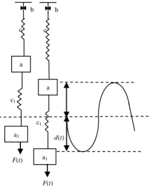
u
(10)Physical system with two degree of freedom described by the mathematical model is shown in fig 1:
Fig. 1. Physical system with two degree of freedom
Using an analytical method for solving, for example the Laplace method [2] the vibration expression is obtained the according to the time function:
0025 , 0
0036 , 0 ) 953855 , 2 sin( 0626 , 0
05296 , 0 ) 953855 , 2 cos(
128 , 1
973 , 0 ) 6597 , 0 sin( 5373 , 0
51957 , 0 ) 6597 , 0 cos(
467 , 0
4 , 0 sin 6 , 0 467 , 0 cos ) (
) ( ) (
267244 , 1
23169 , 0
2 1
t t
e
t t
e
t t
t u
t u t u
t t
, (11)
The test system with three degrees of freedom [2]
m
m
m
5
,
1
0
0
0
0
0
0
2
M
,
b
b
b
b
b
b
b
11
2
0
2
8
4
0
4
16
B
,
k
k
k
k
k
k
k
4
0
3
2
0
2
6
R
(12)(t)
F(t)
cos
0
0
1
(13)It is considered m = 1000 kg, b = 25 K·N·s/m și k = 1000 K·N/m.
The initial conditions are:
0
0
1
0
)
U
0u(
,
0
1
1
)
0
(
0.
V
u
. (14)II. THE PRESENTATION OF THE CALCULATION METHODS APPROXIMATELY TESTED
The calculation methods approximately tested are: β method of Newmark, method of the central differences, methods of approximating the solution by polynoms of the third degree, residual methods and approximation methods with sinusoidal functions.
A. β
Method of Newmark
method of Newmark [4] starts from the hypothesis that within the time investigated
[
t
i,
t
i1]
the F(t)d(t) a
b
c
a1
c1
a b
c
a1
c1
acceleration is constant and equal to the average of the accelerations at the ends of the range width.
]
[
2
1
)]
(
)
(
[
2
1
)
(
1.. ..
1 .. ..
..
u
t
iu
t
iu
iu
iu
(15)It is marked the range width with
h
t
i1
t
iRelation for accelerations becomes
)
(
2
)
(
.. 1 .. .. ..
i i
i
u
u
u
u
(16)Using the original conditions
(
u
(
t
i)
u
i,u
(
t
i)
u
i ..
) and integrating twice there are obtained the relations of recurrence which shall be modified by Newmark by inserting the coefficient
)
(
2
1.. .. .
1 .
i
i
ii
u
u
h
u
u
(17)1 .. 2 .. .
1
)
2
1
(
i
i
i
ii
u
h
u
h
u
h
u
u
(18)The standard form for the Newmark method is with = .
In the work [1, 6] it shows that: for method is stable no matter the chosen
time frame;
for , the method is stable only if the value of the report c = hn (Tn period of oscillation of the
way their own order n) meets certain conditions as follows
if = 0 must be that c would be c 0,318,
if = must be that c would be c 0.450, (19)
if = must be that c would be c 0,551.
The application of the Newmark method in the case of adequate attenuation systems, described by the equation
M
u
B
u
R
u
F(t)
, in the initial conditions u(0) = u0 ,u
(0) = u'0, consists in thedetermination of the response at time t1 (denoted by
U1) from the relationship
0 0 2
0 0 0 1 2
0 0
1 2 1 2
2 2
1
4 1 2
1 2
u B h v B β h
u R v B F M B β h I β h
v M h u M F h β U R h β B h M
n
(20)
The other components at the times t2,...,tn, shall be
determined successively from the equation
12 2
1 2 1 2
2 2
1 2
2 1 2
i i
i i +
i + i
U R h β B h M U R β) ( h M
F β F β) ( F β h U R h β B h M
(21)
For instance for t2 ( i=1) shall be calculated on the
basis of
u
i
u
1 (determined by the earlier relation),and depending on
u
i1
u
0 (known from the original conditions).Observation. Relationships are array type, which means that the determination of the solution
u
i1involves reversing the matrix
M
h
B
β
h
R
A
22
(22)B. The method of the central differences
The
method of central differences [6] considers the vector u(t) as a function of time for which it is written the development in Taylor series to the right and to the left of the point t = tiu(ti + h)= u(ti) + h
u
(ti) +u
(t
)
h
i
2
2+ ...., (23)
u(ti - h) = u(ti) - h
u
(ti) +u
(t
)
h
i
2
2
- .. (24)Disregarding the superior terms from the Taylor development we find that the method of the central differences is the method of Newmark for the
0
.For the time t1response determination(denoted by U1) is obtained from the relationship
0 0
2 0 0 0
1 2
0 0
1
2 2
4 2 1 2
u B h v B h u R v B F
M B h I +h v M h u M U B h
M
-n
(25)
For the other times t2,...,tn, the answer is determined
successively from the equation
1 2
2 1
2 2
2 i+ i i B M U
i-h U R) h M ( F h U B h
M
(26)
Observation. The method of the central differences as a particular case of method of Newmark for
0
, shows that it is necessary for maintaining stability, to have fulfilled the condition c = hn 0,318 [6]C. Method A3A4
Time field
t
[
0
,
b
]
can be broken down into mintervals of time
m
b
t
h
.The method proposes the approximation of the vector on the go with a polynomial degree of the third degree for any interval of time
[
t
i,
t
i1]
,
i
0
,...,
m
3 4 2 3 2 1
)
(
t
A
A
t
A
t
A
t
u
(27)Starting from the time interval
[
t
0,
t
0
h
]
we consider initial conditions0 .
0
,
(
0
)
)
0
(
u
u
v
u
(28)we provide that the resulting polynomial degree interpolation to verify that point. Get two of the constants of the model for the approximation, so that the resulting polynomial degree cannot be written in the form in
) ) ( 3 ) (( ) ( ) ( )
( 0 0 2
3 0 4 2 0 3 0 0
0 v t t A t t A t t t t t
u t
u
(29)
In order to determine the other two unknowns (
A
3,
A
4 ) we provide thatu
(
t
)
to verify the modelin the points
t
0
h
and2
0h
t
, which returns to thesystem of equations
) ( ) ( ) ( ) ( ) 2 ( ) 2 ( ) 2 ( ) 2 ( 0 0 0 . 0 .. 0 0 0 . 0 .. h t F h t u R h t u B h t u M h t F h t u R h t u B h t u M
(30)
We get the two equations with two unknowns
)
(
)
(
)
2
(
)
2
(
0 0 0 0 4 4 3 43 0 0 0 0 4 34 3 3h
v
u
R
Bv
h
t
F
A
a
A
a
h
v
u
R
Bv
h
t
F
A
a
A
a
(31)Where they knew each other
). 3 ( ) ( ) 2 ( 3 ) ( 6 , ) ( 2 2 ), 2 3 ( ) 2 ( ) 2 2 ( 2 3 ) 2 ( 6 , ) 2 ( 2 2 2 0 2 0 0 4 2 43 0 2 0 0 34 2 3 h t h R h t Bh h t M a h R Bh M a h t h R h t h B h t M a h R h B M a (32)
Using the constants
A
3,
A
4 shall be calculatedthe movement and speed at
t
t
0
h
, with the relations ) 34 ( ). 2 ( 3 2 ) ( ) 33 ( ), 3 ( ) ( 0 4 3 0 0 . 0 2 4 2 3 0 0 0 h t h A h A v h t u v h t h A h A h v u h t u u D. Method A3A4 the smallest squares
Method A3A4 cmmp is similar to the method A3A4 except for the fact that the method of the smallest squares to determine the constants of the
4 3
,
A
A
.The relations 27 -29 are valid in the case of this method.
The constants
A
3,
A
4 are determined by minimizing the objective functionmin
)
(
)
,
(
2 . 1 .. 4 3 2
k k k
m
k
k
B
u
R
u
F
u
M
A
A
F
(35)It is used a division of the range
[
t
0,
t
0
h
]
ofm
2 spaced points relative to one another with the2 1
m
h
h
, so that the points on which they arecalculated amount of relationship (35) are:
h
t
h
m
t
kh
t
t
h
t
t
0,
0
1,...,
k
0
1,...,
0
2 1
0
(36) The method of the smallest squares leads to a system of two equations with two unknowns from which are derived constantsA
3,
A
4 (valid for range)A
3,
A
4.For the calculation of the movement and speed are used relations (33),(34).
E. The iteratively - residual method
The time field
t
[
0
,
b
]
can be broken down into mequal time intervals or not.
For the presentation of the proposed method we
consider the equal time intervals
n
b
t
h
.The method proposes the approximation of the vector on the go with a polynomial degree of the third degree for any interval of time
[
t
i,
t
i1]
,
i
0
,...,
n
, seerelation (27).
Be imposed two conditions, namely polynom to verify the initial conditions (28) to
t
t
0 andh
t
t
t
t
0
0
.We give the values at the end of the range to
u
t
t
v
u
t
t
u
(
)
,
(
0
)
.0 (37)
Obtain a resulting polynomial degree interpolation [5]
u
t
t
v
u
t
t
u
(
)
,
(
0
)
.0 (38)
within which the interpolation expressions are:
;
t)
(
t
Δt
t
t
(t)
Φ
;
t
t
t
(
t
(t)
Φ
2 3 2 2 3 3 2 2 12
)
(
2
)
3
1
(39) . t) ( t Δt t (t) Φ ; t) ( t t) ( t (t) Φ 2 3 2 4 3 3 2 2 3 2 3 (40)within the framework of the iteratively residual method -with two other unknown namely with the movement
u
and speedv
.For the purpose of determining u, v method uses Galerkin conditions [3], which require that the residue to be orthogonal to the functions of the interpolation
t Δ
i t
Δ
i
(t)
ε
(t)
Φ
(t)
ε
(t)
Φ
0 4
0 3
0
0
(41)
where
i(
t
)
is the residue.Note1. Using the model of the system and the function of approximation , from the relation (38), we obtain the calculated value
u(t)
R
(t)
u
B
(t)
u
M
t
F
c(
)
.
The residue is the expression
F(t)
v
u
v
u
t
F
t
F
(t)
ε
i
c(
)
(
)
1
0
2
0
3
τ
4
τ
(42)The conditions (41) determine a linear system from which there are derived the two unknowns (travel
u
and speedv
).On the following interval of time
u
and
v
represents the initial conditions, this allows you to resume calculations.Note2. For integration there is not necessary to use an approximate method because the integrals contain some products of two algebraic functions
(t)
Φ
(t)
Φ
3,
4 are functions of the 3rd
degree and can be expressed by
3 2 2 1 2
1
,
,
)
(
t
t
t
(43)The second algebraic function is the
3 4 2 3 2 1 4 3 2
1
,
,
,
,
)
(
t
t
t
t
(44)The integral can be solved analytically, obtaining a polynomial degree
t t
t
dt
0
0
(45)
7 4 2 6 3 2 4 1 5 2 2 3 1 4 1 2 2 1 3 1
1 ( )
7 ) ( 6 ) ( 5 4
3 ( t) t t t
β α β α t) ( β
α
III. PRESENTATIONOFTHERESULTS
The solution shall be made on a interval 25 seconds, with a h=0.1s, which means that are displayed 250 points.
The relative standard deviation shall be determined by the relationship
100
analiticanalitic calculat
k
u
u
u
(46)and the average value of the irregularity shall be calculated with
nk
k
med
abs
n
1)
(
1
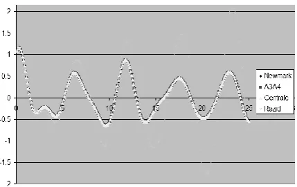
(47)The test system with two degrees of freedom
In figure 2 there are shown the results for the system with two degrees of freedom. The analytical solution (11) is called "Analytical".
Fig. 2 Moving the system 1 according to the time
In figure 3 there are shown the percentage deviations of the value of the points approximated reported to the value determined analytically - with the equation (11), only for the methods A3A4 and A3A4cmmp
It is found that the irregularities of the two methods there are different when they pass through the zero of the analytical solution.
For the purpose of decreasing the irregularity has been used a weighted average mediation, giving a degree of trust more than the solution as determined by means of the A3A4 method, so that the curve called "Media A3A4" is calculated with the
3 / ) 4 3 4
3 * 2 ( 4
3A A A CmmpA A
MediaA (48)
In table 1 there are presented the average deviations in percentage for the 250 points.
TABLE 1
Method
The average deviation
Deviation at t=4s
Deviation at t=7.4s
Deviation at t=19.7s
Newmark 6.66 3.9 6.59 0.58
Central dif. 6.13 3.7 5.86 0.35
Reziduu 18.78 2.98 0.43 13.03
A3A4 6.11 3.73 5.81 0.23
A3A4cmmp 12.45 4.76 8.35 2.03
Med A3A4 2.81 0.9 1.09 0.82
In columns 3 to 5 there are presented the irregularities at the three values of the time where values are obtained large (usually at the passing through the zero of the analytical solution). It is found that the Newmark methods, differences in central and A3A4 lead to deviations comparable average at around 6 %.
The technique of averaging the weighted average of the results of the A3A4 and A3A4cmmp determines both decrease (twice) droop as environments and reducing the significant deviation when they pass through the zero of the solution.
The test system with three degrees of freedom
Figure 4 shows the calculation results for the test system with 3 degrees of freedom.
It is found that 3 of the methods lead to comparable results, and the residuum method lead to oscillations are maintained.
It can be concluded that the residue method cannot be applied in the case of systems with more than 2 degrees of freedom.
Calculating the relative deviations of a method of each other get Newmark-Diferencentral you 8%, Newmark-A3A4 11.73%, central differences-A3A4 3.97%. We can reach the conclusion that the method of the central differences and the method A3A4 lead to results (within the limit of 4%).
IV. CONCLUSIONS
Using the test with two and three degrees of investigations have been obtained comparable results for the Newmark methods, central differences and a new method of A3A4 proposed in the framework of the work.
The method of design of the residue on the functions of the interpolation (Galerkin) leads to large deviations in the case of the test with two degrees of freedom (17.78%) and does not lead to a fair solution to the test with three degrees of freedom.
REFERENCES
[1]Connor J.J., Brebia C.A., The finite Element Technique, Santhamton, 1976;
[2]Dinu O. A system of automatic acquisition of data in real time for monitoring the vibration, UNITG.- PhD paper, manuscript, 2015;
[3]Dorn W.S., Mc Cracken D.D., Numerical Methods with programs in FORTRAN IV, „Tehnica” Publisher House, Bucureşti, 1976.
[4]Newmark, N. M., A method of computation for structural dynamics, Journal of Engineering Mechanics, ASCE, 85 (EM3) 67-94, 1959.
[5]Posea N., The dynamic calculation of the structures, “Tehnica” Publishing House, Bucharest, 1981;
[6]Warburton G. B., The Dynamical behavior of structures, Pergamum Press, London, 2014;