Volume 08 Issue 06 (2019) Nov.-Dec 2019

International Journal of Advances in Management and Economics

Available online at:

www.managementjournal.info

RESEARCH ARTICLE

Mathematical Risk Modeling: An Application in Three Cases of

Insurance Contracts

Ramzi Drissi

College of Islamic Economics and Finance, Umm Al-Qura University, (Saudi Arabia) and University of Carthage, (Tunisia).

Abstract: Risk is often defined as the degree of uncertainty regarding the future. This general

definition of risk can be extended to define different types of risks according to the source of the underlying uncertainty. In this context, the objective of this paper is to mathematically model risks in insurance. The choice of methods and techniques that allow the construction of the model significantly influence the responses obtained. We approach these different issues by modeling risks in three base cases: basic insurance of goods, life insurance, and financial risk insurance. Our findings show that risk modeling allowed us to better measure certain events, but did not allow us to predict them accurately due to a lack of information. Therefore, good modeling of the risk determinants makes it possible to modify the probability associated with the occurrence of a risk. While it cannot predict exactly when a risk will occur, it can help make decisions that will reduce its effects.

Keywords: Basic insurance, Life insurance, Mathematical models, Financial risk, Biometric function.

Article Received: 30 Sept. 2019 Revised: 10 Oct. 2019 Accepted: 22 Oct 2019

Introduction

One of the major areas of research in recent years has been modeling and estimating risks, in which the latter exhibits several sources of uncertainty[1]. Risk and opportunity play an important role in the insurance industry: If there were no risk, there would certainly be no insurers. The object of any insurance contract is risk; at the same time, risk is a specific element of insurance. Risk comprises danger, jeopardising goods, and insurance companies can protect businesses from which goods and businesses [2].

In its classical and practical form, insurance represents financial protection from losses caused by the occurrence of insured risk. Insurance represents a willing agreement based on an insurance contract that is concluded between the insurance company acting as the insurer and the insured person (natural or legal). The insurer offers the insured protection for the risks it assumes and accepts liability for compensating the insured party for damages supported in exchange for payment of an insurance policy paid in advance [3].

Risk protection may be regarded as a specific commodity or service that is bought or sold

on the financial services market. To be insurable, risk must comply with certain criteria which can be classed into risk and opportunity, both referring to future and uncertain events [4]. In the insurance business, risk is considered to be an undesired event, not only from the viewpoint of the client but also that of the insurer. Only those events that can result in a material loss can be insured. Otherwise, risks can be classed according to the following:

 Insurability: pure and speculative risks

 Implications and their nature: fundamental and specific risks

 Management: static and dynamic risks

 Effect on insurability: insurable and non-insurable risks

business. Insurance policies can only cover those events that result in a loss. To be insurable, a risk has to fulfil certain criteria[6], such as the following:

 It must be calculable; that is, it has to be calculable in terms of a probability ranking between 0 and 1.

 It must be unavoidable.

 It must be impossible to be aware of risk.

 It must be financially supportable in terms of magnitude and frequency by the insurer.

 It must be compensatory; that is, the insured party must compensate its financial loss resulting from the occurrence of the insured risk.

 It must be contractual, namely, it must carry over the protection provided for in the insurance contract.

Risk modeling allows us to better measure the occurrence of certain events, but it does not allow us to predict them accurately [7-8-9]. The objective of this paper is to mathematically model risks in three base cases (basic insurance of goods, life insurance and financial risk insurance), illustrating how the choice of methods and techniques that allow the construction of the model significantly influence the responses obtained. We approach these different models through some examples.

Our findings demonstrate that risk modeling allows us to better measure certain events, but does not allow us to predict them accurately due to a lack of information. Indeed, it is impossible to predict the future, and modeling is not accurate. The latter teaches us to cope with uncertainties; to accomplish this, it is possible to tame the chance, define it and control its effects.

The remainder of the paper is structured as follows: First, Section 2 lays out the mathematical modeling of basic insurance for goods with systems used to calculate the value of the damage compensation. Then, Section 3 presents the mathematical model of risk in life insurance using biometric functions, all of which are illustrated with simple examples.

Following this, Section 4 clarifies the mathematical modeling of risk in the insurance business. Finally, Section 5 concludes the paper.

Mathematical Modeling of the Basic Insurance of Goods

The object of a contract consists of the goods mentioned in the contract by either specifying a real individual value for each good or indicating a group of goods, such as complex insurance covering an entire household. The insured person has the obligation to maintain the asset during the execution of the insurance contract.

If the insured person does not fulfil this obligation, the insurer has the right to terminate the insurance contract and re-instate the contract when the insured remedies the situation [4]. The liability of the insurer starts 24 hours after the day when the insurance policy was paid and stops on the last day of the contract duration. Should the insured event happen, there are three systems used to calculate the value of the damage compensation:

 Proportional coverage system allowing the calculation of compensatory payment using the following formula:

(1)

Where, represents the compensatory payment, the Domage, the Insured amount, and the real value of the asset on the moment of risk occurrence.

 The system of the first risk calculating compensatory payment according to the formula:

D

  

P

D

Sa

The compensatory payment covers the damage not exceeding the insured amount. Otherwise, the occurrence of the insured risk may generate either a total or a partial loss. If the loss is total, therefore, the Domage (P) is equal to the real value of the asset on the moment of risk occurrence (Vr), and according to the proportional coverage principle:

Sa

D

Vr

Sa

P

D









According to the principle of first risk

Sa

D

P

For the application of this model in practice, we can identify three Situations:



Vr



Sa



D



P



Sa

 Vr SaDP;DSa



Vr



Sa



D



P

According to the partial coverage principle (Limited liability):

Vr

Sa

P

D





We can identify two situations:



Sa



Vr



D



P

 ii.

Sa



Vr



D



P

According to the principle of first risk

Sa

D

P

D







We can identify three situations:



Sa



Vr

 

D

P if D



Sa

 D  Sa if P  Sa  D = Sa if P > Sa

 The system of limited liability allows including a clause in the contract whereby the insured remains his own insurer for a franchise, that is a determined amount that is not to be compensated by the insurer, amount that can be of two kinds:

 Deductible franchise to be deduced from the damage value whatever the size of the damage, a system that allows motivating the insured to prevent the occurrence of risk. The compensation payment is calculated according to the formula

Sa

D

F

P

D









wherein F = franchise.  non-deductible franchise (depreciated or

simple) to be calculated according to the formula:

D



P



D



Sa

if P > F, D = O if

F

P



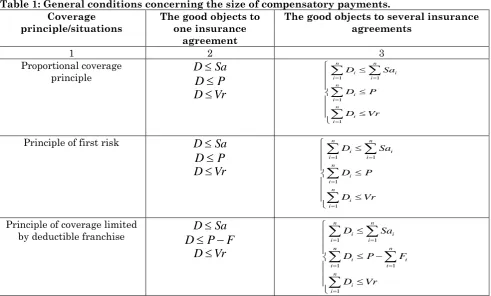
The Table below contains the general conditions concerning the size of compensatory payments upon the occurrence of the insured risk. The table provides information for the case of a good/asset insured by one or several insurer/s, using the three principles to cover the damage.

Table 1: General conditions concerning the size of compensatory payments. Coverage

principle/situations The good objects to one insurance

agreement

The good objects to several insurance agreements

1 2 3

Proportional coverage

principle

D

_D



_

Sa

_P

Vr

D



1 1

1

1

n n

i i

i i

n i i

n i i

D Sa

D P

D Vr

 





 _

 

 _

  

 



 

 

Principle of first risk

_D

_

_Sa

P

D



Vr

D



1 1

1

1

n n i i i i

n i i

n i i

D Sa

D P

D Vr

 





 _

 

 _

  

 











Principle of coverage limited

by deductible franchise

_D

D

_



_P

Sa

_

_F

Vr

D



1 1

1 1

1

n n i i i i

n n

i i

i i

n i i

D Sa

D P F

D Vr

 

 



 _

 

 _{ }

  

 













Where represents the compensatory payments value, the Damage suffered, the Insured amount, and the real value of the good upon occurrence of the insured risk, (F) the franchise, and (I) the number of insurance agreements.

There are Two Working Alternatives The First Alternative has Three Stages Calculation of the damage for each

insurance agreement

of compensatory payment (column 3 of the table above)

 Application of the adjustment procedure in order to comply with condition 2.

Condition 1o

1 1

n n

i i

i i

D

Sa

 







is always observed as it is observed by each individual insurance agreement.

Condition 2 o

1

(

)

n i i

D

P







, respectively

1 1

(

)

n n

i i

i i

D

P

F

 

 





may or may not be observed, which is why the re-adjustment procedure is needed in order to observe the principle of proportional coverage. If condition 2 is observed, so the

condition 3 o_:

1 1

(

)

n n

i

i i

D

Vr

 







as the damage to the asset cannot exceed the value of the asset itself upon occurrence of the insured risk.

The re-adjustment procedure for the proportional coverage principle calls in the formula:

*

1 i i n

i i

P

D

D

Sa







(2)

Where in * i

D is a compensation to be paid

and D_i is compensation calculated for each

contract.

Re-adjustment according to the limited liability principle, deductible franchise, shall be calculated according to the formula:

*

1 n

i i i n

i i

P F

D D

Sa 



 





(3)

The Second Working Alternative Comprises two Stages

 Establishing the part of the damage that is to be covered by each insurer

 Establishing the compensation due by each insurer according to the coverage system adopted.

The Possible situations for each type of damage to be covered by each insurer are given in the following Table:

Table 2: Situations of damage to be covered by the insurer Situations

Damage



_Sai

_

_Vr

i

Sa



Vr





Sa

i



Vr

Total damage (P = Vr)

i i

i

Sa

P

P

Sa

 



i i

i

Sa

P

P

Sa

 



i i

Sa

P

P

Vr

 

Partial damage (P < Vr)

i i

i

Sa

P

P

Sa

 



i i

Sa

Pi

P

Sa

 



i i

Sa

P

P

P

 

i i

Sa

P

P

Vr

 

Wherein

P

_i is the damage to be covered by insurers.

Mathematical Model of Risk in Life Insurance Using Biometric Functions

Biometrical functions1 _{[10-11] are}

mathematical relations between average biologic coordinates of individuals making up a certain population and financial indicators used in calculating life insurances.

1 _{Other biometric functions relate to disability, mortality of}

The Biometrical Functions Include[12]  Survival function noted hereafter with

l

_x

representing the average number of persons from a homogenous population alive at the age of x years. If we note with



 Life or survival probability: we will note it withp x y



,



. It represents the probability

for a person aged x to be still alive when

he/she is y years old.

A discrete case probability is calculated as the relationship between the number of favorable cases and the number of possible cases:

cases possible

of Number

cases favorable

of number p

_ _

_

_ _

_

 (4)

The life probability notations will be:



l

_x for the number of possible cases i.e. all

the persons alive aged n years old that

will still be alive at the age of y;

 l_y for the number of favorable cases

Making the replacements in formula (4), the

result is

( , )

y

x

l

p x y

l



If we consider that

y

 

x n

, wherein n is

the number of years after which the probability of survival is calculated, then we can make the replacements in the formula

( , )

y

x

l

p x y

l



and the result is defined by the

following expression:

( , ) x n x

l p x x n

l 

  (5)

In formula 5, we will replace

p x x n

( ,



)

with



n p x



, i.e. the probability for a person

aged x to be still alive after n a year or at

the age of



xn



years. The result is getting

the following formula:

x n x

l

n

p x

l



  

(6)

Represent the death or decease probability. We will note

q x y

( , )

for the probability that

person-aged x years be dead at the age of y

years. At the age of y a person may be

either dead or alive, so one of the following cases will take place:

( , )

( , ) 1

p x y



q x y



(4)

Which allows the calculation of the probability of death:

(x y, ) 1 (x y, )

q   p and replacing _{( , )}

x y

y x

p

l

l



.

The result will be:

,

(x y)

1

y x

l

q

 

l

(5)

If we express y as a function ofx, i.e.

y



x



n

in the formula _{( , )x y} y

x

l

q

l



the

result will be

,

(x y n) 1 x n

x

l l

q _    (6)

and noting



n q x 



for q_{(x y n,  )} we have:





1 x n

x

n q

l

x l

    (7)

The relationship between life and death probability can be expressed as follows:



n p x



+



n q x 



=1 (8) Death Probability Between two Ages

We will note

m

q x

n



_{ }











for the probability

that a person aged x decease between the ages x + m and x + n

x x+m x+n

The person lives the person dies

The person must live (x + m) years, which is quantified by the survival probability p_{(x x n,  )}.

Once the person is



xm



years old, we need

to calculate the probability for that person to be dead by the age of



xn



years. The

probability is a function of

q

_{(x m x n ,  )}.

Thus:

,

(_{x x m}) (x x m, )

p

x

n

q

m

q

 

Replacing the probabilities p_{(x x m,  )} and q_{(x x m,  )} with survival, functions

(x x m, ) x m

x

x

l

l







and

( , )

1

x x n

m x

n x

l

q

l

 







the result will be:

(1 ) ( ) ( )

x m x n x m x m x n x m x n

x x m x x m x

x m x n x

l l l l l l l

m q x

n l l l l l

l l

m q x

n l

      

 

 

 

     

    

(9)

Let's start with a simple example. We will illustrate the calculation system through the example of a person aged 40. Knowing that the survival probability for an individual

aged after 10 and respectively 15 years is 0,9581 and 0,9199, we will calculate the probability for the person to die between the ages of 50 and 55.

40 years 50 55 years

The person lives the person dies

Applying the formula 40 10 40 15 50 55 40

40 40

10 10

15 15

x m x n

l l l l l l

m

q x q

n lx l l

      

      

40 55

40 50 40

15

10

l

l

l

l

q





but ₀ 50 4

1

0 0

4 l

P  and 55 0 40

4

15 l

l P 

The result is that

40

10

0

.

9581

0

.

9581

0

.

9199

0

.

0982

40

10

40











p

q

%

82

,

3

0382

.

0

15

10

40





q

The probability for the insured risk to occur is 3.82%.

Mathematical Calculation of Average Risk

S(t) as the amounts paid by the insurer until

the moment “t” and the policies paid by the insured until the same moment, as assessed at the beginning of the insurance Anand [13]. If at the moment “t” the D > 0 the insurer

will register a loss if D < 0 the insurer will gain. During the contract, duration there has to be a balance of the financial operation of insurance [3]. This balance can be expressed by the formula defined as follows:

0 0 0

1

* * ( ) ( ) * * ( ) 0

l t

lx

t e u du e P u du dt

lx

  

  

_{   }  _

 _   _ 

 

 _{  }







(10)

Showing that the average value of the difference between the paid policies and paid compensations is equal to zero. For a vast number of insurances, the average value of the amounts paid to the insurer coincides with the value paid by the insurer as compensation. Insurances may be regarded as a game that ends up in gain or loss for the

insurer or the insured. For the insurer, insurance is a game with a large number of rounds, equal to the number of clients. Some of the rounds end up in victory, others in loss. The insurer must always look for new clients for the most innovative forms of insurance in order to ensure a fair average benefit. Under the basis insurance equation, it is given by the following expression:

0

0 0 0

( )

( )

t

n n n

t

lx t

lx t

lx n

e

t dt

e

e

P t dt

lx

lx

lx



 





 









_



_

_

_

_{ }

_









Average risk is calculated with the formula as follows:























 

)

(

))

(

)

(

(

0







  

Rx

e

du

u

u

P

e

lx

lx

Rm

u

(12)

Where in  is the insurance duration, Rx( )



is the mathematical reserve at the critical moment . and e-t _{is the amount paid by the}

insurer at the moment t updated at the beginning of insurance (t=0). The average mathematical risk corresponding to a yearly immediate rent is given by the formula:

Dx

Nx

a

Rm



_x(p)









1

(13)

We will illustrate all of the above through a simple example. Consider a person aged 40, concluding life insurance that supposes, in exchange for one payment, that the person will receive, at the end of every year, 120.000 u.m. if he is alive all assessment calculations

shall be made with the 5% yearly percentage and mortality information available for Tunisia.

What we need to calculate is the mathematical risk of insurance.

According to the formula

Dx

Nx

a

_xp









1

wherein x = 40,

hence

15724

.

9

/

12053

1

.

3046464

40

28 41

40 0

41









 

D

N

D

N

Rm

wherein  represents the critical

duration of the insurance and is the information we needed, thus p p x a

a  _ , a₄₀p a_p and

for p =5%, we have the double inequality ( ) 29 ) ( 40 ) ( 40

p p p

a a

a   . Since  is the smallest whole

number that satisfies the equation (p) (p) x a

a  _ the solution is  = 28

According to Formula (13)

Dx

Nx

a

Rm



_x(p)









1

This concerns the average risk per invested monetary unit.

For the entire amount S, average risk is calculated with the formula

Rm (S) = R,(1)S= 1.3046461 120000=156563.53 u.m.

The value of 156563.53 um of the average risk means that the critical duration of the insurance is  =28 years and in order to

achieve his objective the insurer party shall pay a one-off policy

JI(S) = a₄₀(p)S

But, a₄₀(P) 15.084709JI(S)15.084791200001810174.8u.m.

If the insured person lives 28 years, receiving at the end of each year an amount of 120000 u.m.

he will receive a total amount of ( ) ( ) 28

28 28

1 (1, 05)

120000 120000 1787777.5 . .

0.05

p p

A a u m





    

If the insured lives 29 years, at the end of each year he will receive an amount equal to

. . 04 . 1816931 141092

. 15 120000 05

. 0

) 05 , 1 ( 1 120000

29 )

(

29 um

A p      



If the insured lives less than 28 years, the insurer has a benefit worth and (C) as benefit.

084709

.

15

053

.

12

816

.

181

40 41 )

(

40







28

( )

(1 1, 05)

1810174.8 120000 14.8981

0, 05

1810174.8 1787772

–

22402.8 . .

insurer

C

JI S

I

u

a

m



















The benefit of the insurer is 22402,8 u.m. If the person lives more than 28 years e.g. 29, the benefit of the insured will be:

28

(1 1, 05)

120000 1810174,8

0, 05

(120000 15,141092) 1810174,8

1816931, 04 1810174,8 6756240

insured

um C





 

  

  



As we have seen from the previous examples, risk modeling can not be done without quantifying some parameters. That's why part of the research is devoted to estimation.

In what follows, I will talk about the particularities associated with the estimate in the presence of a risk of default [8-14].

Mathematical Modeling of Risk in the Insurance Business

Financial risk is potential damage that the creditor might suffer[3]. The creditor may be a bank or a supplier and the risk would be related to the impossibility of the debtor to pay back [8].

The Following Risks may Occur in the Execution of Financial Transactions[3]  The commercial risk may occur in domestic

and foreign transactions due to the depreciation of the financial capability of the purchaser that is unable to pay back in due time to the seller;

 Risks generated by force majeure or natural calamity situations that render the buyer unable to pay the amounts due to the supplier;

 Political risks generated by political phenomena and events, independent of the will and solvency of the buyer that render the buyer unable to pay the amount due to the supplier[14].

 Currency exchange rate risk, which consists of an alteration of the exchange rate between the currency of the exporter and that of the importer in the interval between the transaction conclusion and the moment of actual payment.

 Loan insurance represents a modality of insuring the financial risks [3-15] in order to protect banks for the amounts lent to the clients and to protect trading companies and manufacturers against the financial damage resulting from buyer insolvency.

According to the Location of the Exchange, Loan Insurance May be Classed in

 Domestic loan insurance

 Foreign loans insurance carried out through Exim bank

 Collateral insurance or bail represents the solidarity between the insurer and the insured in guaranteeing the creditor that the contractual liabilities of the insured party will be fulfilled.

 Fidelity insurance provides the insured party protection against damages generated by the trust towards employed personnel that manages the assets of the insured party.

Technical Elements of Financial Risk Insurance

 Amount insured for domestic loans

 Insurance policy for international loans

 Domestic loans insurance compensation Loan insurance is meant to protect the creditor (the insured party) against the financial loss generated by client inability to repay the loan [3]. The insured party may be a legal person that has the core activity of granting loans or delivering goods in exchange for multiple scheduled payments or asset leasing.

The Following Risks are Excluded from Insurance

 Risks generated by the force majeure under the contract between insured party and its clients

 Loss of profit due to the halt inactivity as a consequence of insured risk occurrence;

 Penalties due by debtor to the insured party for late payments;

 Losses due to change in the currency exchange rate and local depreciation;

 Fraud, mismanagement, bad faith management;

 bank inability to pay or bank bankruptcy;

 Political risks.

According to the Particularities of the Insurance Policy, the Following Types of Contract Exist

 Type A: transaction policy. The insurance is concluded for only one type of transaction, on a certain date with one or more clients;

 Type B: ongoing transactions policy that is concluded for an unlimited number of transactions concluded by the insured party, with one or more clients;

 Type C: turnover policy covering insurance for all businesses involving credit carried out by the insured party during a determined 12 months interval.

The Amounts for Each Type of Policy Shall be Established as Follows

 For type A policies the insured amount Sa

represents the total value of net outstanding debts of clients towards supplier at the moment of loan conclusion

(

Sa





Dr

)

.

 For type B policies the amount insured is the total value of net debt and represents a ceiling that the policy can not exceed during the entire contract duration.

 For type C policy the amount insured is established on the basis of estimative turnover assessed on the basis of current turnover. The insured party will pay a minimum policy and a deposit policy calculated as a percentage of the turnover, estimated for the contract duration. At the end of the insurance contract, the insured amount shall be recalculated according to

the actual performance, and the insurer will pay the balance.

The Maximum limit of the insurer liability represents the ceiling of the loan and (principal and interest). Otherwise, franchise represents a percentage of the insured amount that will apply for every client of the insured party.

Credit insurance can be concluded with a franchise upon demand from the client. Insurance policy will be determined on a yearly basis, applying a percentage according to the policy price for a given amount insured. The insurance will be effective upon loan conclusion or upon delivery of the first tranche of goods and expires upon the last payment of the granted loan, i.e. upon complete reimbursement of the loan[16].

Conclusion

The theory of insurance represents a very important and interesting field for exploration and research because the world’s insurance companies have become important participants in the economy. In this paper, we tried to give some basic notions about risk modeling, the choice of methods and techniques that allow us to significantly influence the answers obtained. We have approached these different models through some examples.

Our findings show that risk modeling allows us to better measure certain events, but it does not allow us to predict them accurately due to a lack of information. Indeed, it is impossible to predict the future and modeling is not accurate. This latter teaches us to cope with uncertainties. For that, it is possible to tame the chance, to define it and to control its effects.

The good modeling of risk determinants makes it possible to modify the probability associated with the occurrence of a disaster. Although it cannot accurately predict when it will occur, it can help make decisions that will reduce the effects.

determinants makes it possible to modify the probability associated with the occurrence of a risk. Although it cannot predict exactly when it will happen, it can help make decisions that will reduce the effects. In addition, it is necessary to remember that the key to the success of modeling also lies in access to good information.

Insurance companies need to develop an information database as well as technologies for decision-makers. Modeling, if it is to be accurate, must work with enough data. Due to the lower costs of archives and database creation, this will not be a problem in the future.

References

1. Jaeger CC (2001) Risk, Uncertainty and Rational Action, Earthscan Risk in Society, 1st Edition

.

2. Fabozzi fj, Focardi SM (2004) The Mathematics of Financial Modeling and Investment management. New Persey: Wiley. ISBN 0-471- 46599-2.

3. Tang Q, Yang Y (2019) Interplay of insurance and financial risks in a stochastic environment, Scandinavian Actuarial Journal,1-20.

4. Jaeger CC, Renn O, Rosa E, T Webler (2001) Risk, Uncertainty, and Rational Action. London: Earhscan Publications.

5. Feng R, Yi Bingji (2019) Quantitative modeling of risk management strategies: Stochastic reserving and hedging of variable annuity guaranteed benefits. Insurance: Mathematics and Economics, 85:60-73.

6. Pflug G (1997) How to measure risk? Festschrift for F. Ferschl. Berlin: Physica Verlag

.

7. Wüthrich MV, Merz M (2013) Financial Modeling, Actuarial Valuation and Solvency in Insurance. Springer Finance.

8. Crosbie P, Bohn J (2003) Modelling Default Risk. Moody’s KMV Company.

Available at

http://www.defaultrisk.com/_asp/rd_mode l_35.asp.

9. Kloppenberg EP, Mikosch T(1997) ''Modeling extremal events for insurance and finance'', Springer-Verlag, Berlin.

10. Olivieri A, Pitacco E (2015) Introduction to Insurance Mathematics. Technical and Financial Features of Risk Transfers.. Springer International Publishing, Second Edition.

11. Yang LG (1978) Estimation of a Biometric Function. The Annals of Statistics, 6 (1):112-116.

12. Makowski M (2005) Mathematical Modeling for Coping with Uncertainty and Risk. Systems and Human Science - For Safety, Security and Dependability.

13. Anand P (1993)Foundations of Rational Choice under Risk. Oxford: Oxford University Press.

14. Denault M, G Gauthier, J-G Simonato (2009) Estimation of Intensity Models for Default Risk, Journal of Futures Market, 29 (2):95-113.

15. Linnerooth-Bayer J, Amendola A (2003) Special edition on flood risks in Europe, Risk Analysis, 23:537-627,