Long-Term Evolution of Russia s Market Integration

Munich Personal RePEc Archive

Long-Term Evolution of Russia’s Market

Integration

Gluschenko, Konstantin

Institute of Economics and Industrial Engineering, Siberian Branch

of the Russian Academy of Sciences, Novosibirsk State University

5 May 2020

Online at

https://mpra.ub.uni-muenchen.de/100118/

Long-Term Evolution of Russia’s Market Integration

K.P. Gluschenko

a

Institute of Economics and Industrial Engineering, Siberian Branch of the Russian Academy of Sciences, Novosibirsk, Russia

b

Novosibirsk State University, Novosibirsk, Russia e-mail: glu@nsu.ru

Abstract—This article considers an aggregated market represented by a staples basket and analyzes changes in the

degree of spatial integration of this market during 1992 to 2019. In an integrated market, interaction of demand and supply in the national market, and not in a regional market, determines the regional price of a good. Based on this, the strength of dependence of regional prices on regional quantities demanded serves as a measure of the degree of market integration.

Introduction.

A market consisting of spatially dispersed segments – regional markets – is

deemed integrated if only “natural” barriers restrict freedom of inter-regional trade. It is the

spatial dispersion itself that creates such barriers, making necessary to incur costs of

transportation goods between regions. In such a fully integrated market the price of a tradable

good in two regions will differ by no more than shipping costs per unit of the good. A

mechanism that maintains spatial equilibrium is the goods arbitrage, i.e., purchasing a good in

regions where it is cheaper for selling where it is more expensive. Therefore, the regional price

of a good should not depend on regional demand, since arbitrage eliminates changes in the price

caused by increase or decrease in demand.

Obviously, the national market is fully integrated in no one country. Many “artificial”

barriers restrict freedom of arbitrage (though, a part of them can be called as such somewhat

conventionally). These are regional protectionism, regional price control, activity of organized

crime, imperfect local markets for labor and real estate (which cause inter-regional differences in

distribution costs), institutional factors (which narrow the choice of trade partners, e.g., because

of long-term contracts, long-standing partnership, reputation of potential partners), etc. This

poses a question of the degree of market integration: how close is a market to the ideal, full

integration?

This question attracted great interest (mainly, among foreign researchers) with respect to

Russia of the 1990s, when it transited from the centrally-planned economy to market economy.

With the use of data on prices for different goods in various spatial samples and time spans, they

inquired by means of diverse statistical methodologies whether integration of the Russian market

improved in the course of the transition and whether it existed [1–6]. When the transition process

has mostly completed and the Russian market became “ordinary,” foreign researchers have lost

interest to the issue of its integration; mainly Russian economists have come to deal with it. They

consider integration of markets for both final [7–10] and intermediate goods [11, 12]. The author

has studied Russia’s market integration in some time spans belonging to the transition and

further times [13, 14].

More than a quarter of century has passed ever since the Russian economy turned to the

market way of development. It makes it possible to look at integration of the Russian market

“from a bird’s-eye view” and see how it has been changing in the course of transition from

planned to market economy and then, and what impacts of different macroeconomic shocks on it

have been. That is what this article aims at.

Methodology of the analysis.

As it follows from the aforesaid, a dependence of price for a

good in some region on quantity demanded there evidences that the market deviates from full

integration. The “strength” of such a dependence can measure the degree of market integration:

the stronger the dependence, the weaker the integration. The analysis applies a model based on

this idea that has been put forward in [13]. In general terms, the model is as follows.

Let

P

be the price of a good in region

r

, and

M

be income per capita in

r

;

D

(

P

,

M

) is the

demand function, and

S

(

P

) is the supply function. From the equilibrium condition for the

regional market,

D

(

P

,

M

) =

S

(

P

), the price can be expressed in terms of income per capita as

P

=

a

M

. So the dependence of price on per capita income replaces the dependence on quantity

demanded (statistical data on which are lacking). Assuming the demand functions to be the same

across all regions, we get for region

s

P

=

a

M

. Then

ln(

P

/

P

) – ln

T

=



ln(

M

/

M

),

(1)

where regions are arranged so that

P



P

;

T

= (1 +



);



is relative costs needed to carry

unit of the good between

r

and

s

. Let us use a widely adopted assumption that shipping costs are

determined by distance between regions,

L

: ln

T

=



+



ln

L

, where



is a coefficient

depending on unit of distance.

Inserting this relationship into Equation (1) and adding random shocks



, the following

econometric model is arrived at:

ln(

P

/

P

) =



+



ln(

M

/

M

) +



ln

L

+



.

(2)

Here,



is the elasticity of price differential with respect to income differential (as it is

proved in [13],



should be non-negative). It is its value (which essentially characterizes market

segmentation) that measures the degree of integration: the lesser the



, the stronger the market

integration. In a fully integrated market,



= 0. The observations are region pairs (

r

,

s

); their total

number equals

N



(

N

–1)/2, where

N

stands for the number of regions in a sample. Sequentially

estimating Regression (2) for every point in time, we get the dynamics of integration,



, during

Data.

The time span to be dealt with is 1992 to 2019. The econometric analysis is

performed with the use of annual and monthly data.

Integration of markets for individual goods does not provide a general pattern, as it can

significantly depend on particular features of one or another market. Therefore, it is desirable to

consider an aggregated market represented by a goods basket. For the sake of comparability, the

basket should be uniform across regions and time-invariant. There are a few indicators of the

costs of different baskets in the Russian statistics. These are the goods price index (a subindex of

consumer price index, CPI), cost-of-living index, the cost of the fixed basket of goods and

services, and the cost of the minimum food basket (staples basket). However, the baskets used to

compute CPI are not comparable across regions. While the goods coverage in regional baskets is

the same, the weights of the goods are region-specific (and change every year). The next two

indicators have started to be published only since the 2000s, so not covering the whole time span

of interest (moreover, the relevant baskets include, in addition to tradable goods, services).

Therefore, there is nothing to do other than consider the aggregated market represented by

the staples basket. This basket is uniform across regions; however, its composition has changed a

few times. It contained 19 foods in 1992–1996, 25 foods in January 1997 to June 2000 [15, p.

428], and 33 foods since July 2000 to present [16, Appendix 3]. That is why the analysis is

forced to deal with data on costs of unlike baskets and somewhat different region coverage for

1992–2000 and 2001–2019. The annual basket costs are computed as the averages of monthly

costs (for 1992, over 11 months), based on the fact that the Russian statistical agency computes

annual income per capita in the similar way.

The estimations for 1992–2000 (and the monthly estimations for February 1992 to June

2000) use the cost of the 25-food basket (hereafter, “basket-25”). The Russian statistical agency

has provided these data on author’s request (and it has specially computed the costs for February

1992 to December 1996).

_{The estimations for 2001–2019 (and the monthly estimations for July}

2000 to December 2018) use the cost of the 33-food basket (hereafter, “basket-33”) [17].

Therefore, the results obtained for these two time spans are not fully comparable. The

differences are not only in the compositions of the baskets and quantities of goods in the baskets

(see Table A1 in Appendix A). The cost of basket-25 relates to region’s capital city alone, while

the cost of basket-33 is the region average.

The monthly data on incomes per capita for 1992–2000 have been obtained directly from

the Russian statistical agency; these for 2001–2018 have been drawn from monthly bulletins

“Socio-Economic Situation of Russia.” The annual data for 1992–2012 have been drawn from

the Rosstat’s web-site;

_{the source of data for 2013–2019 is [18].}

The federal subjects of the Russian Federation are meant by regions in this article. A

federal subject that includes autonomous

okrug

(s) is treated as a single region. The sample used

for the 2001–2019 estimations covers 79 regions (3081 region pairs). It does not include the

Chechen Republic, Republic of Crimea, and the city of Sevastopol, as the data on them do not

cover the whole period. The sample for 1992–2000 does not include, in addition, the Republic of

Ingushetia, Jewish Autonomous Oblast, and Chukotka Autonomous Okrug because of

incomplete data. Besides, the price data are the same for the city of Moscow and Moscow

Oblast, as well as for the city of Saint-Petersburg and Leningrad Oblast, since the costs of the

basket is that in the capital city of region in that time. Therefore, these

oblasts

do not enter to the

sample as well. In total, this sample consists of 74 regions generating 2701 pairs.

In addition to the whole sample (Russia as a whole), the analysis deals with two

subsamples (see Fig. B1 in Appendix B). The first is Russia excluding difficult-to-access

regions. It differs from the whole sample in that it does not include remote regions, mostly, with

poor transport accessibility. They are regions that inherently cannot participate in arbitrage,

namely, the Murmansk, Sakhalin, and Magadan Oblasts, Kamchatka Krai, Republic of Sakha

(Yakutia), and Chukotka Autonomous Okrug. This subsample consists of 69 regions (2346 pairs)

in 1992–2000, and 73 regions (2628 pairs) in 2001–2019. The second subsample is European

Russia. In includes all regions from the European part of the country except for northern ones,

the Murmansk and Arkhangelsk Oblasts and Republic of Komi. It covers 51 regions (1275 pairs)

in 1992–2000, and 54 regions (1431 pairs) in 2001–2019.

The distances between regions are the shortest rail distances between their capitals [19, 20].

In the cases when railway communication is lacking, road, river, or sea distance is added. The

average distance from cities of the Moscow Oblast where the statistics observes prices according

to [21] to Moscow plus the distances to Moscow serve as the distances to this

oblast

, similarly

for the Leningrad Oblast.

Results.

Table 1 reports means and standard deviations of the dependent variable – price

differential

p

= ln(

P

/

P

) – and the explanatory variable – income differential

m

= ln(

M

/

M

) –

over all region pairs in a relevant spatial sample. They are denoted respectively as

p

,



(

p

) ,

m

,

and



(

m

) .

2 _{To date, the data have disappeared from the relevant web-page}

Table 1

. Descriptive statistics of variables

Russia as a whole Excluding difficult-to-access _regions European Russia

Year

p (p)

m

m

m

1992 0.207 0.163 0.227 0.392 0.179 0.141 0.150 0.336 0.170 0.136 0.068 0.268 1993 0.253 0.224 0.264 0.424 0.203 0.175 0.171 0.348 0.168 0.159 0.077 0.266 1994 0.274 0.259 0.326 0.450 0.200 0.159 0.233 0.382 0.147 0.117 0.172 0.331 1995 0.239 0.210 0.320 0.459 0.185 0.145 0.246 0.419 0.130 0.104 0.188 0.410 1996 0.225 0.221 0.277 0.498 0.162 0.132 0.201 0.464 0.104 0.089 0.152 0.456 1997 0.204 0.209 0.263 0.483 0.143 0.119 0.195 0.458 0.082 0.067 0.161 0.441 1998 0.191 0.193 0.281 0.491 0.132 0.106 0.214 0.468 0.102 0.086 0.186 0.458 1999 0.150 0.148 0.261 0.521 0.106 0.087 0.187 0.496 0.094 0.084 0.177 0.478 2000 0.157 0.159 0.265 0.517 0.110 0.092 0.200 0.499 0.088 0.078 0.203 0.477 2001 0.175 0.200 0.318 0.502 0.112 0.088 0.232 0.462 0.089 0.075 0.189 0.447 2002 0.164 0.197 0.314 0.489 0.103 0.083 0.224 0.442 0.083 0.075 0.177 0.435 2003 0.166 0.194 0.306 0.500 0.108 0.084 0.219 0.459 0.091 0.079 0.176 0.459 2004 0.189 0.214 0.310 0.479 0.125 0.097 0.234 0.446 0.095 0.075 0.196 0.448 2005 0.180 0.214 0.299 0.486 0.116 0.095 0.221 0.453 0.083 0.068 0.190 0.456 2006 0.192 0.223 0.289 0.458 0.125 0.098 0.216 0.427 0.093 0.073 0.191 0.428 2007 0.184 0.216 0.260 0.449 0.117 0.091 0.190 0.421 0.088 0.069 0.171 0.418 2008 0.173 0.188 0.236 0.388 0.115 0.086 0.171 0.357 0.091 0.067 0.156 0.351 2009 0.197 0.214 0.229 0.389 0.131 0.102 0.158 0.352 0.098 0.072 0.140 0.358 2010 0.183 0.199 0.199 0.380 0.122 0.097 0.127 0.341 0.091 0.068 0.114 0.348 2011 0.173 0.182 0.200 0.368 0.117 0.092 0.130 0.330 0.086 0.066 0.121 0.336 2012 0.204 0.203 0.182 0.370 0.145 0.112 0.113 0.331 0.105 0.079 0.107 0.334 2013 0.199 0.201 0.189 0.378 0.142 0.108 0.115 0.334 0.103 0.077 0.112 0.337 2014 0.192 0.193 0.180 0.361 0.135 0.104 0.106 0.313 0.100 0.076 0.113 0.309 2015 0.181 0.176 0.174 0.358 0.131 0.103 0.102 0.312 0.100 0.079 0.099 0.310 2016 0.196 0.194 0.185 0.368 0.140 0.107 0.109 0.320 0.111 0.087 0.109 0.317 2017 0.185 0.184 0.194 0.371 0.131 0.100 0.117 0.320 0.109 0.087 0.109 0.319 2018 0.187 0.188 0.206 0.383 0.132 0.100 0.124 0.326 0.110 0.087 0.111 0.329 2019 0.185 0.187 0.203 0.386 0.130 0.098 0.121 0.329 0.107 0.084 0.112 0.331

Since all

p

are nonnegative by construction, their mean and standard deviation can be

considered as aggregate indicators of price dispersion in the country or in one or another its part.

For instance,

p

is the logarithm of the geometric average of price differences,

P

/

P

. As ln(1 +

x

)



x

, the figures in the table can be roughly interpreted as represented in unit fractions, and not in

logarithms (

e

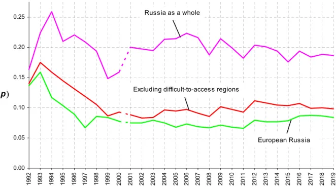
– 1 gives the exact values). Fig. C1 and C2 in appendix C show the evolution of

p

and



(

p

).

The price dispersion rose dramatically in the initial years of the market transformations. In

Russia as a whole, the average price difference reached maximum in 1994, equaling circa 32%

(=

e

– 1). After that, the price dispersion started nearly steadily decreasing and come to the

minimum in 1999–2000. In Russia as a whole, the average price difference decreased up to 16%

(=

e

– 1) in 1999. In 2001–2019, the price dispersion remained fairly stable, fluctuating within

a not wide range. Recall that the staples baskets used are different for 1992–2000 and 2001–2019

(that is why a line divides these time spans in Tables 1 and 2). As a result, jumps in prices in the

way from 2000 to 2001 reflect the change of basket (and, to some extent, region coverage), and

not a real phenomenon.

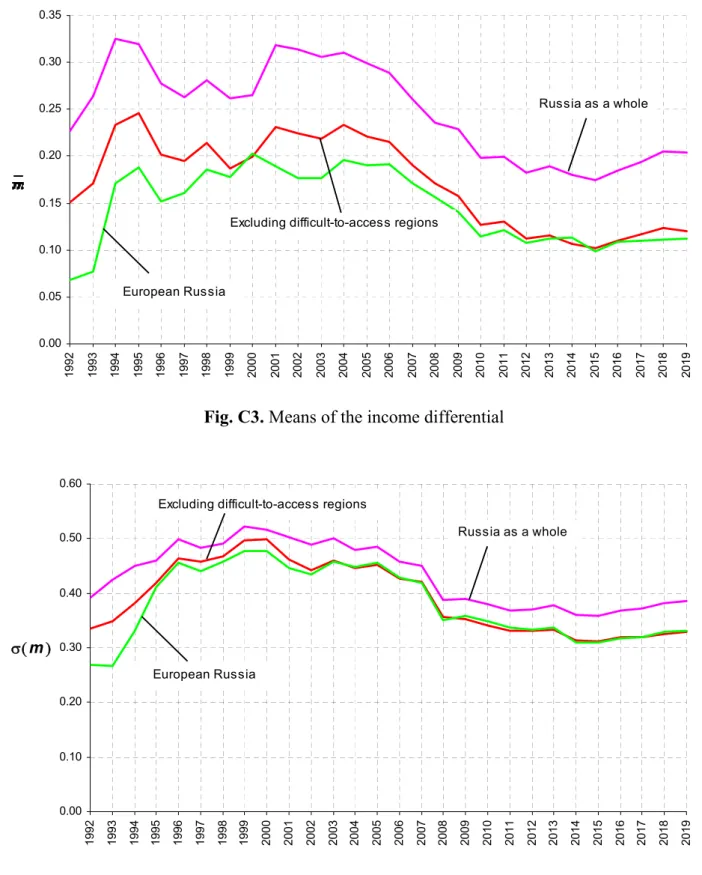
As for incomes per capita, their regional dispersion mainly increased up to 2004–2005.

After that, convergence of regions in incomes per capita started. It apparently stopped since

2015.

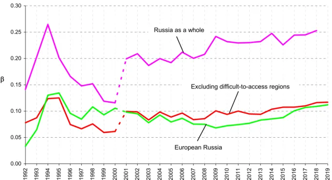
Table 2 reports results of the regression analysis with the use of annual data. Fig. 1 shows

the dynamics of Russia’s market integration characterized by changes in the values of



, the

degree of market segmentation.

Table 2

. Estimates of Regression (2) on annual data

Russia as a whole Excluding difficult-to-access _regions European Russia

Year

      p-value _{of }

1992 0.142 (0.008) 0.031 (0.003) 0.078 (0.008) 0.012 (0.003) 0.034 (0.013) 0.015 (0.005) 0.008 1993 0.203 (0.010) 0.077 (0.004) 0.087 (0.009) 0.050 (0.004) 0.065 (0.015) 0.010 (0.007) 0.136 1994 0.265 (0.009) 0.123 (0.004) 0.124 (0.007) 0.077 (0.004) 0.130 (0.009) 0.024 (0.004) 0.000 1995 0.201 (0.007) 0.110 (0.003) 0.125 (0.006) 0.073 (0.003) 0.135 (0.007) 0.013 (0.004) 0.000 1996 0.166 (0.008) 0.131 (0.004) 0.075 (0.005) 0.077 (0.003) 0.096 (0.005) 0.008 (0.003) 0.019 1997 0.148 (0.007) 0.137 (0.003) 0.066 (0.005) 0.079 (0.003) 0.085 (0.004) 0.008 (0.002) 0.001 1998 0.152 (0.007) 0.106 (0.003) 0.076 (0.005) 0.046 (0.002) 0.108 (0.005) 0.007 (0.003) 0.017 1999 0.119 (0.005) 0.065 (0.003) 0.059 (0.004) 0.018 (0.002) 0.093 (0.005) -0.006 (0.003) 0.059 2000 0.116 (0.005) 0.088 (0.003) 0.061 (0.004) 0.037 (0.002) 0.106 (0.004) -0.001 (0.003) 0.815 2001 0.199 (0.007) 0.088 (0.003) 0.099 (0.004) 0.027 (0.002) 0.098 (0.005) 0.003 (0.003) 0.216 2002 0.209 (0.008) 0.075 (0.003) 0.099 (0.004) 0.017 (0.002) 0.095 (0.006) 0.001 (0.003) 0.651 2003 0.187 (0.008) 0.076 (0.003) 0.083 (0.005) 0.018 (0.002) 0.078 (0.007) 0.003 (0.003) 0.292 2004 0.200 (0.008) 0.103 (0.003) 0.098 (0.004) 0.041 (0.002) 0.093 (0.005) 0.010 (0.003) 0.000 2005 0.192 (0.008) 0.106 (0.003) 0.089 (0.004) 0.042 (0.002) 0.079 (0.005) 0.008 (0.002) 0.001 2006 0.212 (0.009) 0.112 (0.004) 0.096 (0.004) 0.045 (0.002) 0.086 (0.005) 0.010 (0.003) 0.000 2007 0.200 (0.008) 0.109 (0.004) 0.084 (0.004) 0.040 (0.002) 0.075 (0.005) 0.014 (0.002) 0.000 2008 0.208 (0.008) 0.092 (0.003) 0.086 (0.004) 0.034 (0.002) 0.075 (0.005) 0.012 (0.002) 0.000 2009 0.242 (0.009) 0.107 (0.003) 0.101 (0.005) 0.045 (0.002) 0.068 (0.005) 0.016 (0.003) 0.000 2010 0.232 (0.009) 0.100 (0.003) 0.094 (0.005) 0.044 (0.002) 0.072 (0.005) 0.014 (0.002) 0.000 2011 0.229 (0.008) 0.089 (0.003) 0.100 (0.005) 0.040 (0.002) 0.074 (0.005) 0.013 (0.002) 0.000 2012 0.230 (0.009) 0.107 (0.003) 0.095 (0.006) 0.055 (0.002) 0.077 (0.007) 0.014 (0.003) 0.000 2013 0.232 (0.009) 0.104 (0.003) 0.094 (0.006) 0.054 (0.002) 0.083 (0.006) 0.014 (0.003) 0.000 2014 0.248 (0.009) 0.097 (0.003) 0.104 (0.006) 0.049 (0.002) 0.085 (0.007) 0.012 (0.003) 0.000 2015 0.226 (0.008) 0.084 (0.002) 0.108 (0.006) 0.044 (0.002) 0.088 (0.007) 0.012 (0.003) 0.000 2016 0.244 (0.009) 0.092 (0.003) 0.108 (0.006) 0.043 (0.002) 0.101 (0.007) 0.018 (0.003) 0.000 2017 0.245 (0.008) 0.076 (0.003) 0.110 (0.005) 0.032 (0.002) 0.107 (0.007) 0.018 (0.003) 0.000 2018 0.253 (0.009) 0.076 (0.003) 0.116 (0.005) 0.032 (0.002) 0.109 (0.007) 0.019 (0.003) 0.000 2019 0.250 (0.008) 0.078 (0.003) 0.117 (0.005) 0.035 (0.002) 0.112 (0.006) 0.019 (0.003) 0.000

Notes: standard errors of estimates are in parentheses; p-values of all estimates, except for  for European Russia,

0.00 0.05 0.10 0.15 0.20 0.25 0.30

1992 1993 1994 1995 1996 1997 1998 1999 2000 2001 2002 2003 2004 2005 2006 2007 2008 2009 2010 2011 2012 2013 2014 2015 2016 2017 2018 2019

Russia as a whole

Excluding difficult-to-access regions

European Russia



Fig. 1. Dynamics of Russia’s market integration by year

In the initial stage, 1992–1994, market segmentation increased dramatically. It is a stretch,

though, to speak about market of that time. (The estimates themselves for those years must

therefore be taken with caution.) Retail trade remained mainly state-run,

_{although it had been}

eligible for pricing on its own. The “money overhang” created by goods shortage in the previous

years made it possible a great increase of retail prices since January 1992. The “overhang”

disappeared quickly; then the “inflation spiral” started to act: in response to the rise in prices,

workers demanded wage raise, and increase in wages resulted in further rise in prices. These

processes were closed within regions, so creating strong inter-dependence between prices and

incomes in the region. Retail trade relied upon former sources of supply; inter-regional arbitrage

was out of the question as there were no owners interested in this (besides, information on prices

across regions was extremely scrappy).

Formation of genuine market – as a result of mass privatization and market

self-organization – can be attributed to 1994–1995. Since that time, integration of the regional

markets started improving. The 1998 crisis somewhat turned this process back (in a number of

regions, the exportation of goods was even prohibited). However, the crisis eventually became a

powerful force for further increasing integration. The collapse of the ruble exchange rate (from

5.96 RUR/$ as of January 1, 1998, to 20.65 RUR/$ as of December 31 [22]) forced the market to

switch from imported to domestic goods. A consequence was a substantial increase in

inter-regional trade and, accordingly, in integration of the Russian market.

3 _{It is worth noting that the official statistics recorded prices solely in state-run shops in that time. It added markets}

A strange feature can be observed in Fig. 1: in 1994–2000, the degree of integration in

European Russia is less than in Russia excluding difficult-to-access regions. Taking into account

much more developed transport infrastructure and lesser distances between regions in the

European part of the country than in the Asian part, one would expect the reverse pattern. The

reason will be discussed further.

Jumps while moving from 2000 to 2001 (they are shown by dashed lines in Fig. 1) are

caused by the change of staples basket used for the analysis. Available data on the costs of both

basket-25 and basket-33 for several months of 2000 allow comparing estimates obtained with

different baskets (and somewhat diverse region coverage) and understanding how great the

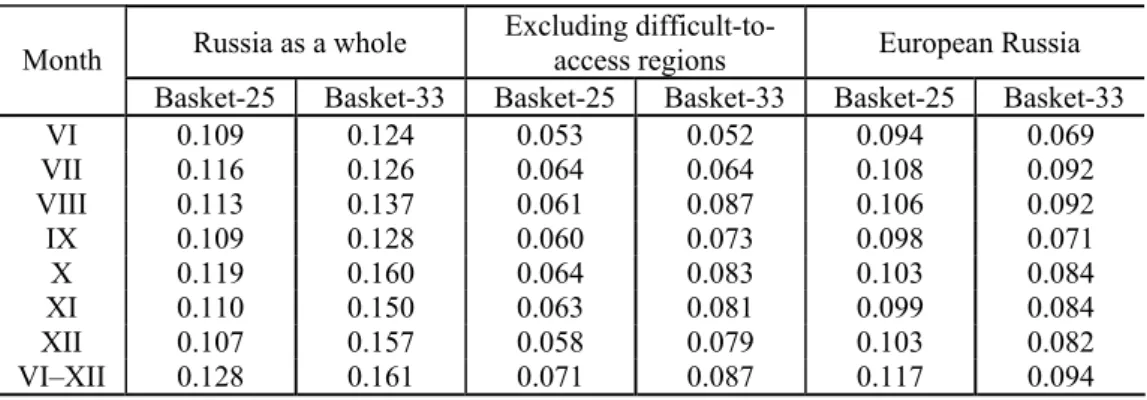
differences are. Table 3 tabulates these estimates by month and for June–December 2000 (with

data averaged over 7 months). Fig. D1 in Appendix В compares the estimates graphically.

Table 3.

Estimates of



on monthly data for June to December 2000

Russia as a whole Excluding difficult-to-_{access regions} European Russia

Month

Basket-25 Basket-33 Basket-25 Basket-33 Basket-25 Basket-33

VI 0.109 0.124 0.053 0.052 0.094 0.069

VII 0.116 0.126 0.064 0.064 0.108 0.092

VIII 0.113 0.137 0.061 0.087 0.106 0.092

IX 0.109 0.128 0.060 0.073 0.098 0.071

X 0.119 0.160 0.064 0.083 0.103 0.084

XI 0.110 0.150 0.063 0.081 0.099 0.084

XII 0.107 0.157 0.058 0.079 0.103 0.082

VI–XII 0.128 0.161 0.071 0.087 0.117 0.094

As Table 3 suggests, the discrepancies between respective estimates are fairly sizeable.

They are particularly great for Russia as a whole. The estimate of the segmentation degree over 7

months with basket-33 exceeds the estimate with basket-25 by 26%. The discrepancies for

Russia excluding difficult-to-access regions are somewhat smaller. In this case, the estimates

with basket-33 also suggest a higher degree of market segmentation, by 23% over

June-December. However, the degree of market segmentation of European Russia estimated with

basket-33 is less than that estimated with basket-25 (by 20% for estimates over 7 months).

A more detailed analysis evidences that there were no dramatic changes in Russia’s market

integration in 2001 as compared to 2000. Therefore, it can be believed (somewhat

conventionally) that the integration paths over 2001–2019 are continuations of paths over 1992–

2000, assuming that the values of



(with basket -33) in 2000 and 2001 are close. In Fig. 1, this

would correspond to shifts of the 1992–2000 paths by the magnitude of discrepancy between

estimates with basket-25 and basket-33 (upward for Russia as a whole and Russia excluding

difficult-to-access regions, and a bit downward for European Russia).

During 2001–2008, the degree of integration remained relatively stable, fluctuating around

some constant values. Along with this, a trend toward higher integration emerged in European

Russia since 2007.

The global crisis of 2008 came to Russia only in the end of the year. So its impact

manifested itself in the next year. The crisis was accompanied by lowering of the ruble exchange

rate (which began to show in August 2008). By the end of 2008, the ruble was devaluated by the

factor of 1.2 as compared to the beginning of the year; this figure reached 1.5 in February-March

of 2009. Farther, however, this process turned back. By October of 2009, the devalation equaled

approximately 1.25 relative to the beginning of 2008. After that, the exchange rate stabilized

(calculated from data drawn from [22]).

The devaluation of ruble caused some disorganization of the market. It resulted in a

sizeable weakening of market integration in Russia as a whole. However, if difficult-to-access

regions are excluded, the weakening appears fairly small (in European Russia, the trend to

improvement in integration that had emerged formerly even continued). Thus, difficult-to-access

regions that had been weakly integrated with other regions became even less integrated.

By 2010, segmentation of the Russian market decreased, but did nit reach the pre-crisis

value, remaining about the same level up to 2013. Again, comparing with Russia excluding

difficult-to-access regions, it can be concluded that only they have suffered (because of the absence

of arbitrage). In the rest part of the country, segmentation increased not too much, within the range

of fluctuations in the previous years of the 21

_{century. It remained nearly at this level up to 2013.}

Contrastingly, the pattern of the evolution of integration appeared different in European Russia.

Starting in 2010, integration slowly but steadily deteriorated there. The considerable devaluation of

ruble created favorable possibilities for strengthening price competition of Russian producers of

consumer goods with foreign producers. It would have resulted in widening trade between regions

and improvement in inter-regional integration. But the Russian producers lost their chance,

preferring instead (along with retail and wholesale trade) to force up prices.

The next shock was caused by “countersanctions,” i.e., embargo on importation of foods

from EU, USA, and some other countries. The embargo was imposed in August 2014 (a new wave

of devaluation of ruble that started at that time superimposed on it). This shock is clearly seen on

the integration path of Russia as a whole. It gave rise to an explosive increase in market

segmentation, by 0.018 (although it temporally decreased in 2015 even lower than the 2013 level).

Excluding difficult-to-access regions, the jump in 2014 appears less dramatic (by 0.010). However,

it called forth a trend to slow but almost permanent deterioration of integration. The impact of the

shock in European Russia manifested itself in that the deterioration of integration (started as far

0.003 per annum in 2010–2015, the average over 2015–2019 equaled 0.006 per annum.

In 2019 as compared to 2013,



increased by 0.018 in Russia as a whole, by 0.023 in

Russia excluding difficult-to-access regions, and by 0.029 in European Russia. Paradoxically,

difficult-to-access regions proved to be in more advantageous position. Apparently, this is due to

the closeness of most of them to markets of South-East Asia. A possible reason for deterioration

of Russia’s market integration in the first years of embargo is processes of adaptation of the

market to new conditions, switching import to other countries among them. Results of a more

detailed research, namely, analysis of the impact of embargo on integration of market for

vegetables [8, 23], corroborate this guess.

However, one would expect improvement in market integration in the sequel. The food

embargo, devaluation of ruble, and government support resulted in growth of output in

agriculture and food industry. Along with this, reduction in imports facilitated access to market

for Russian producers. But the analysis performed suggests the absence of positive changes in

Russia’s market integration up to 2019. Reasons for this are unclear and need a special

investigation.

There is a strangeness in Table 2: high

p

-values of the coefficient on distance,



, in 2000–

2003 in European Russia. Moreover,



is negative in 1999 and 2000, contradicting to the

prerequisites of the model. This is exclusively due to the market of the city of Moscow. This

market is very poorly integrated with markets of other regions [13, 24]. This “spoils” the whole

pattern of integration of European Russia (and, to a lesser degree, that of Russia excluding

difficult-to-access regions). Table 4 reports a portion of results of econometric analysis obtained

with removing Moscow from European Russia. (Table E1 in Appendix E provides the full set of

estimates; Fig. E1 compares the paths of



estimated with and without Moscow.)

Table 4.

Estimates of Regression (2) on annual data, European Russia excluding Moscow

Year  p-value of   p-value of 

2001 0.057 (0.006) 0.000 0.010 (0.003) 0.000

2002 0.046 (0.006) 0.000 0.008 (0.003) 0.002

2003 0.029 (0.007) 0.000 0.009 (0.003) 0.003

Note: standard errors of estimates are in parentheses.

As it is seen, everything falls into place with the exclusion of Moscow. Now, estimates of



are comparable with estimates for other years, and their

p

-values are very small, so evidencing

good consistency of the model with the data (as for



s for 1999 and 2000, they become positive).

The influence of the Moscow market explains one more strange feature noticed above. In

contrast to the assumption based on economic-geographical considerations that the market of

European Russia has to be integrated much stronger than the market that includes also Siberia

and the Russian Far East, the difference is small; moreover, the pattern is even reversed in 1994–

2000. The exclusion of Moscow from the sample suggests that this assumption is true. This

significantly diminishes – approximately to a half – the values of



, as comparisons of Tables 2

and 4 evidence. Then the estimates of



in Russia excluding difficult-to-access regions turn out

to be 1.5–2 times less than in European Russia. (In 1994–2000, the “abnormal” relationship

between values of



disappears in these subsamples.) This means the regions of European Russia

to be in fact much stronger integrated with one another than it is suggested by the analysis on the

sample than includes Moscow. Over time, the situation change though. Prices in Moscow are

converging with prices in some other regions [24]. Consequently, the gap between the

segmentation degree of market of European Russia with and without Moscow decreases, being

equal to about 25% in 2016–2019.

Although analysis with annual data makes it possible to eliminate many random shocks, it

can miss some details. Let us therefore briefly consider results of analysis with monthly data. Fig.

2 presents them (because of the lack of monthly data on income per capita during 2019, the plot

ends in December 2018).

0.00 0.05 0.10 0.15 0.20 0.25 0.30 19 91 .X II 19 92 .X II 19 93 .X II 19 94 .X II 19 95 .X II 19 96 .X II 19 97 .X II 19 98 .X II 19 99 .X II 20 00 .X II 20 01 .X II 20 02 .X II 20 03 .X II 20 04 .X II 20 05 .X II 20 06 .X II 20 07 .X II 20 08 .X II 20 09 .X II 20 10 .X II 20 11 .X II 20 12 .X II 20 13 .X II 20 14 .X II 20 15 .X II 20 16 .X II 20 17 .X II 20 18 .X II

Russia as a whole

European Russia

Excluding difficult-to-access fregions

 

Fig. 2. Dynamics of Russia’s market integration by month

The paths of



in Fig. 2 are smoothed to some extent with the use of moving average as



= 0,25



+ 0,5



+ 0,25



. Nonetheless, they remain highly volatile. This is due to high

volatility of regional incomes per capita which have sawtooth-like dynamics. In particular,

incomes dramatically rise in December of every year, and fall dramatically in January. Surges

and slumps of incomes occur within year as well (for instance, in the holiday season). Here, a

shortcoming of income per capita as a proxy of demand manifests itself. Consumer demand does

not respond (or responds weakly) to transient fluctuations of income; retail prices are all the

more persistent. Therefore, for example, the inter-regional income dispersion increases owing to

the December surge of incomes, whereas the price dispersion either remains prior or changes

weakly. Thus, a seeming abatement of the linkage between prices and incomes takes place,

which reduces



(as if suggesting an improvement in integration).

As it follows from Fig. 2, the monthly evolution of integration corroborates in general

principal trends found by the analysis with the annual data. It merely adds some details of

intra-year evolution (however, the above reservations should be taken into account). Perhaps, the most

interesting is the behavior of



in European Russia in 1992–1993. In some months,



is negative,

that is, the price dispersion decreases with increasing income dispersion (or vice versa). This

evidences inadequacy of the applied model for the first years of transition to market economy.

This is the case, indeed. As noted above, estimates of the model for those years must be treated

with caution, as only the seeds of market existed at that time. Inter-regional trade was chaotic

then; transaction participants proceeded not from market logic (profit maximization), but from

other considerations, e.g., eliminating shortage in one or other good. Pricing was fairly chaotic as

well, as there was no experience of acting in the market environment. Therefore, no wonder

pathological (from the viewpoint of the economic theory) relationship between demand and

prices emerged from time to time. It is not inconceivable that in cases the estimates of the model

for that time suggest a linkage between dispersions of incomes per capita and prices we have in

fact a spurious regression. Namely, nonsynchronous across regions rise in both prices and

incomes led to rise in their inter-regional dispersions, whereas no linkage between them existed.

Apparently, since 1994–1995 such a linkage appeared and inter-regional goods arbitrage started

developing.

Conclusion.

Over less than decade, by the 2000s, the Russian consumer market that had

emerged instead of the system of planned distribution of goods got rid of features peculiar to the

transition, and became only slightly different from markets in long-established market

economies, even those in the developed countries. Nor the Russian market stands out for its

degree of spatial integration, if the group of difficult-to-access regions is excluded from

consideration. A comparative analysis of Russia and the US with the use of data for 2000 shows

the degree of Russia’s market integration to be comparable with that in the US [25].

Nonetheless, it seems that the Russian market has not reached a maximum feasible degree

of integration. It can be expected that the processes caused by the food embargo and devaluation

of ruble will lead (although with a delay, reasons for which are not clear as yet) eventually to

strengthening of country’s market integration. However, the events of 2020 have made any

expectations and forecasts nonsensical. On the one hand, protectionism that expands all around

the world can facilitate strengthening of domestic market integration. But, on the one hand,

breaking the ties between regions within country can act in the opposite direction. As for what

will really happen, we cannot help but wonder.

REFERENCES

1. B. Gardner and K.N. Brooks, “Food prices and market integration in Russia: 1992–1994,” American Journal of

Agricultural Economics 76 (3), 641–666 (1994).

2. P. De Masi and V. Koen, “Relative price convergence in Russia,” Staff Papers – International Monetary Fund 43

(1), 97–122 (1996).

3. D. Berkowitz, D.N. DeJong, and S. Husted, “Quantifying price liberalization in Russia,” Journal of Comparative

Economics 26 (4), 735–760 (1998).

4. B.K. Goodwin, T.J. Grennes, and C. McCurdy, “Spatial price dynamics and integration in Russian food markets,”

Policy Reform 3 (2), 157–193 (1999).

5. D. Berkowitz and D.N. DeJong, “The evolution of market integration in Russia,” Economics of Transition 9 (1),

87–104 (2001).

6. D. Berkowitz and D.N. DeJong, “Regional integration: an empirical assessment of Russia,” Journal of Urban

Economics 53 (3), 541–559 (2003).

7. C.K. Lau and A. Akhmedjonov, “Trade barriers and market integration in textile sector: evidence from

post-reform Russia,” Journal of the Textile Institute 103 (5), 532–540 (2012).

8. A.V. Stupnikova, “Impact of sanctions on the integration degree of the Russian vegetable market,” Spatial

Economics No. 3, 74–96 (2015) [in Russian].

9. Yu.N. Perevyshin, S.G. Sinelnikov-Murylyov, A.A. Skrobotov, and P.V. Trunin, Analysis of the Regional Price

Differentiation (Publishing House “Delo” of RANEPA, Moscow, 2018) [in Russian].

10. E.P. Dobronravova, Yu.N. Perevyshin, A.A. Skrobotov, and K.A. Shemyakina, “Limits of differences in

regional prices for foods and invisible hand of market,” Applied Econometrics 53, 30–54 (2019) [in Russian].

11. G.F. Yusupova, “Trends of price convergence in Russian markets,” Modern Competition No. 6, 45–61 (2004)

[in Russian].

12. D.V. Sirotin, “Integration of the markets for metal products,” Steel in Translation 47 (1), 32–36 (2017).

13. K. Gluschenko, “Market integration in Russia during the transformation years,” Economics of Transition 11 (3). 411–434 (2003).

14. K. Gluschenko, “Goods market integration in Russia during the economic upturn,” Post-Communist Economies

21 (2), 125–142 (2009).

15. Methodological Regulations on Statistics. Issue 1 (Goskomstat of Russia, Moscow, 1996). [in Russian].

16. On approval of sets of consumer goods and services for monthly observation of prices (Rosstat's order of December 12, 2019, No. 764). https://www.gks.ru/storage/mediabank/pr764-121219.pdf [in Russian].

17. The cost of the simulated (minimal) food basket. https://www.fedstat.ru/indicator/31481.do [in Russian]

18. Monetary population’s incomes per capita by subject of the Russian Federation/ https://www.gks.ru/storage/mediabank/urov_11subg-nm.xls [in Russian]

19. Fare Manual No 4. Book 1: Fare Distances between Stations on Railway Sections (Akademkniga, Moscow,

2002) [in Russian].

20. Fare Manual No 4. Book 3: Fare Distances between Transit Stations (Akademkniga, Moscow, 2002) [in

Russian].

21. The list of cities where Rosstat observes consumer prices in 2019.

https://www.gks.ru/storage/mediabank/perech-gorod.pdf [in Russian].

22. Bank of Russia. Dynamics of the official exchange rates. http://www.cbr.ru/currency_base/dynamics/

23. A.V. Stupnikova, “Spatial reactions of prices in vegetable markets to restrictions of foreign trade,” Spatial Economics No. 1, 117–137 (2018) [in Russian].

24. K.P. Gluschenko, “The Moscow market in the country’s economic space,” Applied Econometrics No. 4, 5–21 (2017) [in Russian; for English version, see MPRA Paper No. 80901, https://mpra.ub.uni-muenchen.de/80901/1/MPRA_paper_80901.pdf].

25. K. Gluschenko and D. Karchevskaya, “Assessing a feasible degree of product market integration: a pilot

APPENDICES

Appendix A.

Goods baskets used for the analysis

Table A1.

Compositions of basket-25 and basket-33

Good _measure Unit of _basket-25 Quantity, _basket-33 Quantity,

Bread, white and rye-wheat kg 5.725 9.583

White bread kg 5.242 6.250

Wheat flour kg 1.625 1.667

Rice kg 0.308 0.417

Millet kg 0.817 0.500

Peas and beans kg — 0.608

Vermicelli kg 0.433 0.500

Potatoes kg 10.350 12.500

White cabbages kg 2.342 2.917

Cucumbers kg — 0.150

Carrots kg 3.125 2.917

Onions kg 2.367 1.667

Apples kg 1.617 1.550

Sugar kg 1.725 1.667

Candies kg — 0.058

Cookies kg — 0.058

Beef kg 0.700 1.250

Mutton kg — 0.150

Pork kg — 0.333

Chicken kg 1.458 1.167

Boiled sausage kg 0.038 —

Boiled-and-smoked sausage kg 0.029 —

Frozen fish kg 0.975 1.167

Salted herring and the like kg — 0.058

Milk litre 10.258 9.167

Sour cream kg 0.133 0.150

Butter kg 0.208 0.150

Cottage cheese kg 0.825 0.833

Cheese kg 0.192 0.208

Eggs piece 12.617 15

Margarine kg 0.325 0.500

Sunflower oil kg 0.533 0.583

Salt kg — 0.304

Black tea kg — 0.042

Black pepper kg — 0.061

Appendix B.

Map of Russian regions

(out of sample)

28 Rep. of Northern Ossetia Chukotka Autonomous Okrug 25 Perm Krai

Rep. of Dagestan

Rep. of Sakha (Yakutia) Jewish Autonomous Obl. Khabarovsk Krai Amur Obl. Primorsky Krai Trans- Baikal Krai Rep. of Buryatia Krasonoyarsk Krai

Rep. of Tuva Tomsk Obl. Altai Krai Rep. of Altai Novosibirsk Obl. Omsk Obl. Rep. of Komi

Arkhangelsk Obl. Murmansk Obl. Rep. of Karelia Sverdlovsk Obl. Vologda Obl. Kurgan Obl. Chelyabinsk Obl. Tver Obl. Pskov Obl.

1. Novgorod Obl. 10. Tula Obl. 19. Tambov Obl. 2. Yaroslavl Obl. 11. Lipetsk Obl. 20. Penza Obl. 3. Kostroma Obl. 12. Ryazan Obl. 21. Ulyanovsk Obl. 4. Kaluga Obl. 13. Rep. of Mordovia 22. Rep. of Tatarstan 5. Moscow 14. Nizhni Novgorod Obl. 23. Samara Obl.

6. Moscow Obl. 15. Chuvash Rep. 24. Rep. of Bashkortostan 28. Kabardian-Balkar Rep. 7. Vladimir Obl. 16. Rep. Of Mariy El 25. Rep. of Adygeya 29. Rep. of Ingushetia

8. Ivanovo Obl. 17. Udmurt Rep. 26. Karachaev-Chirkassian Rep. 30. Kemerovo Obl. 9. Oryol Obl. 18. Voronezh Obl. 27. Stavropol Krai 31. Rep. of Khakasia

Smolensk Obl. 2

Bryansk Obl. 8 _Kirov

Obl. 14

Belgorod Obl. Rostov

Obl. Saratov _Obl.

Orenburg Obl. Krasnodar

Krai

26 Astrakhan Obl.

Rep. of Kalmykia

Magadan Oblast Sakhalin Oblast Irkutsk Obl. 31 30 1 3 Kursk Obl. 18 7 12 9 4 11 19 20 23 21 16 27 24 22 17 Tymen Obl. Kamchatka Krai

Difficult-to-access regions The European Russia subsample Regions added to the 2001–2019 sample are marked with red font.

Appendix C.

Annual price and income dispersions

0.05 0.10 0.15 0.20 0.25

1992 1993 1994 1995 1996 1997 1998 1999 2000 2001 2002 2003 2004 2005 2006 2007 2008 2009 2010 2011 2012 2013 2014 2015 2016 2017 2018 2019

Russia as a whole

Excluding difficult-to-access regions

European Russia

Fig. C1.

Means of the price differential

0.00 0.05 0.10 0.15 0.20 0.25

1992 1993 1994 1995 1996 1997 1998 1999 2000 2001 2002 2003 2004 2005 2006 2007 2008 2009 2010 2011 2012 2013 2014 2015 2016 2017 2018 2019

Russia as a whole

p Excluding difficult-to-access regions

European Russia

0.00 0.05 0.10 0.15 0.20 0.25 0.30 0.35

1992 1993 1994 1995 1996 1997 1998 1999 2000 2001 2002 2003 2004 2005 2006 2007 2008 2009 2010 2011 2012 2013 2014 2015 2016 2017 2018 2019

Russia as a whole

Excluding difficult-to-access regions

European Russia

Fig. C3.

Means of the income differential

0.00 0.10 0.20 0.30 0.40 0.50 0.60

1992 1993 1994 1995 1996 1997 1998 1999 2000 2001 2002 2003 2004 2005 2006 2007 2008 2009 2010 2011 2012 2013 2014 2015 2016 2017 2018 2019

m

Russia as a whole

European Russia

Excluding difficult-to-access regions

Appendix D.

Comparison of estimates with basket-25 and basket-33

0.000 0.025 0.050 0.075 0.100 0.125 0.150 0.175

200

0.

VI

20

00.

VI

I

2000

.V

III

200

0.

IX

2000

.X

200

0.

XI

20

00.

XI

I

Russia as a whole, basket-25 basket-33 Excluding difficult-to-access regions basket-33 European Russia, basket-25 basket-33

β

Appendix E.

Results of excluding Moscow from the region samples

Table E1.

Estimates of Regression (2) on annual data, Moscow excluded

Russia as a whole Excluding difficult-to-access _regions European Russia

Year

      p-value _{of }

2001 0.214 (0.008) 0.087 (0.003) 0.086 (0.004) 0.031 (0.002) 0.057 (0.006) 0.010 (0.003) 0.000 2002 0.220 (0.009) 0.074 (0.003) 0.079 (0.005) 0.021 (0.002) 0.046 (0.006) 0.008 (0.003) 0.002 2003 0.196 (0.009) 0.075 (0.003) 0.063 (0.005) 0.022 (0.002) 0.029 (0.007) 0.009 (0.003) 0.003 2004 0.217 (0.009) 0.100 (0.003) 0.089 (0.005) 0.044 (0.002) 0.060 (0.006) 0.014 (0.003) 0.000 2005 0.205 (0.009) 0.104 (0.003) 0.077 (0.004) 0.046 (0.002) 0.047 (0.004) 0.013 (0.002) 0.000 2006 0.229 (0.010) 0.110 (0.003) 0.089 (0.005) 0.049 (0.002) 0.058 (0.005) 0.015 (0.003) 0.000 2007 0.218 (0.009) 0.107 (0.003) 0.078 (0.004) 0.042 (0.002) 0.051 (0.005) 0.018 (0.002) 0.000 2008 0.228 (0.009) 0.089 (0.003) 0.087 (0.005) 0.036 (0.002) 0.066 (0.005) 0.014 (0.002) 0.000 2009 0.278 (0.010) 0.101 (0.003) 0.109 (0.006) 0.046 (0.002) 0.054 (0.006) 0.018 (0.003) 0.000 2010 0.261 (0.010) 0.095 (0.003) 0.093 (0.005) 0.046 (0.002) 0.050 (0.006) 0.017 (0.002) 0.000 2011 0.259 (0.009) 0.085 (0.003) 0.101 (0.005) 0.041 (0.002) 0.051 (0.006) 0.016 (0.002) 0.000 2012 0.248 (0.010) 0.106 (0.003) 0.089 (0.006) 0.059 (0.002) 0.046 (0.007) 0.019 (0.002) 0.000 2013 0.252 (0.010) 0.102 (0.003) 0.089 (0.006) 0.057 (0.002) 0.053 (0.006) 0.018 (0.002) 0.000 2014 0.267 (0.009) 0.095 (0.003) 0.100 (0.006) 0.052 (0.002) 0.055 (0.007) 0.016 (0.002) 0.000 2015 0.240 (0.008) 0.083 (0.002) 0.102 (0.006) 0.046 (0.002) 0.057 (0.007) 0.016 (0.002) 0.000 2016 0.261 (0.009) 0.091 (0.003) 0.103 (0.006) 0.046 (0.002) 0.076 (0.008) 0.022 (0.003) 0.000 2017 0.262 (0.009) 0.075 (0.002) 0.104 (0.006) 0.035 (0.002) 0.082 (0.008) 0.022 (0.003) 0.000 2018 0.270 (0.009) 0.074 (0.003) 0.111 (0.006) 0.035 (0.002) 0.084 (0.007) 0.023 (0.003) 0.000 2019 0.266 (0.009) 0.076 (0.002) 0.110 (0.006) 0.037 (0.002) 0.086 (0.007) 0.022 (0.003) 0.000

Notes: standard errors of estimates are in parentheses; p-values of all estimates, except for  for European Russia,

are less than 0.0005.

0.00 0.05 0.10 0.15 0.20 0.25 0.30

2001 2002 2003 2004 2005 2006 2007 2008 2009 2010 2011 2012 2013 2014 2015 2016 2017 2018 2019

Russia as a whole without Moscow Excluding difficult-to-access regions without Moscow European Russia without Moscow



20

Appendix F

.

Monthly price and incom

e dispersions

0.00 0.05 0.10 0.15 0.20 0.25 0.30 0.35

1991.XII 1992.XII 1993.XII 1994.XII 1995.XII 1996.XII 1997.XII 1998.XII 1999.XII 2000.XII 2001.XII 2002.XII 2003.XII 2004.XII 2005.XII 2006.XII 2007.XII 2008.XII 2009.XII 2010.XII 2011.XII 2012.XII 2013.XII 2014.XII 2015.XII 2016.XII 2017.XII Ru ss ia as a w ho le Ex clud in g di ffic ul t-to -a cc es s fr eg io ns Eur op ean R us sia

Fig. F1.

Means of the price differential

0.00 0.05 0.10 0.15 0.20 0.25 0.30 0.35

1991.XII 1992.XII 1993.XII 1994.XII 1995.XII 1996.XII 1997.XII 1998.XII 1999.XII 2000.XII 2001.XII 2002.XII 2003.XII 2004.XII 2005.XII 2006.XII 2007.XII 2008.XII 2009.XII 2010.XII 2011.XII 2012.XII 2013.XII 2014.XII 2015.XII 2016.XII 2017.XII   p  Rus sia a s a whol e Ex cludi ng di ffic ul t-to -ac ces s fr eg io ns Eu rope an Rus sia

Fig. F2.

Standard deviations of t

21

0.00 0.05 0.10 0.15 0.20 0.25 0.30 0.35

1991.XII 1992.XII 1993.XII 1994.XII 1995.XII 1996.XII 1997.XII 1998.XII 1999.XII 2000.XII 2001.XII 2002.XII 2003.XII 2004.XII 2005.XII 2006.XII 2007.XII 2008.XII 2009.XII 2010.XII 2011.XII 2012.XII 2013.XII 2014.XII 2015.XII 2016.XII 2017.XII 2018.XII R uss ia a s a w ho le Eur ope an R us sia Ex cl ud in g d ifficu lt-t o-a cce ss fre gio ns

Fig. F3.

Means of the incom

e differential

0.25 0.30 0.35 0.40 0.45 0.50 0.55 0.60

1991.XII 1992.XII 1993.XII 1994.XII 1995.XII 1996.XII 1997.XII 1998.XII 1999.XII 2000.XII 2001.XII 2002.XII 2003.XII 2004.XII 2005.XII 2006.XII 2007.XII 2008.XII 2009.XII 2010.XII 2011.XII 2012.XII 2013.XII 2014.XII 2015.XII 2016.XII 2017.XII 2018.XII   m  Ex clud in g di ffic ult- to-ac ce ss fre gio ns Eu ro pea n Rus sia R uss ia a s a w ho le

Fig. F4.

Standard deviations of the

incom

e diffe

Appendix G.

Results of regression analysis with monthly data

Table G1

. Estimates of Regression (2) on monthly data, June 2000 to December 2018

Period Russia as a whole Excluding difficult-to-access regions European Russia

 (s.e.) p-value  (s.e.) p-value  (s.e.) p-value  (s.e.) p-value  (s.e.) p-value  (s.e.) p-value

2000.VI 0.124 (0.006) 0.000 0.116 (0.005) 0.000 0.052 (0.004) 0.000 0.030 (0.002) 0.000 0.069 (0.005) 0.000 0.007 (0.003) 0.019

2000.VII 0.126 (0.006) 0.000 0.105 (0.004) 0.000 0.064 (0.004) 0.000 0.024 (0.002) 0.000 0.092 (0.005) 0.000 0.020 (0.003) 0.000

2000.VIII 0.137 (0.005) 0.000 0.091 (0.003) 0.000 0.087 (0.004) 0.000 0.023 (0.002) 0.000 0.092 (0.005) 0.000 0.007 (0.003) 0.027

2000.IX 0.128 (0.006) 0.000 0.109 (0.005) 0.000 0.073 (0.004) 0.000 0.024 (0.002) 0.000 0.071 (0.006) 0.000 0.004 (0.003) 0.190

2000.X 0.160 (0.006) 0.000 0.103 (0.004) 0.000 0.083 (0.004) 0.000 0.030 (0.002) 0.000 0.084 (0.005) 0.000 0.003 (0.003) 0.217

2000.XI 0.150 (0.006) 0.000 0.109 (0.004) 0.000 0.081 (0.004) 0.000 0.034 (0.002) 0.000 0.084 (0.005) 0.000 0.003 (0.003) 0.194

2000.XII 0.157 (0.006) 0.000 0.106 (0.004) 0.000 0.079 (0.004) 0.000 0.034 (0.002) 0.000 0.082 (0.005) 0.000 0.004 (0.003) 0.186

2001.I 0.109 (0.005) 0.000 0.115 (0.004) 0.000 0.066 (0.004) 0.000 0.042 (0.002) 0.000 0.073 (0.005) 0.000 0.006 (0.003) 0.041

2001.II 0.115 (0.005) 0.000 0.106 (0.004) 0.000 0.069 (0.004) 0.000 0.041 (0.002) 0.000 0.068 (0.005) 0.000 0.007 (0.003) 0.029

2001.III 0.158 (0.007) 0.000 0.109 (0.004) 0.000 0.080 (0.004) 0.000 0.038 (0.002) 0.000 0.084 (0.005) 0.000 0.006 (0.003) 0.044

2001.IV 0.153 (0.007) 0.000 0.103 (0.004) 0.000 0.075 (0.004) 0.000 0.032 (0.002) 0.000 0.078 (0.005) 0.000 0.004 (0.003) 0.172

2001.V 0.166 (0.007) 0.000 0.092 (0.004) 0.000 0.083 (0.004) 0.000 0.023 (0.002) 0.000 0.086 (0.005) 0.000 0.004 (0.003) 0.224

2001.VI 0.193 (0.007) 0.000 0.088 (0.004) 0.000 0.103 (0.003) 0.000 0.017 (0.002) 0.000 0.103 (0.004) 0.000 0.004 (0.003) 0.107

2001.VII 0.159 (0.005) 0.000 0.101 (0.004) 0.000 0.102 (0.003) 0.000 0.028 (0.002) 0.000 0.102 (0.004) 0.000 0.028 (0.003) 0.000

2001.VIII 0.173 (0.006) 0.000 0.103 (0.004) 0.000 0.107 (0.004) 0.000 0.028 (0.002) 0.000 0.103 (0.004) 0.000 0.014 (0.003) 0.000

2001.IX 0.171 (0.006) 0.000 0.102 (0.004) 0.000 0.108 (0.004) 0.000 0.026 (0.002) 0.000 0.103 (0.004) 0.000 0.005 (0.003) 0.055

2001.X 0.165 (0.005) 0.000 0.095 (0.003) 0.000 0.095 (0.004) 0.000 0.026 (0.002) 0.000 0.096 (0.005) 0.000 -0.001 (0.002) 0.775

2001.XI 0.156 (0.005) 0.000 0.095 (0.004) 0.000 0.095 (0.004) 0.000 0.027 (0.002) 0.000 0.100 (0.004) 0.000 0.000 (0.002) 0.945

2001.XII 0.157 (0.005) 0.000 0.087 (0.003) 0.000 0.086 (0.003) 0.000 0.024 (0.002) 0.000 0.089 (0.004) 0.000 -0.002 (0.002) 0.291

2002.I 0.121 (0.005) 0.000 0.091 (0.004) 0.000 0.080 (0.004) 0.000 0.021 (0.002) 0.000 0.084 (0.005) 0.000 -0.001 (0.003) 0.738

2002.II 0.157 (0.006) 0.000 0.088 (0.004) 0.000 0.085 (0.004) 0.000 0.021 (0.002) 0.000 0.086 (0.006) 0.000 0.000 (0.003) 0.935

2002.III 0.162 (0.006) 0.000 0.093 (0.004) 0.000 0.086 (0.004) 0.000 0.023 (0.002) 0.000 0.085 (0.006) 0.000 0.003 (0.003) 0.219

2002.IV 0.180 (0.007) 0.000 0.085 (0.004) 0.000 0.085 (0.004) 0.000 0.019 (0.002) 0.000 0.082 (0.006) 0.000 0.005 (0.003) 0.126

2002.V 0.169 (0.006) 0.000 0.081 (0.004) 0.000 0.088 (0.003) 0.000 0.014 (0.002) 0.000 0.092 (0.005) 0.000 0.005 (0.003) 0.090

2002.VI 0.186 (0.007) 0.000 0.084 (0.003) 0.000 0.100 (0.003) 0.000 0.016 (0.002) 0.000 0.098 (0.005) 0.000 0.010 (0.003) 0.000

2002.VII 0.195 (0.007) 0.000 0.082 (0.004) 0.000 0.103 (0.004) 0.000 0.016 (0.002) 0.000 0.100 (0.006) 0.000 0.026 (0.003) 0.000

2002.VIII 0.201 (0.008) 0.000 0.093 (0.004) 0.000 0.108 (0.005) 0.000 0.019 (0.002) 0.000 0.098 (0.007) 0.000 0.016 (0.003) 0.000

2002.IX 0.189 (0.008) 0.000 0.101 (0.004) 0.000 0.096 (0.005) 0.000 0.022 (0.002) 0.000 0.089 (0.007) 0.000 0.009 (0.003) 0.003

2002.X 0.199 (0.007) 0.000 0.083 (0.003) 0.000 0.100 (0.005) 0.000 0.023 (0.002) 0.000 0.097 (0.007) 0.000 0.005 (0.003) 0.079

2002.XI 0.197 (0.007) 0.000 0.079 (0.003) 0.000 0.096 (0.005) 0.000 0.020 (0.002) 0.000 0.097 (0.007) 0.000 0.001 (0.003) 0.694

2002.XII 0.187 (0.006) 0.000 0.071 (0.003) 0.000 0.092 (0.004) 0.000 0.018 (0.002) 0.000 0.093 (0.005) 0.000 -0.003 (0.002) 0.225

2003.I 0.132 (0.006) 0.000 0.076 (0.004) 0.000 0.063 (0.005) 0.000 0.012 (0.002) 0.000 0.063 (0.007) 0.000 -0.005 (0.003) 0.158

2003.II 0.142 (0.007) 0.000 0.079 (0.004) 0.000 0.071 (0.005) 0.000 0.014 (0.002) 0.000 0.066 (0.007) 0.000 0.000 (0.003) 0.970

Period Russia as a whole Excluding difficult-to-access regions European Russia

 (s.e.) p-value  (s.e.) p-value  (s.e.) p-value  (s.e.) p-value  (s.e.) p-value  (s.e.) p-value

2003.III 0.145 (0.006) 0.000 0.081 (0.004) 0.000 0.073 (0.004) 0.000 0.017 (0.002) 0.000 0.071 (0.007) 0.000 0.000 (0.003) 0.896

2003.IV 0.167 (0.008) 0.000 0.079 (0.003) 0.000 0.078 (0.005) 0.000 0.017 (0.002) 0.000 0.075 (0.007) 0.000 0.002 (0.003) 0.449

2003.V 0.152 (0.007) 0.000 0.083 (0.004) 0.000 0.073 (0.004) 0.000 0.016 (0.002) 0.000 0.069 (0.007) 0.000 0.004 (0.003) 0.251

2003.VI 0.160 (0.007) 0.000 0.082 (0.004) 0.000 0.073 (0.004) 0.000 0.009 (0.002) 0.000 0.069 (0.006) 0.000 0.002 (0.003) 0.477

2003.VII 0.154 (0.006) 0.000 0.078 (0.004) 0.000 0.079 (0.004) 0.000 0.010 (0.002) 0.000 0.078 (0.006) 0.000 0.013 (0.003) 0.000

2003.VIII 0.155 (0.007) 0.000 0.092 (0.004) 0.000 0.083 (0.005) 0.000 0.024 (0.002) 0.000 0.074 (0.007) 0.000 0.015 (0.004) 0.000

2003.IX 0.159 (0.007) 0.000 0.093 (0.004) 0.000 0.086 (0.005) 0.000 0.024 (0.002) 0.000 0.079 (0.007) 0.000 0.009 (0.004) 0.010

2003.X 0.145 (0.006) 0.000 0.092 (0.004) 0.000 0.081 (0.005) 0.000 0.026 (0.002) 0.000 0.073 (0.007) 0.000 0.009 (0.004) 0.017

2003.XI 0.139 (0.007) 0.000 0.097 (0.004) 0.000 0.076 (0.005) 0.000 0.029 (0.002) 0.000 0.069 (0.007) 0.000 0.008 (0.004) 0.031

2003.XII 0.165 (0.007) 0.000 0.093 (0.004) 0.000 0.085 (0.004) 0.000 0.032 (0.002) 0.000 0.078 (0.006) 0.000 0.006 (0.003) 0.051

2004.I 0.128 (0.006) 0.000 0.105 (0.004) 0.000 0.068 (0.004) 0.000 0.039 (0.002) 0.000 0.062 (0.006) 0.000 0.007 (0.003) 0.045

2004.II 0.152 (0.007) 0.000 0.103 (0.004) 0.000 0.077 (0.004) 0.000 0.039 (0.002) 0.000 0.071 (0.006) 0.000 0.008 (0.003) 0.006

2004.III 0.168 (0.007) 0.000 0.105 (0.004) 0.000 0.087 (0.004) 0.000 0.041 (0.002) 0.000 0.085 (0.006) 0.000 0.010 (0.003) 0.001

2004.IV 0.203 (0.009) 0.000 0.101 (0.003) 0.000 0.098 (0.005) 0.000 0.042 (0.002) 0.000 0.091 (0.006) 0.000 0.011 (0.003) 0.000

2004.V 0.194 (0.009) 0.000 0.110 (0.004) 0.000 0.094 (0.004) 0.000 0.042 (0.002) 0.000 0.092 (0.005) 0.000 0.010 (0.003) 0.000

2004.VI 0.203 (0.009) 0.000 0.109 (0.004) 0.000 0.102 (0.004) 0.000 0.041 (0.002) 0.000 0.090 (0.006) 0.000 0.010 (0.003) 0.000

2004.VII 0.183 (0.007) 0.000 0.100 (0.003) 0.000 0.098 (0.004) 0.000 0.040 (0.002) 0.000 0.092 (0.005) 0.000 0.020 (0.003) 0.000

2004.VIII 0.185 (0.007) 0.000 0.110 (0.004) 0.000 0.111 (0.004) 0.000 0.043 (0.002) 0.000 0.093 (0.005) 0.000 0.017 (0.003) 0.000

2004.IX 0.166 (0.006) 0.000 0.110 (0.004) 0.000 0.099 (0.004) 0.000 0.037 (0.002) 0.000 0.083 (0.005) 0.000 0.010 (0.003) 0.000

2004.X 0.165 (0.006) 0.000 0.105 (0.004) 0.000 0.092 (0.004) 0.000 0.036 (0.002) 0.000 0.080 (0.005) 0.000 0.007 (0.003) 0.004

2004.XI 0.179 (0.007) 0.000 0.103 (0.004) 0.000 0.090 (0.004) 0.000 0.038 (0.002) 0.000 0.078 (0.005) 0.000 0.011 (0.003) 0.000

2004.XII 0.183 (0.007) 0.000 0.101 (0.003) 0.000 0.093 (0.004) 0.000 0.040 (0.002) 0.000 0.082 (0.004) 0.000 0.009 (0.002) 0.000

2005.I 0.113 (0.005) 0.000 0.116 (0.004) 0.000 0.064 (0.003) 0.000 0.044 (0.002) 0.000 0.060 (0.004) 0.000 0.004 (0.002) 0.147

2005.II 0.183 (0.007) 0.000 0.106 (0.004) 0.000 0.092 (0.004) 0.000 0.043 (0.002) 0.000 0.087 (0.004) 0.000 0.004 (0.002) 0.046

2005.III 0.152 (0.007) 0.000 0.106 (0.004) 0.000 0.078 (0.004) 0.000 0.038 (0.002) 0.000 0.068 (0.005) 0.000 0.003 (0.002) 0.206

2005.IV 0.156 (0.007) 0.000 0.103 (0.004) 0.000 0.080 (0.003) 0.000 0.034 (0.002) 0.000 0.072 (0.005) 0.000 0.002 (0.002) 0.328

2005.V 0.147 (0.007) 0.000 0.106 (0.004) 0.000 0.071 (0.004) 0.000 0.038 (0.002) 0.000 0.061 (0.005) 0.000 0.005 (0.003) 0.052

2005.VI 0.155 (0.007) 0.000 0.101 (0.004) 0.000 0.075 (0.004) 0.000 0.031 (0.002) 0.000 0.060 (0.005) 0.000 0.006 (0.002) 0.010

2005.VII 0.145 (0.006) 0.000 0.102 (0.004) 0.000 0.080 (0.004) 0.000 0.034 (0.002) 0.000 0.069 (0.005) 0.000 0.020 (0.003) 0.000

2005.VIII 0.137 (0.006) 0.000 0.118 (0.004) 0.000 0.080 (0.004) 0.000 0.044 (0.002) 0.000 0.066 (0.005) 0.000 0.015 (0.003) 0.000

2005.IX 0.143 (0.007) 0.000 0.128 (0.005) 0.000 0.082 (0.004) 0.000 0.050 (0.002) 0.000 0.066 (0.005) 0.000 0.013 (0.003) 0.000

2005.X 0.167 (0.007) 0.000 0.124 (0.004) 0.000 0.094 (0.004) 0.000 0.051 (0.002) 0.000 0.081 (0.004) 0.000 0.014 (0.003) 0.000

2005.XI 0.148 (0.007) 0.000 0.125 (0.004) 0.000 0.079 (0.004) 0.000 0.050 (0.002) 0.000 0.062 (0.006) 0.000 0.012 (0.003) 0.000

2005.XII 0.187 (0.008) 0.000 0.120 (0.004) 0.000 0.094 (0.004) 0.000 0.052 (0.002) 0.000 0.082 (0.004) 0.000 0.012 (0.002) 0.000

2006.I 0.109 (0.006) 0.000 0.125 (0.004) 0.000 0.056 (0.003) 0.000 0.048 (0.002) 0.000 0.048 (0.004) 0.000 0.006 (0.003) 0.030

2006.II 0.155 (0.007) 0.000 0.110 (0.004) 0.000 0.081 (0.004) 0.000 0.037 (0.002) 0.000 0.071 (0.005) 0.000 0.002 (0.003) 0.344

2006.III 0.167 (0.008) 0.000 0.112 (0.004) 0.000 0.088 (0.004) 0.000 0.041 (0.002) 0.000 0.079 (0.005) 0.000 0.006 (0.003) 0.017

2006.IV 0.161 (0.008) 0.000 0.118 (0.004) 0.000 0.082 (0.004) 0.000 0.046 (0.002) 0.000 0.075 (0.005) 0.000 0.010 (0.003) 0.000

2006.V 0.156 (0.008) 0.000 0.123 (0.005) 0.000 0.074 (0.004) 0.000 0.047 (0.002) 0.000 0.065 (0.005) 0.000 0.010 (0.003) 0.000