a flat, textureless Lambertian surface?
Sing Bing Kang1 and Richard Weiss21 Cambridge Research Laboratory, Compaq Computer Corporation,
One Kendall Sqr., Bldg. 700, Cambridge, MA02139, USA (currently with Microsoft Research, Redmond, WA98052, USA)
2 Alpha Development Group, Compaq Computer Corporation,
334 South St. SHR3-2/R28, Shrewsbury, MA01545, USA
Abstract. In this paper, we show that it is possible to calibrate a cam-era using just a flat, textureless Lambertian surface and constant il-lumination. This is done using the effects of off-axis illumination and vignetting, which result in reduction of light into the camera at off-axis angles. We use these imperfections to our advantage. The intrinsic pa-rameters that we consider are the focal length, principal point, aspect ratio, and skew. We also consider the effect of the tilt of the camera. Pre-liminary results from simulated and real experiments show that the focal length can be recovered relatively robustly under certain conditions.
1 Introduction
One of the most common activities prior to using the camera for computer vision analysis is camera calibration. Many applications require reasonable estimates of camera parameters, especially those that involve structure and motion recovery. However, there are applications that may not need accurate parameters, such as those that only require relative depths, or for certain kinds of image-based rendering (e.g., [1]). Having ballpark figures on camera parameters would be useful but not critical.
We present a camera calibration technique that requires only a flat, texture-less surface (a blank piece of paper, for example) and uniform illumination. The interesting fact is that we use the camera optical and physical shortcomings to extract camera parameters, at least in theory.
1.1 Previous work
There is a plethora of prior work on camera calibration, and they can be roughly classified as weak, semi-strong and strong calibration techniques. This section is not intended to present a comprehensive survey of calibration work, but to provide some background in the area as a means for comparison with our work. Strong calibration techniques recover all the camera parameters necessary for correct Euclidean (or scaled Euclidean) structure recovery from images. Many
of such techniques require a specific calibration pattern with known exact di-mensions. Photogrammetry methods usually rely on using known calibration points or structures [2, 15]. Brown [2], for example, uses plumb lines to recover distortion parameters. Tsai [15] uses corners of regularly spaced boxes of known dimensions for full camera calibration. Stein [13] uses point correspondences between multiple views of a camera that is rotated a full circle to extract intrin-sic camera parameters very accurately. There are also proposed self-calibration techniques such as [6, 11, 16].
Weak calibration techniques recover a subset of camera parameters that will enable only projective structure recovery through the fundamental matrix. Faugeras’ work [3] opened the door to this category of techniques. There are numerous other players in this field, such as [4, 12].
Semi-strong calibration falls between strong and weak calibration; it allows structures that are close to Euclidean under certain conditions to be recovered. Affine (e.g., [8]) calibration falls into this category. In addition, techniques that assume some subset of camera parameters to be known also fall into this category. By this definition, Longuet-Higgins’ pioneering work [9] falls into this category. This category also includes Hartley’s work [5] on recovering camera focal lengths corresponding to two views with the assumption that all other camera intrinsics are known.
The common thread of all these calibration methods is that they require some form of image feature, or registration between multiple images, in order to extract camera parameters. There are none that we are aware of that attempts to recover camera parameters from a single image of a flat, texturelesssurface. In theory, our method falls into the strong calibration category.
1.2 Outline of paper
We first present our derivation to account for off-axis camera effects that include off-axis illumination, vignetting, and camera tilt. We then present the results of our simulation tests as well as experiments with real images. Subsequently, we discuss the characteristics of our proposed method and opportunities for improvement before presenting concluding remarks.
2 Off-axis camera effects
The main simplifying assumptions made are the following: (1) entrance and exit pupils are circular, (2) vignetting effect is small compared to off-axis illumina-tion effect, (3) surface properties of paper are constant throughout and can be approximated as a Lambertian source, (4) illumination is constant throughout (absolutely no shadows), and (5) a linear relation between grey level response of the CCD pixels and incident power is assumed. We are also ignoring the camera radial and tangential distortions. In this section, we describe three factors that result in change of pixel intensity distribution: off-axis illumination, vignetting, and camera tilt.
2.1 Off-axis illumination
If the object were a plane of uniform brightness exactly perpendicular to the optical axis, the illuminance of its image can be observed to fall off with distance away from the image center (to more precise, the principal point). It can be shown that the image illumination varies across the field of view in proportion with the fourth power of the cosine of the field angle (see, for example, [7, 10, 14]). We can make use of this fact to derive the variation of intensity as a function of distance from the on-axis projection. For completeness, we derive the relationship from first principles.
dA
R
S dA’
Object
Image
(a)
dA
R S
dA’ Object
Image
θ
(b)
Fig. 1.Projection of areas: (a) On-axis, (b) Off-axis at entrance angleθ. Note that the unshaded ellipses on the right sides represent the lens for the imaging plane.
The illuminance on-axis (for the case shown in Figure 1(a)) at the image point indicated bydA is
I
0=(MRLS)2 (1)
Lis the radiance of the source atdA, i.e., the emitted flux per unit solid angle, per unit projected area of the source. S is the area of the pupil normal to the optical axis,M is the magnification, andRis the distance ofdAto the entrance lens. The fluxΦis related to the illuminance by the equation
I= dΦ
dA (2)
Now, the flux for the on-axis case (Figure 1(a)) is
dΦ0=LdASR2 (3)
However, the flux for the off-axis case (Figure 1(a)) is
dΦ=L(dA(R/coscosθ)(θS)2cosθ) (4) =dALS
R2 cos4θ=dA
LS
(MR)2cos4θ sincedA=M2dA.
As a result, the illuminance at the off-axis image point will be
I(θ) =I
0cos4θ (5)
Iff is the effective focal length and the areadA is at image position (u, v) relative to the principal point, then
I(θ) =I 0
f
f2+u2+v2
4
(6) =I
0(1 + (r/f1 )2)2 =βI0 wherer2=u2+v2.
2.2 Vignetting effect
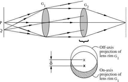
The off-axis behaviour of attenuation is optical in nature, and is the result of the intrinsic optical construction and design. In contrast, vignetting is caused by partial obstruction of light from the object space to image space. The obstruction occurs because the cone of light rays from an off-axis source to the entrance pupil may be partially cut off by the field stop or by other stops or lens rim in the system.
}
xx
P Q
G 1
Off-axis projection of lens rimG
1
On-axis projection of lens rimG
1
δ
G 2
Fig. 2.Geometry involved in vignetting. Note that here there exists a physical stop. Contrast this with Figure 1, where only the effect of off-axis illumination is considered. The geometry of vignetting can be seen in Figure 2. Here, the object space is to the left while the image space is to the right. The loss of light due to vignetting can be expressed as the approximation (see [14], pg. 346)
I
vig(θ)≈(1−αr)I(θ) (7)
This is a reasonable assumption if the off-axis angle is small. In reality, the expression is significantly more complicated in that it involves several other unknowns. This is especially so if we take into account the fact that the off-axis projection of the lens rim is elliptical and the original radius on-axis projection has a radius different from that ofG2in Figure 2.
2.3 Tilting the camera
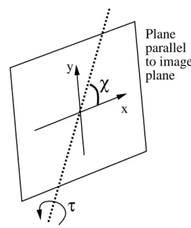
Since the center of rotation can be chosen arbitrarily, we use a tilt axis in a plane parallel to the image plane at an angleχ with respect to the x-axis (Figure 3). The tilt angle is denoted by τ. The normal to the tilted object sheet can be easily shown to be
ˆ
nτ = (sinχsinτ, −cosχsinτ, cosτ)T. (8)
The ray that pass through (u, v) has a unit vector ˆ
nθ= ( u f,vf,1)T
1 + (r f)2
x
y
τ
χ
Plane
parallel
to image
plane
Fig. 3.Tilt parametersχandτ. The rotation axis lies on a plane parallel to the image plane.
The foreshortening effect is thus ˆ
nθ·nˆτ = cosθcosτ
1 +tanf τ(usinχ−vcosχ)
(10) There are two changes to (4), and hence (5), as a result of the tilt:
– Foreshortening effect on local object area dA, wheredAcosθis replaced by
dA(ˆnθ·nˆτ)
– Distance to lens, where (R/cosθ)2 is replaced by (R/(ˆnθ·nˆτ/cosτ))2 This is computed based on the following reasoning: The equation of the tilted object plane, originallyRdistance away from the center of projection, is
p·nˆτ = (0,0, R)T·nˆτ =Rcosτ (11)
The image point (u, v), whose unit vector in space is nθ, is the projection
of the pointRτnθ, whereRτ is the distance of the 3-D point to the point of
projection. Substituting into the plane equation, we get
Rτ =Rnˆcosτ
θ·nˆτ (12)
Incorporating these changes to (5), we get
I(θ) =I
0(ˆnθ·nˆτ)
ˆ nθ·nˆτ
cosτ 2
=I 0cosτ
1 + tanτ
f (usinχ−vcosχ) 3
cos4θ =I
0γcos4θ=I0γβ from (6).
2.4Putting it all together Combining (13) and (7), we have
I
all(θ) =I0(1−αr)γβ (14) We also have to take into consideration the other camera intrinsic parameters, namely the principal point (px, py), the aspect ratioa, and the skews. (px, py) is
specified relative to the center of the image. If (uorig, vorig) is the original image location relative to the camera image center, then we have
u v
=
1s
0a uvorigorig
−
px py
(15) The objective function that we would like to minimize is thus
E=
ij
I
all,ij(θ)−I0(1−αr)γβ 2 (16) Another variant of this objective function we could have used is the least median squared metric.
3 Experimental results
The algorithm implemented to recover both the camera parameters and the off-axis attenuation effects is based on the downhill Nelder-Mead simplex method. While it may not be efficient computationally, it is compact and very simple to implement.
3.1 Simulations
The effects of off-axis illumination and vignetting are shown in Figure 4 and 5. As can be seen, the drop-off in pixel intensity can be dramatic for short focal lengths (or wide fields of view) and significant vignetting effect. Our algorithm depends on the dynamic range of pixel variation for calibration, which means that it will not work with cameras with a very small field of view.
There is no easy way of displaying the sensitivity of all the camera parameters to intensity noise σn and the original maximum intensity levelI0 (as in (14)). In our simulation experiments, we ran 50 runs for each value of σn and I0. In each run we randomize the values of the camera parameters, synthetically
(a) (b) (c)
Fig. 4.Effects of small focal lengths (large off-axis illumination effects) and vignetting: (a) image with f = 500, (b) image withf = 250, and (c) image with f = 500 and α= 1.0−3. The size of each image is 240×256.
0 100 200
X coordinate (pixel)
0 50 100 150 200 250
Intensity
f = 1000 f = 500 f = 250
0 100 200
X coordinate (pixel)
0 50 100 150 200 250
Intensity
α = 0.0 α = 0.0001 α = 0.0005 α = 0.001
(a) (b)
Fig. 5. Profiles of images (horizontally across the image center) with various focal lengths and vignetting effects: (a) varyingf, (b) varyingα(atf=500).
generate the appearance of the image, and use our algorithm to recover the camera parameters. Figure 6 shows the graphs of errors in the focal length f, location of the principal pointp, and the aspect ratioa. As can be seen,f anda
are stable under varyingσnandI0, while the error inpgenerally increases with increasing intensity noise. The error inpis computed relative to the image size.
0.0 0.5 1.0 1.5 2.0
Intensity noise
0.0 2.0 4.0 6.0 8.0 10.0
% error in f
I_0 = 255 I_0 = 200 I_0 = 155
0.0 0.5 1.0 1.5 2.0
Intensity noise
0.0 2.0 4.0 6.0 8.0 10.0
% error in p
I_0 = 255 I_0 = 200 I_0 = 155
(a) (b)
0.0 0.5 1.0 1.5 2.0
Intensity noise
0e+00 1e−05 2e−05 3e−05 4e−05 5e−05
Absolute error in a
I_0 = 255 I_0 = 200 I_0 = 155
(c)
Fig. 6.Graphs of errors in selected camera parameters across different maximum inten-sityI0and intensity errors: (a) focal lengthf, (b) principal point location, (c) absolute
error in aspect ratio.
3.2 Experiments with real images
We also used our algorithm on real images taken using two cameras, namely the Sony Mavica FD-91 and the Sharp Viewcam VL-E47. We conducted our experiments by first taking a picture of a known calibration pattern and then
taking another picture of a blank paper in place of the pattern at the same camera pose. The calibration pattern is used to extract camera parameters as a means of “ground truth.” Here, calibration is done using Tsai’s algorithm [15]. Note that the experiments were conducted under normal conditions that are not highly controlled.
The results are mixed: The focal length estimated using our proposed tech-nique range from 6% to 50% of the value recovered using Tsai’s calibration technique. The results tend to be better for images taken at wider angles (and hence more pronounced off-axis illumination dropoff effects). It is also interesting to find that the focal length estimated using our method is consistently under-estimated compared to that under-estimated using Tsai’s algorithm. What is almost universal, however, is that the estimation of the principal point and camera tilt using our method is unpredictable and quite often far from the recovered “ground truth.”However, we should note that Tsai’s calibration method for a single plane does not produce a stable value for the principal point when the calibration plane is close to being fronto-parallel with respect to the camera.
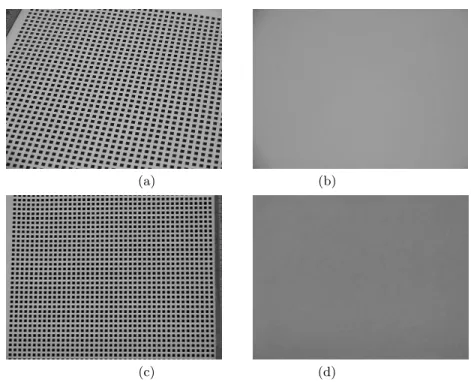
(a) (b)
(c) (d)
Fig. 7. Two real examples: images of calibration pattern (a,c) and their respective “blank” images (b,d). The image size for (a,b) is 512×384 while that for (c,d) is 640×486.
In this paper, we describe two of the experiments with real images. In experi-ment 1, the images in Figure 7(a,b) were taken with the Sony Mavica camera. In
experiment 2, the images in Figure 7(c,d) were taken with the Sharp Viewcam camera. Notice that the intensity variation in (d) is much less than that of (b). Tables 1 and 2 summarize the results for these experiments. Note that we have converted Tsai’s Euler representation to ours for comparison. Our values are quite different from those of Tsai’s. There seems to be some confusion between the location of the principal point and the tilt parameters.
Ours Tsai’s f (pixels) 1389.0 1488.9
κ — 3.56×10⁻⁸
a 0.951 1.0
p (-4.5, 18.8) (37.8, 14.7)
χ 1.8o 2.1o
τ −0.3o −40.0o
Table 1. Comparison between results from our method and Tsai’s calibration for Experiment 1.κis the radial distortion factor,pis the principal point,ais the aspect ratio, andχandτ are the two angle associated with the camera tilt.
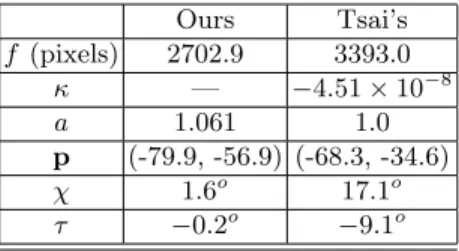
Ours Tsai’s
f (pixels) 2702.9 3393.0
κ — −4.51×10⁻⁸
a 1.061 1.0
p (-79.9, -56.9) (-68.3, -34.6)
χ 1.6o 17.1o
τ −0.2o −9.1o
Table 2. Comparison between results from our method and Tsai’s calibration for Experiment 2.κis the radial distortion factor. Note that in this instance, the calibration plane is almost parallel to the imaging plane.
4 Discussion
In our work, we ignored the effect of radial distortion. This is for the obvious reason that its radial behaviour can misguide the recovery of off-axis drop-off parameters, which have radial behaviour as well. In addition, shadows, and pos-sibly interreflection, will have a deleterious result on our algorithm. As a result, it is easy to introduce unwanted and unmodeled effects in the image acquisition process.
0 100 200 300 400 500 600
X coordinate (pixel)
0 50 100 150 200 250
Intensity
Original distribution Best fit distribution
0 100 200 300 400 500 600
X coordinate (pixel)
0 50 100 150 200 250
Intensity
Original distribution Best fit distribution
(a) (b)
Fig. 8.Actual and fit profiles for the examples shown in Figure 7. (a) corresponds to Figure 7(a,b) while (b) corresponds to Figure 7(c,d).
The dynamic range of intensities is also important in our algorithm; this is basically a signal-to-noise issue. It is important because of the intrinsic errors of pixel intensity due to the digitization process. In a related issue, our algorithm works more reliably for wide-angled cameras, where the off-axis illumination and vignetting effects are more pronounced. This results in a wider dynamic range of intensities. One problem that we have faced in our experiments with real images is that one of our cameras used (specifically the Sony Viewcam) has the auto-iris feature, which has the unfortunate effect of globally dimming the image intensities.
Another unanticipated issue is that if paper is used and the camera is zoomed in too significantly, the fiber of the paper becomes visible, which adds to the texture in the resulting image. It is also difficult to have uniform illumination under normal, non-laboratory conditions.
On the algorithmic side, it appears that it is relatively easy to converge on a local minimum. However, if the data fit is good, the results are usually close to the values from Tsai’s calibration method, which validates our model. We should also add that the value of the principal point cannot be stably recovered using Tsai’s single-plane calibration method when the calibration plane is close to being fronto-parallel with respect to the camera. Our use of a simplified vignetting term may have contributed significantly to the error in camera parameter recovery.
We do admit that our calibration technique, in its current form, may not be practical. However, the picture may be radically different if images were taken under much stricter controls. This is one possible future direction that we can undertake, in addition to reformulating the vignetting term.
5 Conclusions
We have described a calibration technique that uses only the image of a flat textureless surface under uniform illumination. This technique takes advantage of the off-axis illumination drop-off behaviour of the camera. Simulations have shown that both the focal length and aspect ratio are robust to intensity noise and original maximum intensity. Unfortunately, in practice, under normal con-ditions, it is not easy to extract highly accurate camera parameters from real images. Under our current implementation, it merely provides a ballpark figure of the focal length. We do not expect our technique to be a standard technique to recover camera parameters accurately; there are many other techniques for that. What we have shown is that in theory, camera calibration using flat tex-tureless surface under uniform illumination is possible, and that in practice, a reasonable value of focal length can be extracted. It would be interesting to see if significantly better results can be extracted under strictly controlled conditions.
References
1. S. Avidan and A. Shashua. Novel view synthesis in tensor space. InConference on Computer Vision and Pattern Recognition, pages 1034–1040, San Juan, Puerto Rico, June 1997.
2. D. C. Brown. Close-range camera calibration. Photogrammetric Engineering, 37(8):855–866, August 1971.
3. O. D. Faugeras. What can be seen in three dimensions with an uncalibrated stereo rig? InSecond European Conference on Computer Vision (ECCV’92), pages 563– 578, Santa Margherita Liguere, Italy, May 1992. Springer-Verlag.
4. R. Hartley. In defence of the 8-point algorithm. In Fifth International Confer-ence on Computer Vision (ICCV’95), pages 1064–1070, Cambridge, Massachusetts, June 1995. IEEE Computer Society Press.
5. R. Hartley, R. Gupta, and T. Chang. Estimation of relative camera positions for uncalibrated cameras. In Second European Conference on Computer Vision (ECCV’92), pages 579–587, Santa Margherita Liguere, Italy, May 1992. Springer-Verlag.
6. R. I. Hartley. An algorithm for self calibration from several views. In IEEE Computer Society Conference on Computer Vision and Pattern Recognition (CVPR’94), pages 908–912, Seattle, Washington, June 1994. IEEE Computer So-ciety.
7. M. V. Klein and T. E. Furtak. Optics. John Wiley and Sons, 1986.
8. J. J. Koenderink and A. J. van Doorn. Affine structure from motion. Journal of the Optical Society of America A, 8:377–385538, 1991.
9. H. C. Longuet-Higgins. Acomputer algorithm for reconstructing a scene from two projections. Nature, 293:133–135, 1981.
10. P. Mouroulis and J. Macdonald. Geometrical optics and optical design. Oxford University Press, 1997.
11. M Pollefeys, R. Koch, and Van Gool L. Self-calibration and metric reconstruction in spite of varying and unknown internal camera parameters. In International Conference on Computer Vision (ICCV’98), pages 90–95, Bombay, India, January 1998. IEEE Computer Society Press.
12. A. Shashua. Projective structure from uncalibrated images: Structure from motion and recognition.IEEE Transactions on Pattern Analysis and Machine Intelligence, 16(8):778–790, August 1994.
13. G. Stein. Accurate internal camera calibration using rotation, with analysis of sources of error. InFifth International Conference on Computer Vision (ICCV’95), pages 230–236, Cambridge, Massachusetts, June 1995.
14. J. Strong. Concepts of Classical Optics. W.H. Freeman and Co., San Francisco, CA, 1958.
15. R. Y. Tsai. Aversatile camera calibration technique for high-accuracy 3D ma-chine vision metrology using off-the-shelf TV cameras and lenses. IEEE Journal of Robotics and Automation, RA-3(4):323–344, August 1987.
16. A. Zisserman, P. Beardsley, and I. Reid. Metric calibration of a stereo rig. In
IEEE Workshop on Representations of Visual Scenes, pages 93–100, Cambridge, Massachusetts, June 1995.