Do the Rich Save More?
Karen E. Dynan Mail Stop 80
Federal Reserve Board Washington, DC 20551 202-452-2553
Jonathan Skinner Economics Department 301 Rockefeller Hall Dartmouth College Hanover, NH 03755 603-646-2535
Stephen P. Zeldes
Graduate School of Business Columbia University
3022 Broadway, Uris 605B New York, NY 10027-6902 212-854-2492
[email protected] November 2000
Abstract
The issue of whether higher lifetime income households save a larger fraction of their income is an important factor in the evaluation of tax and macroeconomic policy. Despite an outpouring of research on this topic in the 1950s and 1960s, the question remains unresolved and has since received little attention. This paper revisits the issue, using new empirical methods and the Panel Study on Income Dynamics, the Survey of Consumer Finances, and the Consumer Expenditure Survey. We first consider the various ways in which life cycle models can be altered to generate differences in saving rates by income groups: differences in Social Security benefits, different time preference rates, non-homothetic preferences, bequest motives,
uncertainty, and consumption floors. Using a variety of instruments for lifetime income, we find a strong positive relationship between personal saving rates and lifetime
income. The data do not support theories relying on time preference rates,
non-homothetic preferences, or variations in Social Security benefits. Instead, the evidence is consistent with models in which precautionary saving and bequest motives drive variations in saving rates across income groups. Finally, we illustrate how models that assume a constant rate of saving across income groups can yield erroneous
predictions.
We thank Dan Bergstresser, Wynn Huang, Julie Kozack, Stephen Lin, Byron Lutz, and Marta Noguer for research assistance, Orazio Attanasio for help with the CEX data, and Andrew Samwick for help with Social Security data and calculations. Zeldes is grateful for financial support from Columbia Business School and a TIAA-CREF Pension and Economic Research Grant, and Skinner for financial assistance from the National Institute on Aging. We thank Don Fullerton, James Poterba, John Sabelhaus, James Smith, Mark Warshawsky, David Weil, seminar participants at the NBER Summer Institute, the NBER Inter-American Conference, the Universities of Michigan and Maryland, and Georgetown, Harvard, Northwestern, Stanford, and Yale Universities for helpful comments; we are especially grateful to Casey Mulligan for detailed suggestions. The views expressed are those of the authors and not necessarily those of the Federal Reserve Board or its staff. This version is the same as NBER working paper no. 7906 (September 2000).
1 Blinder (1975) finds little connection between shifts in the income distribution and the aggregate
saving rate, but argues that the changes in the income distribution present in postwar U.S. data are unlikely to correspond to the type of pure redistribution required by the theory.
I. Introduction
It would be easy to convince a room full of non-economists that higher lifetime income levels lead to higher saving rates. Non-economists would tell you that low income people can't afford to save. Certainly a room full of journalists would need little convincing: Examples include "A sales tax would shift the tax burden from the rich to the middle class, since affluent people save a much larger portion of their earnings" (Passell, New York Times, 1995), and "The poor and middle class spend a higher percentage of their income on goods than do the rich, and so, according to most economists' studies, a value-added tax is regressive" (Greenhouse, New York Times, 1992).
A room full of economists would be less easily persuaded that higher lifetime income levels lead to higher saving rates. The typical economist would point out that people with temporarily high income will tend to save more to compensate for lower future income, and people with temporarily low income will tend to save less in anticipation of higher future income. Thus, even if the saving rate is invariant with regard to lifetime income, we will observe people with high current incomes saving more than their lower income brethren (Friedman, 1957).
Moreover, the stylized facts about the aggregate U.S. saving rate do not seem to support a positive correlation between saving rates and income. First, there has been no time-series increase in the aggregate saving rate during the past century despite dramatic growth in real per capita income. Second, the increasing concentration of income toward the top income quintile during the 1980s and early 1990s did not lead to higher aggregate saving rates.1 Looking across countries, Schmidt-Hebbel and Serven (2000) found no evidence of a statistically significant link between measures of income inequality and aggregate saving rates.
Despite an outpouring of research in the 1950s and 1960s, the question of whether the rich save more has since received little attention. Much of the early empirical work favored the view that high income people did in fact save a higher
2 One can assume a representative agent because the marginal and average propensities to save
from lifetime income are identical for all individuals in the economy. See Caselli and Ventura (1999) for a more general model in which individual consumption is a linear function of income and wealth, thus retaining desirable aggregation properties.
3 See, for example, Stoker (1986).
fraction of their income (e.g., Mayer, 1966, 1972). However, a sufficient number of studies, by Milton Friedman and others, reached the opposite conclusion to leave “reasonable doubt” about the alleged propensity of high lifetime income households to save more.
We return to the topic of how saving rates vary with lifetime income for two reasons. First, the empirical issues remain somewhat clouded, and a wide variety of newer data sources, such as the Panel Study of Income Dynamics (PSID), the Survey of Consumer Finances (SCF), the Consumer Expenditure Survey (CEX), and work on imputed saving from Social Security and pension contributions (Feldstein and Samwick, 1992; Gustman and Steinmeier, 1989) allow a much richer picture of empirical patterns of saving behavior. Second, we believe that the topic has important implications for the evaluation of economic policy. If Milton Friedman and his collaborators did not earn a clear-cut victory in the empirical battles of the 1960s, they won the war. Many models used for macroeconomic or microeconomic policy evaluation assume that saving is proportional to lifetime resources, which allows the distribution of heterogeneous people with different incomes to be collapsed into a single “representative” agent.2 The Leeper and Sims (1994) macroeconomic policy model, and the work by Auerbach and Kotlikoff (1987) on tax incidence analysis are examples of such models.
The question we are examining bears on a number of important issues. First, a finding of heterogeneous saving rates would suggest that the effects on aggregate consumption of shocks to aggregate income or wealth would depend not only on the magnitude of the shock but also on its distribution across income groups.3 Second, the results could shed light on the debate in the economic growth literature about whether the positive correlation between income and saving rates across countries reflects high saving rates causing high income or vice versa. Third, the results could help us
groups. Fourth, the incidence and effectiveness of reform proposals that shift taxation away from saving (such as value-added taxes, consumption taxes, flat taxes, and expanded IRAs) depend on how much saving is done by each income group. Finally, the question of whether higher income households save at higher rates than lower income households has important implications for the distribution of wealth, both within and across cohorts.
We find first, like previous researchers, a strong positive relationship between current income and saving rates across all income groups, including the very highest income categories. Second, and more important, we continue to find a positive
correlation when we use proxies for permanent income such as education, lagged and future earnings, the value of vehicles purchased, and food consumption. Estimated saving rates range from less than 5 percent for the bottom quintile of the income distribution to more than 40 percent of income for the top 5 percent. The positive relationship is more pronounced when we include imputed Social Security saving and pension contributions. Even among the elderly, saving rates may rise with income. In sum, our results suggest strongly that the rich do save more, whether the rich are defined to be the top 20 percent of the income distribution (following the Department of Treasury -- Pines, 1997), or the top 1 percent. And, more broadly, we find that saving rates increase across the entire income distribution.
These basic patterns of saving are not consistent with the predictions of
standard homothetic life-cycle models. Nor, as we show below, are they consistent with explanations that range from differences in time preference rates or subsistence
parameters to variation in Social Security replacement rates. Rather, we conclude that the data are consistent with a model that emphasizes the dual role for saving later in life: money is set aside for catastrophic expenditures such as a costly illness or other contingency, and, in the likely case that the money is not needed for such an event, it is passed along to heirs (see also Smith, 1999a). This combination of precautionary and bequest motives stimulates saving most for higher income households, and has less effect on lower income households, perhaps because of asset-based means tested social insurance programs, like Medicaid, or less desire to leave financial bequests to subsequent generations (e.g. Becker and Tomes, 1986 and Mulligan, 1997). As well as
explaining the cross-sectional pattern in saving, such a model also implies that steady-state saving rates should remain constant over time despite long-term income growth.
In the next section, we consider models of consumption that allow for systematic differences in saving behavior by lifetime income group. Section III describes the
empirical methodology, focusing on the key issue of identification of permanent income. In Section IV, we describe the three data sets used for the analysis. Our empirical results are in Section V, and Section VI concludes.
II. The Empirical and Theoretical Background
Many economists in previous generations used both theory and empirics to assess whether people with high incomes save more than people with low incomes. Early theoretical contributions include Fisher (1930), Keynes (1936), Hicks (1950), and Pigou (1951); early empirical work includes Vickrey (1947), Duesenberry (1949), Friedman (1957), Friend and Kravis (1957), Modigliani and Ando (1960), and many more.
In his work on the permanent income hypothesis, Friedman (1957) noted that cross-sectional data show a positive correlation between income and saving rates, but argued that this result reflected individuals changing their saving in order to keep consumption smooth in the face of temporarily high or low income. He contended that individuals with high permanent income consume the same fraction of permanent income as individuals with low permanent income, and he emphasized empirical regularities that appeared to support this proportionality hypothesis. Many studies of this hypothesis followed, some supporting Friedman and some not. Evans (1969) summarized the state of knowledge about consumption in 1969, concluding "it is still an open question whether relatively wealthy individuals save a greater proportion of their income than do relatively poor individuals" (p. 14).
In a comprehensive examination of the available results and data, Mayer (1972) disagreed, claiming strong evidence against the proportionality hypothesis. For
example, when he proxied for permanent income and consumption with five-year averages from annual Swiss budget surveys, he found the elasticity of consumption with respect to permanent income to be significantly different from one (0.905), and not
4 See Browning and Lusardi (1996) for a survey of recent micro-level empirical research on
saving.
(1)
much different from the elasticity based on one year of income. Mayer interpreted this result as a rejection of the proportionality hypothesis.
Despite the abundance of early studies on this important question, little work has been done since. The relative lack of interest in part reflects the influential work of Lucas (1976) and Hall (1978), which shifted work away from learning about levels of consumption or saving toward "Euler Equation" estimation techniques that implicitly examine first differences in consumption.4
Some studies have found that wealth levels are disproportionately higher among households with high lifetime income (Diamond and Hausman,1984; Bernheim and Scholz, 1993; Hubbard, Skinner, and Zeldes, 1995). While this result could be explained by higher saving rates among higher income households, it could also be explained by higher rates of return (on housing or the stock market, for example) or the receipt of proportionately more intergenerational transfers by these households. Others have argued that wealth levels when properly measured are not disproportionately higher among high income households. Gustman and Steinmeier (1999) and Venti and Wise (1998) augmented conventionally measured wealth with imputed Social Security and pension wealth from the Health and Retirement Survey; they found that the ratio of this augmented wealth to lifetime earnings (based on lengthy Social Security records) was constant or even declining with lifetime earnings. As we show below, these seemingly contradictory results illustrate the importance of how one measures lifetime income and the distinction between flows (saving) and stocks (wealth).
To help make the question more precise, consider a life-cycle / permanent income model with a bequest motive. At each age t, households maximize expected lifetime utility
where E is the expectation operator, C*
5 Note that since r includes the total return to non-human wealth including capital gains, saving
measured as income minus consumption is identical to saving measured as the change in wealth. We return to this issue below.
(2)
(3)
time s,
*
i is the household-specific rate of time preference, Bis is the bequest left in the event of death, and V("
) is the utility of leaving a bequest. To allow for mortality risk,B
is is the probability (as of time t) of dying in period s, Dis is a state variable that is equal to one if the household is alive through period s and zero otherwise, and T is themaximum possible length of life.
The family begins period s with net worth (exclusive of human wealth)
Ais-1(1+ris-1), where ris-1 is the real after-tax rate of return on non-human wealth between s-1 and s. We assume that there are no private annuity markets. The family first learns about medical expenses (Mis), which we treat as necessary consumption that generates no utility. It next receives transfers (TRis) from the government. It then learns whether it survives through the period. If not, it leaves to heirs a non-negative bequest,
If it survives, the household receives after-tax earnings (Eis) and chooses non-medical consumption. We define total consumption as Cis
/
C*is + Mis. End of period wealth (Ais) is thus:We define real annual income Yis
/
ris-1 Ais-1 + Eis + TRis, and saving as Sis/
Yis - Cis =Ais - Ai s-1.5
Define lifetime resources (as of period s) as period s non-human wealth plus the expected present value of future earnings and transfers. Under what circumstances will consumption (and saving) be proportional to lifetime resources? In a world with no uncertainty and no bequest motive, two sets of assumptions will generate
proportionality in consumption. First, if the rate of time preference (
*
i) and the rate of return (ris) are constant and equal to each other, any separable utility function will yield constant consumption over the lifetime, equal to the appropriate annuity factor6 Adding uncertainty complicates the model, but again two sets of assumptions will generate the
result that consumption rises proportionately with the scale factor for earnings. First, if the utility function is quadratic and *i and ris are constant and equal to each other, consumption will be proportional to the
expected value of lifetime resources, as defined above. If the utility function is not quadratic then there is no single summary statistic that defines consumption. However, if one assumes the utility function is isoelastic and initial wealth and all possible realizations of earnings are scaled up by a constant factor, then consumption will also be scaled up by that factor and saving rates will be identical (Bar-Ilan, 1995).
7 Our discussion and empirical estimates focus on differences in the average propensity to save
across income levels. Some, but not all, of the explanations below would also generate differences in the marginal propensity to save.
8 The only purpose of the third period is to allow for medical expenses late in life – we assume no
non-medical consumption in this period.
multiplied by lifetime resources. Second, if preferences are homothetic, i.e. the utility function is isoelastic: U(C) = (C1-( -1)/(1-
(
), consumption will be proportional to lifetimeresources. If all households have the same preference parameters and face the same interest rates, then the constant of proportionality will be the same for all households. If one further assumes that the initial wealth and the age-earnings (and age-transfers) profiles of rich households are simply scaled-up versions of those for poor households, then the proportionality in consumption implies that saving rates will be identical across households.6
How then could saving rates differ across income groups? We consider three general classes of models: one encompasses certainty models without a bequest motive, the second allows for uncertainty with respect to future income or health
expenses (but no bequest motive), and the third includes an operative bequest motive.7 To provide illustrative calculations of how saving rates differ across income
groups in these classes of models, we present results from a simple three-period version of the model above. We think of period one (“young”) as ages 30-60, period two (“old”) as ages 60-90, and period three as the time around death (when old) when medical expenditures are paid and bequests are left.8 We assume an isoelastic utility function with
(
= 3, a value consistent with previous studies. Further details are provided below.A. Consumption models with no uncertainty and no bequest motive
9 We set the probability of living to old age (period 2) at 82 percent, based on statistics from the
Berkeley mortality database; http://demog.berkeley.edu/wilmoth/mortality/overview.html. Since period 3 represents the very end of life, all households that survive to period 2 die in period 3.
10 Other examples (for which similar exercises could be performed) include: 1) differences in the
timing of earnings (higher income households tend to have a steeper age-earnings profile, inducing them to save less when young than lower income households), 2) differences in life expectancy (higher income households tend to live longer, inducing them to save more when young than lower income households), or 3) differences in retirement age (higher income households tend to retire later, inducing them to save less when young).
about the length of life.9 We examine two income groups, low income and high income, with assumed average first-period income of $16,116 and $75,000, based on the 20th and 80th percentile of the income distribution in 1998 (U.S. Census, 1999). We assume that in the second period Social Security and pension income replace 60 percent of pre-retirement (or first-period) income, consistent with the overall replacement rate in
Gustman and Steinmeier (1999). The (annual) rates of time preference and interest are 0.02 and 0.03, respectively, which, together with uncertain lifespan, result in a roughly flat pattern of non-medical consumption over the lifetime.
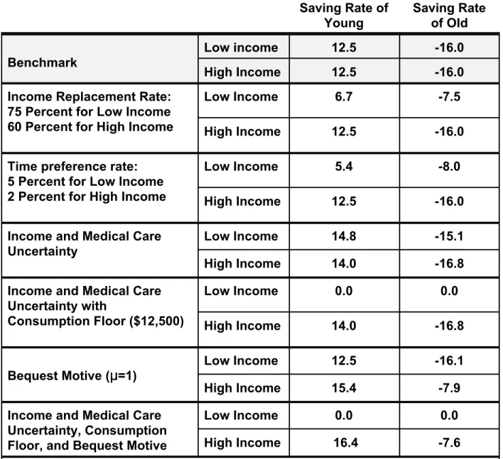
In table 1, we present the predicted saving rates for working age (young) and retirement age (old) households. The results are identical for the low income and high income groups, with saving rates while young equal to 12.5 percent in addition to pensions and Social Security, and dissaving rates while old equal to 16.0 percent.
In the standard life cycle model, there are two approaches to generating higher saving rates for higher income households: differences in the timing of income for these households and differences in the timing of consumption. We consider each in turn.
Differences in the timing of earnings and transfers across lifetime income groups will yield different patterns of saving despite identical slopes of the consumption paths. For example, Social Security programs typically provide a higher replacement rate for low income households and thus reduce the need for these households to save for retirement (e.g., Huggett and Ventura, 2000; Smith, 1999a).10 We consider the effects in our model of increasing the replacement rate for the low income households from 60 percent to 75 percent (and increasing first period Social Security taxes for these
households such that the present value of lifetime resources is unaffected). Table 1 shows that the saving rate while young falls, to just 6.7 percent. Saving rates while old
Table 1: Simulated Saving Patterns Saving Rate of
Young
Saving Rate of OId Benchmark
Low income 12.5 -16.0
High Income 12.5 -16.0
Income Replacement Rate: 75 Percent for Low Income 60 Percent for High Income
Low Income 6.7 -7.5
High Income 12.5 -16.0
Time preference rate: 5 Percent for Low Income 2 Percent for High Income
Low Income 5.4 -8.0
High Income 12.5 -16.0
Income and Medical Care
Uncertainty Low Income 14.8 -15.1
High Income 14.0 -16.8
Income and Medical Care Uncertainty with
Consumption Floor ($12,500)
Low Income 0.0 0.0
High Income 14.0 -16.8
Bequest Motive (
:
:
=1)Low Income 12.5 -16.1
High Income 15.4 -7.9
Income and Medical Care Uncertainty, Consumption Floor, and Bequest Motive
Low Income 0.0 0.0
High Income 16.4 -7.6
Default parameters: 2 percent time preference rate, 82 percent chance of surviving to be “old,” 60 percent replacement rate, 3 percent interest rate.
11 Define Social Security saving equal to the present value of future Social Security benefits
accrued as a result of Social Security contributions in period 1. The modified saving rate adds Social Security saving to both the numerator (saving) and the denominator (income).
12 This assumes that consumption would be unaffected by the change. If this “forced saving”
lowered the consumption while young, it would raise the comprehensive saving of low income households.
13 Lawrance (1991) offers empirical evidence to this effect, although Dynan (1994) shows that the
patterns are not pronounced after controlling for ex-post shocks to income. See also Bernheim, Skinner, and Weinberg (1997).
increase to -7.5 percent. In other words, if lower income households have higher retirement replacement rates then they will save less while working, and dissave less while retired. Suppose that we were to instead construct a more comprehensive saving rate inclusive of “Social Security saving”.11 This saving rate would equal 12.5 percent, identical to the saving rate for high income households.12 In other words, if a Social Security program of the type presented here is causing saving rates to decline with income, the comprehensive saving rate would show no such decline. We construct this comprehensive saving measure in our empirical work below. Note that if we were to change the model so that the Social Security program provided future benefits to low income households greater (in present value) than the contributions (making it
progressive), then the comprehensive saving measure would show saving rates of the low income working households that were greater than saving rates of the high income households.
Next consider differences in the timing of consumption. If high income households choose more rapid growth rates in consumption, they will have higher saving rates, at least at younger ages.13 For example, a negative relationship between the time preference rate
*
and the level of income could lead higher incomehouseholds to have steeper consumption paths. This might happen in a world with imperfect capital markets because households with lower time preference rates would have a greater inclination toward saving (when young) and would also be more likely to have higher earnings because of greater investment in education and other forms of
14 With perfect capital markets, households with high time preference would borrow to finance
their education, yielding no relationship between time preference and years of schooling or earnings. See, for example, Cameron and Taber (2000).
15 In this type of model, a third factor (the rate of time preference) is causing both the higher
permanent income and the higher saving rate. (See, for example, Evans and Montgomery, 1995, on the correlation between different types of forward-looking behavior.) Therefore, exogenously raising the permanent income of a given household would not raise its saving rate. See Mayer (1972) for further discussion.
16 Differences across lifetime income groups in the number and/or timing of children could also
generate differences in the timing of consumption. See Attanasio and Browning (1995) for work relating consumption and family size.
17 Although the need to meet the current subsistence level depresses the saving rate of lower
income households, the need to meet future requirements boosts the saving rate of those households. The net effect depends (in a certainty model) on the relative magnitudes of r and *. Because of the subsistence level, poor households will be on a more steeply sloped portion of their utility functions than rich households. As a result, they will be less willing to substitute consumption over time and will have flatter consumption paths. If r > *, the consumption paths of both rich and poor households will slope upward, and the flatter paths of poor households will be associated with lower saving rates when young. If r < *, the reverse is true: consumption paths will slope downward, and the flatter path of the poor will be associated with a higher saving rate when young. A different way to generate the result that higher
human capital.14,15 Alternatively, Becker and Mulligan (1997) suggest that the causality may run the other way, with a higher level of income encouraging people to invest resources that make them more farsighted. In either case, the level of lifetime earnings would be positively correlated with both the growth rate of consumption and saving rates while young.16
Turning back to our model, suppose that low income households have an
(annual) time preference rate of 0.05, instead of 0.02. Table 1 shows that the resulting saving patterns look very much like those when the income replacement rate is higher for these households. For low income households, the saving rate while young drops to 5.4 percent, and the saving rate while old falls to -8.0 percent. Once again, we see higher saving by higher income households while young but more dissaving while old.
One can also generate income-based differences in consumption growth rates by assuming a “subsistence” or necessary level of consumption. Informal arguments are sometimes made that subsistence levels imply that poor households have lower saving rates because they cannot “afford to save” after buying the necessities. However, this result requires that r >
*
; if r <*
, a subsistence level of consumption causes rich households to save less than poor households.17 Closely related areincome households have higher saving rates is to assume that subsistence levels decline with age.
18 This result presumes that substitution effects dominate income effects; see Elmendorf (1996).
Note also that higher income households face higher marginal tax rates, lowering their after-tax return.
19 Thaler (1994) and Laibson (1997) describe a class of models in which preferences are
dynamically inconsistent. Consumers’ desire for a high saving path is undermined by a preference for immediate gratification. The illiquidity of housing equity and pensions allows consumers to commit to higher saving rates.
20 This degree of uncertainty is consistent with empirical parameterizations of earnings variability
(e.g., Hubbard, Skinner, and Zeldes, 1994).
models in which the intertemporal elasticity of substitution is larger for high income households (Attanasio and Browning,1995; Atkeson and Ogaki, 1996; and Ogaki, Ostry, and Reinhard, 1996).
Finally, the pattern could arise if higher income households enjoy better access to investment opportunities, such as equity markets, pensions, and housing. This may provide them with a higher rate of return (Yitzhaki, 1987),18 or a better mechanism to overcome their preferences for immediate gratification, as in Thaler (1994) and Laibson (1997).19 In sum, differences in the timing of income and differences in the timing of consumption can explain higher saving among higher income households while young, but they also imply that these households have higher dissaving rates when old.
B. Consumption models with uncertainty but no bequest motive
Does the precautionary motive for saving imply that high income households should save more? To answer this question, we incorporate two additional sources of uncertainty in the model. First, we allow for risk to second-period income that might be associated with earnings shocks, forced early retirement, or the loss of a spouse. We assume a discretized distribution with an equal chance of earnings either one-quarter higher or one-quarter lower than in the case of perfect certainty.20
Second, we allow for the possibility of large medical expenses, especially near death. For example, Hurd and Wise (1989) found a decline in median wealth of $103,134 (in 1999 dollars) for couples suffering the death of a husband, and Smith (1999b) found that wealth fell following severe health shocks, by $25,371 for
households above median income and by $11,348 for families below median income. Covinsky et al (1994) found that 20 percent of a sample of families experiencing a
21 On the other hand, Hurd and Smith (1999) find smaller median changes in wealth near death. 22 We assume that the household learns about the size of medical expenses prior to choosing
second-period consumption, but does not pay the expenses until period 3.
death from serious illness reported that the illness had essentially wiped out their assets.21
For simplicity, we subtract medical expenditures from earnings (so that our earnings are net of health care expenditures) in the first two periods, and focus on uncertainty about health care expenditures only in the final period, at the very end of life. We assume health expenditures of $60,000 with 20 percent probability, and $0 otherwise.22 We compute the average saving rate in period 2 as average saving divided by average income.
Table 1 shows that when these types of uncertainty are added, saving rates for low income households are larger than for high income households. This is because the income uncertainty is proportional to income (raising saving rates equally for both groups) and the health expenditures represent a higher fraction of lifetime income for these households. Thus, the introduction of these factors alone cannot explain why the rich save more.
More realistically, asset-based means-tested programs such as Medicaid or SSI may reduce the necessity of saving against such contingencies for lower income
households (Hubbard, Skinner, and Zeldes, 1995). Higher income households find the consumption floor less palatable and thus continue to save against future
contingencies. To see the implications, we add a $12,500 means-tested consumption floor to the model: transfers in period 2 are adjusted so as to insure that the household will, after exhausting its other resources, be able to consume $12,500 in the second period and pay for medical expenditures in the final period. Because the household receives these transfers only after spending all other assets, a high chance of becoming eligible for transfers translates into low saving rates while young. Table 1 shows that these programs lead low income households to have zero saving when young (despite the fact they may well not end up on welfare), and dissave nothing when older. In short, the precautionary saving model with asset-based means testing implies
23 An alternative model is one in which wealth per se gives utility above and beyond the flow of
consumption it enables (Carroll, 2000).
low saving rates among lower income households at all ages, with conventional (and substantial) saving rates among high income households.
C. Consumption models with a bequest motive
Thus far, our model has produced only bequests that do not generate utility for the household -- sometimes referred to as unintended or accidental bequests. Here we consider an operative bequest motive as in Becker and Tomes (1986) or Mulligan (1997). Suppose that individuals value the utility of their children and that earnings are mean-reverting across generations. In this case, Friedman's permanent income
hypothesis effectively applies across generations: a household with high lifetime income will save a higher fraction of its lifetime income in order to leave a larger bequest to its offspring who are likely to be relatively worse off.23
We implement this model by specifying an operative bequest function V(Bis) =
:
((Bis + YLcis)1-( - 1)/(1-(
), where:
is the tradeoff parameter between own consumption and bequests, and YLcis is the value of the next generation’s lifetime earnings. We assume complete mean reversion of earnings, so that earnings of the children are equal to the average earnings of parents, and
:
= 1.0.Saving rates in this bequest model (without income or medical care uncertainty) are shown in Table 1. Saving rates while young and old are higher for the higher income group, where the bequest motive is operative. By contrast, lower income households expect their children to have earnings higher than theirs, and so consume their overall resources, yielding saving rates that are the same as for the life cycle model.
Finally, we consider a model with income and medical care uncertainty, a
consumption floor, and an operative bequest motive. Here, bequests are conditional on the health and income draws, so in the good states of the world, the family leaves a much larger bequest than in the bad states of the world. For the high income
household, the saving rate is 16.4 percent when young and -7.6 percent when old. For the low income household, the saving rate is essentially zero for both periods because
of the asset-based means testing. Note that high-income saving rates with both precautionary saving and a bequest motive are not that much larger than either in isolation; this is because the saving is used for bequests in the good state of the world, and for health expenses in the (uncommon) bad state of the world.
III. Empirical Methodology
Three key issues arise in designing and implementing empirical tests. The first is how to define saving. One approach is to consider all forms of saving including realized and unrealized capital gains on housing, financial assets, owner-occupied businesses, and other components of wealth. (These capital gains should also be added to income to be consistent with the Haig-Simon definition of full income.) An alternative is to examine a definition of saving that focuses on the “active” component --that is, the difference between income exclusive of capital gains, and consumption. This would be the relevant one if households do not entirely “pierce the veil” of their saving through capital gains, or if all capital gains are unanticipated at the time the saving decision is made.
Unfortunately, neither definition of saving is clearly superior -- it depends on the question of interest. For example, capital gains should be included when measuring the adequacy of saving for retirement, but excluded when measuring the supply of loanable funds for new investment. We thus construct several measures of saving: the flow of
disposable income less consumption from the CEX, the change in wealth from the SCF and PSID, and the change in wealth exclusive of capital gains and (sometimes)
inclusive of imputed Social Security and pension saving from the PSID.
The second and third key issues are how to distinguish those with high lifetime income from those whose income is high only transitorily and how to correct for
measurement error in income. As Friedman pointed out, these issues are intertwined: "in any statistical analysis errors of measurement will in general be indissolubly merged with the correctly measured transitory component" of income (Friedman, 1957, p. 29). When we measure saving as the residual between income and consumption,
24 Assuming a degree of independence of the measurement errors in Y and C.
25 For early analyses using education as a proxy for permanent income, see Zellner (1960) and
Modigliani and Ando (1960). See Mayer (1972) for a discussion of how heterogeneity in tastes for saving can affect tests of the proportionality hypothesis.
26 If some households face binding liquidity constraints, however, consumption may be correlated
with transitory income.
of the same sign in saving (Y - C).24 Therefore, measurement error in income, like transitory income, can induce a positive correlation between measured income and saving rates even when saving rates do not actually differ across groups with different lifetime resources. A bias arises in the other direction when we define saving as the change in wealth: measurement error in income enters only in the denominator, inducing a negative correlation between measured income and the saving rate.
To reduce the problems associated with measurement error and transitory income, we use proxies for permanent income -- an approach with a long history (Mayer, 1972). We consider four instruments: consumption (total or some components), lagged labor income, future labor income, and education. A good instrument for permanent income should satisfy two requirements. First, it should be highly correlated with true “permanent” or anticipated lifetime income at the time of the saving decision. Second, the instrument should be uncorrelated with the error term, which includes measurement error and transitory income, so that it affects saving rates only through its influence on permanent income.
All of our instruments are likely to satisfy the first requirement. What about the second requirement? The longer the lags used and the less persistent is transitory income, the more likely that lagged and future labor income will be uncorrelated with transitory income. Education is appealing in this regard, because it is well measured and stays constant over time, which minimizes its correlation with transitory income. It may, however, be correlated with tastes toward saving (another possible component of the error term), or have an independent effect on saving (e.g. people may learn how to plan or about the merits of using tax-deferred saving vehicles).25 Since consumption reflects permanent income in standard models, it should be uncorrelated with transitory income, and thus be an excellent instrument (see, e.g., Vickrey, 1947).26 Measurement
error in consumption and transitory consumption will bias the estimated relationship between saving rates and permanent income toward being negative. However, this bias need not invalidate our findings. A finding that measured saving rates rise with measured consumption, despite the induced bias in the opposite direction, would represent strong evidence that saving rates rise with permanent income.
Most of our results are based on a two-stage estimation procedure. In the first stage, we regress current income on proxies for permanent income and age dummies. We then use the fitted values from the first-stage regression to place households into predicted permanent income categories (typically quintiles). In the second stage, we estimate a median regression, with the saving rate as the dependent variable and the predicted permanent income quintiles and age dummies as the independent variables. We use this procedure in order to allow for non-linearities in the relationship between saving rates and lifetime income. We construct standard errors for the estimated saving rates by bootstrapping the entire two-step process. Separately, we also use fitted permanent income (instead of fitted quintiles) as the independent variable in the second stage, both to summarize the relationship between the variables and to provide a simple test of whether it is positive.
IV. Data
Using the CEX, the SCF, and the PSID not only allows for different measures of saving, but also ensures that our conclusions are not unduly influenced by the
idiosyncracies of a single data source. For our pre-retirement analysis, we focus on households between the ages of 30 and 59 (as of the midpoint of their participation in each sample), with younger households excluded because they are more likely to be in transitional stages or students. To analyze the saving behavior of older households, we focus, in the CEX and SCF, on households aged 70 to 79. This reduces the potential problems associated with comparing households before and after retirement as well as the complications that arise for much older households. For the PSID, we examine households ages 62 and older, but also consider a subset of retired households.
27 Attanasio (1994) provides a comprehensive analysis of U.S. saving rate data based on the
CEX.
28 Sabelhaus (1992) and Nelson (1994b) warn that the data on household tax payments are quite
poor. Sabelhaus (1992) suggests estimating these payments with income and demographic information, but we did not attempt to do so. Inaccurate tax data will only bias our results if the degree of inaccuracy is correlated with our instruments for permanent income.
A. Consumer Expenditure Survey (CEX)
The CEX has the best available data on total household consumption.27 In each quarter since 1980, about 5000 households have been interviewed; a given household remains in the sample for four consecutive quarters and then is rotated out and
replaced with a new household. The survey asks for information about consumption, demographics, and income.
We define the saving rate for a CEX household as the difference between consumption and after-tax income, divided by after-tax income (all in 1989 dollars). Consumption equals total household expenditures plus imputed rent for homeowners
minus mortgage payments, expenditures on home capital improvements, life insurance payments, and spending on new and used vehicles. This definition includes
expenditures for houses and vehicles as part of saving, in part in order to make the measure of saving in the CEX closer to those in the PSID and SCF. We use Nelson’s (1994a) reorganization of the CEX, which sums consumption across the four interview quarters for households in the 1982 through 1989 waves. After-tax income equals pre-tax income for the previous year less taxes for this period, as reported in each household's final interview.28 We deflate both income and consumption with price indexes based in 1989. Appendix A includes the definitions of all other variables we use.
We exclude households with nonpositive disposable income so that negative saving rates occur only when consumption exceeds income. We also exclude households with income below $1000, as well as households with invalid income or missing age data, and households who did not participate for all of the interviews. We are left with 14,180 households for our analysis.
B. Survey of Consumer Finances (SCF)
29 We had some concern that the mix of defined benefit versus defined contribution pension
saving could vary with income, so that omitting one but including the other might bias our results. We therefore also examined net worth exclusive of defined contribution pension plans, and the results were similar.
30 Our SCF data set actually contains 2643 observations because each household's data is
repeated three times with different random draws of imputed variables, in order to more accurately represent the variance of the imputed variables. Thus, the standard errors in our analysis must be corrected for the presence of replicates. We do so by multiplying them by 1.73 — the square root of the number of replicates (three).
surveyed in 1983 and then again in 1989. The sample has two parts: households from an area-probability sample and households from a special high-income sample
selected based on tax data from the Internal Revenue Service. The SCF contains very high quality information about assets and liabilities, as well as limited data on
demographic characteristics, and income in the calendar year prior to the survey. The saving rate variable used for the SCF calculations equals the change in real net worth between 1983 and 1989 divided by six times 1988 total real household
income (all variables measured in 1989 dollars). Because it spans several years, this variable is likely to be a less noisy measure of average saving than a one-year
measure. Net worth is calculated as the value of financial assets (including the cash value of life insurance and the value of defined contribution pension plans), businesses, real estate, vehicles and other nonfinancial assets, minus credit card and other
consumer debt, business debt, real estate debt, vehicle debt and other debt. Although, in principle, one could calculate the value of defined benefit pension plans and add them to net worth, we do not attempt to do so.29
We restrict the SCF sample in several ways. First, we exclude households with 1982 or 1988 income less than $1000. Second, we eliminate households where the head or spouse changed between 1983 and 1989 because such changes tend to have dramatic and idiosyncratic effects on household net worth. The resulting sample contains information on 881 households.30
C. Panel Study of Income Dynamics (PSID)
The PSID is the longest running U.S. panel data set, and, as such, it provides a valuable resource unavailable to researchers in the 1950s and 1960s. The long earnings history for each household helps us disentangle transitory and permanent
31 Capital gain in housing is the difference in net equity in the main home between 1984 and 1989
less the cost of additions and repairs made to the home between 1984 and 1989. These gains are restricted to those years in which the family did not move. Financial capital gain equals the change in the value of other real estate, farms, businesses, and stocks between 1984 and 1989 less net financial investment (i.e. the net amount invested in these assets over this period.) We do not correct the active saving variable for inflation.
income shocks, thus facilitating the key issue of identification.
For the asset supplements in 1984 and 1989, net worth is calculated as the sum of the value of checking and savings accounts, money market funds, CDs, government saving bonds, T-bills, and IRAs; the net value of: stocks, bonds, rights in a trust or estate, cash value of life insurance, valuable collections, and other assets; the value of main house, net value of other real estate, net value of farm or business, and net value of vehicles; minus remaining mortgage principal on main home and other debts. Net worth does not include either defined benefit or defined contribution pension wealth.
We consider three different measures of the saving rate for the five-year period between 1984 and 1989. First, we use the change in real net worth (1989 dollars) divided by five times average real after-Federal-tax money income for 1984 through 1988. Second, we use an "active saving" measure designed by the PSID staff -- the nominal change in wealth minus capital gains for housing and financial assets, inheritances, and the value of assets less debt brought into the household; plus the value of assets less debt taken out of the household.31 This measure should more closely match the traditional income minus consumption measure of saving. The saving rate is computed by dividing active saving by five times the average real income measure described above.
Our third PSID saving measure adds estimates of saving through Social Security and private pensions to active saving. Feldstein and Samwick (1992) used then-current (1990) Social Security legislation to determine how much of the payroll tax is reflected in higher marginal benefits at retirement, and how much constitutes redistribution. We count the former part as the implicit saving component of the 11.2 cents in total Social Security (OASI) contributions per dollar of net income. In addition, if a household worker is enrolled in a defined contribution plan, we count their own contribution as saving (we have no data on employer contributions). If a household worker is enrolled
32 Branch (1994) finds that the CEX income covers 85 to 90 percent of actual income (as
measured by the Current Population Survey) whereas the coverage ratios of most categories of
expenditures (relative to the NIPA aggregates) fall below that amount, with some ratios (e.g. purchases of alcoholic beverages) well below 50 percent.
in a defined benefit plan, we include imputations of saving for representative defined benefit plans, as provided by Gustman and Steinmeier (1989) (see Appendix A).
We drop households who had active saving greater than $750,000 in absolute value, and households who, during any year between 1984 and 1988, had missing data, a change in head or spouse, or real disposable income less than $1000. For the regressions that include lagged or future earnings, we drop households for which there was a change in head or spouse during the relevant years.
D. Summary statistics from the three data sources
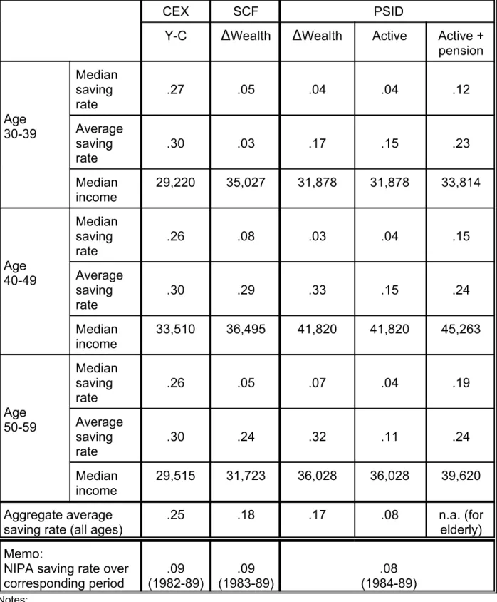
Table 2 shows summary measures of saving and income from the CEX, SCF, and PSID. All saving rates are on an annual basis, and all income figures are in 1989 dollars. To avoid undue influence from extreme values of the saving rate when income is close to zero, the “average” saving rates were calculated as average saving for the group divided by average income for the group.
The PSID “active” saving rates are generally the lowest in the table. By contrast, the estimates from the CEX — where saving is also based on the “active” concept — are among the highest. The high levels of CEX saving have been noted by previous authors (e.g. Bosworth, Burtless, and Sabelhaus, 1991) and probably reflect
measurement error: both income and consumption are understated by respondents but consumption is thought to be understated by a greater amount, lending an upward bias to saving.32 The PSID change in wealth (excluding pensions) saving measure, which includes capital gains and losses and adjusts for transfers in and out of the household, is generally higher than the PSID active saving measure and in the same ballpark as the similarly defined SCF measure.
We also calculate the saving rate averaged over the entire sample in each data set, including younger and older respondents, to correspond most closely to an
Table 2: Summary Saving and Income Measures
CEX SCF PSID
Y-C
)
Wealth)
Wealth Active Active + pensionAge 30-39
Median saving rate
.27 .05 .04 .04 .12
Average saving
rate .30 .03 .17 .15 .23
Median income
29,220 35,027 31,878 31,878 33,814
Age 40-49
Median saving rate
.26 .08 .03 .04 .15
Average saving rate
.30 .29 .33 .15 .24
Median income
33,510 36,495 41,820 41,820 45,263
Age 50-59
Median saving rate
.26 .05 .07 .04 .19
Average saving rate
.30 .24 .32 .11 .24
Median
income 29,515 31,723 36,028 36,028 39,620
Aggregate average saving rate (all ages)
.25 .18 .17 .08 n.a. (for
elderly) Memo:
NIPA saving rate over
corresponding period (1982-89).09 (1983-89).09 (1984-89).08
Notes:
1. The CEX figures correspond to after-tax income; the SCF figures correspond to pre-tax income; the PSID “change in wealth” and “active” figures correspond to after-tax income; the PSID “active+pension” figures correspond to the sum of after-tax income augmented by employer contributions to Social Security and pensions. All income data are expressed in 1989 dollars.
33 Note, though, that our saving measures include purchases of motor vehicles, which should
boost them relative to the NIPA concept.
34 Income quintiles were calculated (on a weighted basis for the SCF and PSID) for each age
group separately to ensure comparability across data sets and within the U.S. population. We did not use population weights in the regression analysis because the SCF weights — especially those for the top of the income distribution — ranged by orders of magnitude, causing considerable instability in the
estimated coefficients. For example, just three of the 107 households in the top 1 percent of the income distribution accounted for 38 percent of the total population weights among the replicated sample.
the final row -- conceptually, this rate is closest to the average “active” saving rate.33
V. Empirical Results
A. Saving Rates and Current Income
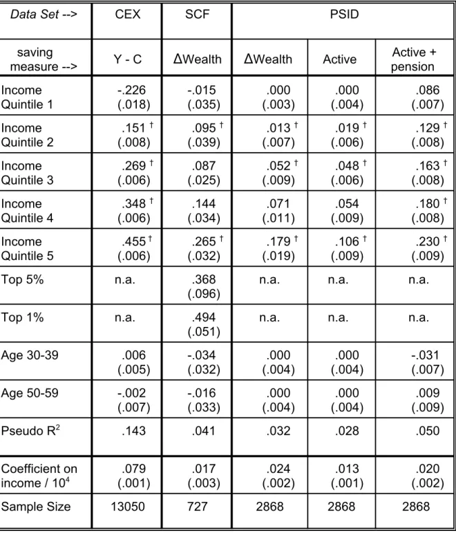
We begin our empirical inquiry by documenting the well-accepted fact that saving rates increase with current income. Table 3 summarizes how the saving rate varies with respect to current income quintile for households between the ages of 30 and 59.34 We estimate median regressions, with the saving rate as the dependent variable and dummies for income quintiles and age categories as independent variables. In each case, we suppress the constant term and include dummies for all five income quintiles and the 30-39 and 50-59 age groups so that the estimated coefficient for a given
income quintile corresponds to the saving rate for households in that quintile with heads between 40 and 49 years old. (Regressions that include interaction terms between age and income variables are similar.) Bootstrapped standard errors for the coefficients, based on 500 replications, are shown in parentheses.
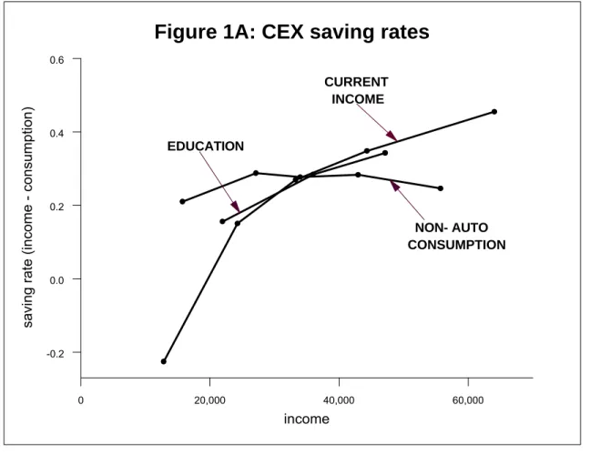
The first column of Table 3 shows that the saving rate increases dramatically with measured current income in the CEX. Among households with heads between 40 and 49, median saving rates range from -23 percent in the lowest income quintile to 46 percent in the highest. We also calculate (but do not report) bootstrapped standard errors for the difference in the saving rate of quintiles i and i-1, and use the symbol “ † ” to indicate a statistically significant difference, based on a 95% confidence level and a one-sided test. All of the differences in this column are statistically significant. To summarize the quintile effects, we also report the coefficient from a regression of saving rates on the level of income. This coefficient suggests that a $10,000 increase in income is associated with an 8 percentage point increase in the saving rate.
Table 3: Median Regressions of Saving Rate on Current Income
Data Set --> CEX SCF PSID
saving
measure --> Y - C
)
Wealth)
Wealth Active pension Active + Income Quintile 1 -.226 (.018) -.015 (.035) .000 (.003) .000 (.004) .086 (.007) Income Quintile 2.151 † (.008)
.095 † (.039)
.013 † (.007)
.019 † (.006)
.129 † (.008) Income
Quintile 3
.269 † (.006)
.087 (.025)
.052 † (.009)
.048 † (.006)
.163 † (.008) Income
Quintile 4 .348 †
(.006) (.034).144 (.011).071 (.009).054 .180 † (.008) Income
Quintile 5
.455 † (.006)
.265 † (.032)
.179 † (.019)
.106 † (.009)
.230 † (.009)
Top 5% n.a. .368
(.096)
n.a. n.a. n.a.
Top 1% n.a. .494
(.051)
n.a. n.a. n.a.
Age 30-39 .006
(.005) -.034(.032) (.004).000 (.004).000 -.031(.007) Age 50-59 -.002
(.007) -.016 (.033) .000 (.004) .000 (.004) .009 (.009)
Pseudo R2 .143 .041 .032 .028 .050
Coefficient on
income / 104 (.001).079 (.003).017 (.002).024 (.001).013 (.002).020
Sample Size 13050 727 2868 2868 2868
• Bootstrapped standard errors shown in parentheses.
• SCF and PSID quintiles are weighted; all regressions are unweighted.
• Definitions of income: CEX: current income; SCF: income in 1988; PSID: average income 1984-88.
35 We are able to estimate fairly precise saving rates for households in the highest part of the
income distribution because the SCF disproportionately samples high-income households – out of a total of 727 households in the age 30-59 sample, 201 have income above the 95th percentile and 107 have income above the 99th percentile.
36 The top quintile includes the top 5 percent, and the top 5 percent includes the top 1 percent.
We do not test whether the saving rates for the top 5 percent or the top 1 percent are different from the saving rates for the top quintile.
Consistent with previous research based on the CEX, we estimate an extremely low saving rate for the lowest income quintile; we believe this reflects appreciable bias from measurement error in income and/or transitory income, as households in this quintile presumably cannot sustain such a high rate of dissaving for very long (see Sabelhaus, 1993).
The second column shows results from similar regressions using SCF data, including (annualized) saving rate estimates for households in the 95th and 99th
percentile of the income distribution.35 The slope of the relationship between the saving rate and measured current income is smaller than in the CEX. This result is not
surprising – the change-in-wealth saving rate is not subject to the upward bias associated with measurement error in income, and many transitory movements in income likely wash out over the five-year period covered by the SCF panel. Nevertheless, we see the estimated median saving rate rising significantly from
-2 percent for households in the bottom quintile to 27 percent for households in the top quintile. Saving rates are even larger for the richest households: 37 percent for those in the top five percent of the income distribution and 49 percent for those in the top one percent.36
Columns 3 through 5 show the relationship in the PSID between income and three saving-rate measures: the (annualized) total change in wealth (Column 3), active saving (Column 4), and active saving plus imputed pension and Social Security saving (Column 5). As in the SCF, the five-year period over which saving is measured reduces the importance of transitory income (also note that we are able to average five annual observations for income). In all cases, we estimate a monotonic positive relationship between saving and income, with differences of as much as 18 percentage points between the highest and lowest income quintiles.
37 Among households aged 40-49 with any positive earnings, median Social Security saving as a
percent of pre-tax earnings ranges from 10.1 percent in the bottom income quintile to 4.2 percent in the top quintile. But when calculated as a percent of pre-tax earnings plus transfer income, median rates range from 8.2 percent in the bottom income quintile to 4.1 percent in the top quintile. (If we do not exclude the zero-earnings households, the latter range is 7.8 percent to 4.1 percent.)
38 For example, among households 40-49, median Social Security saving as a percentage of
disposable income ranges declines from 6.5 percent for the lowest income quintile to 3.9 percent for the highest income quintile. However, Social Security plus pension saving ranges rises from 7.6 percent in the lowest income quintile to 11.1 percent in the highest income quintile.
39 As mentioned previously, Gustman and Steinmeier (1997, tables 9 and 12, and 1999) use the
HRS to construct, for 51-61 year olds, a comprehensive measure of wealth that includes pension and Social Security wealth. They find that the ratio of the average comprehensive stock of wealth to average lifetime earnings declines with lifetime earnings; this is surprising in light of our results that ratios of saving flows with respect to income rise with income. In part, the difference can be explained by the fact that transfer income, an important source of income for low earnings households, is included in our income measure, but not included in theirs (see our footnote 37 above). Another reason may be that very long averages of lagged earnings could be imperfect measures of permanent income – as predictors of future earnings, these averages likely overweight the distant past. The finding in Gustman and Steinmeier (1997) that even the ratio of financial wealth to lifetime earnings does not increase with lifetime earnings deciles suggests mismeasurement of permanent income.
40 Moreover, Coronado, Fullerton, and Glass (1999), Liebman (1999), and Gustman and
Steinmeier (2000) show that Social Security is less progressive when the calculations are based on additional features not included in our model, such as life expectancies that are positively related to income.
Note that the differences in saving rates by income group for active saving augmented by imputed pension and Social Security contributions (Column 5) are even larger than those for active saving (Column 4). This may appear surprising, given the higher Social Security rates of return and replacement rates among households with lower earnings. There are two factors that explain this. First, while imputed Social Security saving rates as a percent of earnings are decreasing across income quintiles, when Social Security saving rates are calculated as a percent of earnings plus income transfers such as AFDC, disability and unemployment insurance, the decrease is somewhat smaller.37 Second, saving through private pensions increases across income quintiles, and this increase more than offsets the decline in Social Security saving, so that median Social Security plus pension saving is generally higher in the top quintile than in the bottom quintile.38 Thus it is unlikely that low rates of financial saving and wealth accumulation among lower income households can be explained by higher implicit Social Security and/or pension wealth accumulation.39,40
41 Because of non-linearities at very high levels of income, this regression excluded households
with income in excess of $500,000.
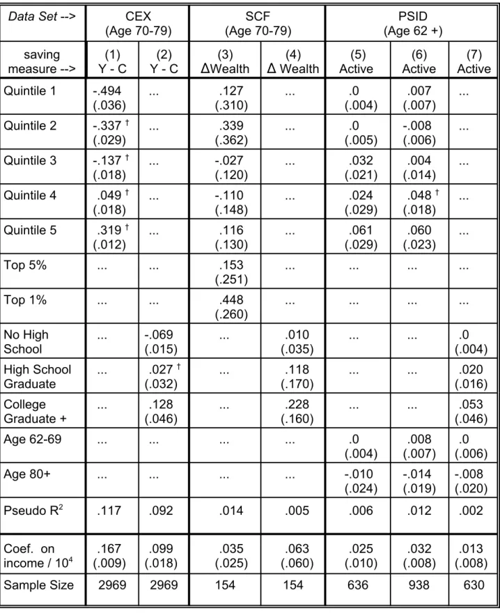
B. Saving Rates and Permanent Income
We now turn our attention to the relationship between saving rates and
permanent income, using the two-stage procedure described earlier. We first focus on consumption as an instrument. Recall that the presence of measurement error (in the case of the CEX) or transitory consumption (in all three data sets) will bias the
estimated slope toward a negative number.
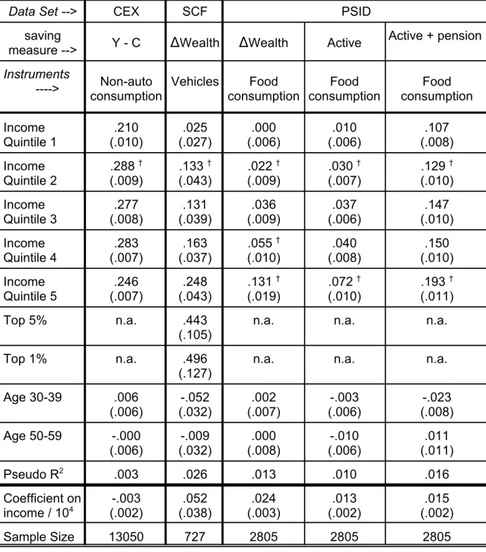
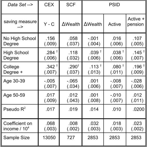
Column 1 of Table 4 shows results from the CEX. The estimated median saving rate rises from the predicted first to second quintile, but then remains fairly flat. One interpretation is that the results favor the Friedman proportionality hypothesis; the more likely is that the negative correlation induced by measurement error in consumption and transitory consumption is approximately offset by a positive correlation between saving rates and permanent income.
We next consider data from the SCF and PSID, where saving is derived from the change in wealth and is thus likely uncorrelated with consumption measurement error. The SCF does not contain direct consumption flow measures, but it does include estimates of the value of vehicle stocks. We use the value in 1983 as an instrument. As shown in column 2, the results based on this instrument are surprisingly similar to those in the previous table, with saving rates rising from 3 percent in the lowest quintile to 25 percent in the top quintile. Saving rates in the top 5 percent are 44 percent of income, and in the top 1 percent are nearly half of income. These results suggest that the positive relationship between saving rates and income is even stronger for the highest-income households. The estimated linear impact of income on saving rates (near the bottom of the table) is roughly 5 percentage points per $10,000 in income, but is not statistically significant.41
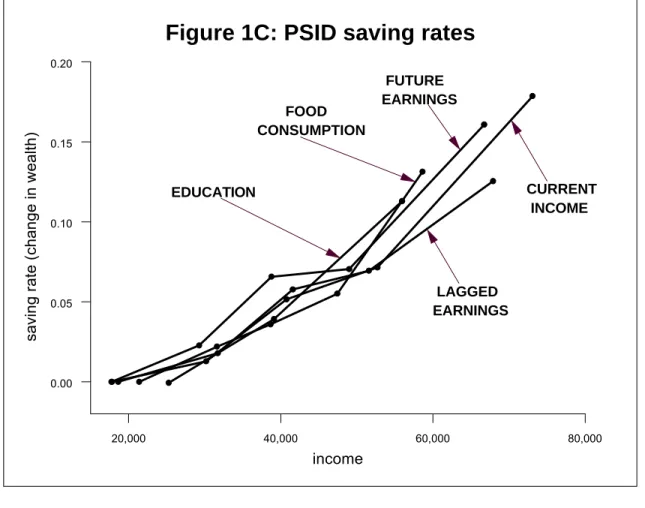
Although the PSID contains data on food consumption only, previous work using other data sets has generally shown a monotonic relationship between total
consumption and food consumption. Columns 3, 4, and 5 in Table 4 show that when PSID food consumption is used as an instrument, the estimated saving rates
Table 4: Median IV Regressions of Saving Rate on Income using Consumption as an Instrument
Data Set --> CEX SCF PSID
saving
measure --> Y - C
)
Wealth)
Wealth ActiveActive + pension
Instruments
----> consumptionNon-auto Vehicles consumptionFood consumptionFood consumptionFood
Income Quintile 1 .210 (.010) .025 (.027) .000 (.006) .010 (.006) .107 (.008) Income
Quintile 2 .288 † (.009) .133 † (.043) .022 † (.009) .030 † (.007) .129 † (.010) Income Quintile 3 .277 (.008) .131 (.039) .036 (.009) .037 (.006) .147 (.010) Income Quintile 4 .283 (.007) .163 (.037)
.055 † (.010) .040 (.008) .150 (.010) Income
Quintile 5 (.007).246 (.043).248 .131 † (.019) .072 † (.010) .193 † (.011)
Top 5% n.a. .443
(.105)
n.a. n.a. n.a.
Top 1% n.a. .496
(.127)
n.a. n.a. n.a.
Age 30-39 .006 (.006) -.052 (.032) .002 (.007) -.003 (.006) -.023 (.008) Age 50-59 -.000
(.006) (.032)-.009 (.008).000 (.006)-.010 (.011).011
Pseudo R2 .003 .026 .013 .010 .016
Coefficient on
income / 104 (.002)-.003 (.038).052 (.003).024 (.002).013 (.002).015
Sample Size 13050 727 2805 2805 2805
• Bootstrapped standard errors shown in parentheses.
• SCF and PSID quintiles are weighted; all regressions are unweighted.
42 In the first stage, we regress average current disposable income (1984-1988) on food
consumption in each of the years 1984-1987.
43 In fact, we had earnings information back to 1967, but, conditioning on earnings in more recent
years, those earlier readings had little or no predictive power for income in 1984-88.
consistently rise with income.42 Indeed, the saving rate shows a significant step-up for roughly half of the quintiles. The linear results at the bottom of the table are statistically significant and quantitatively important, pointing to a 1-1/4 to 2-1/2 percentage point increase in the saving rate for each $10,000 increment to predicted income.
Our next approach uses as instruments lagged and future earnings. For the CEX, we have no data on lagged or future earnings. For the SCF, we have only one observation on earnings from outside the measurement period for saving: 1982 income. Column 1 of Table 5 shows that when this variable is used as an instrument for 1988 income, there is a very strong relationship between predicted income and saving rates, with the very highest income groups saving half of their after-tax income. Only one of the differences is statistically significant, but the estimate from the linear equation (a 2 percentage point increase for each $10,000 in predicted income) is statistically
significant.
For the PSID, we use as instruments labor earnings of the head and wife (combined) for each year from 1974 to 1978, or effectively 10 years before the period over which saving is measured.43 Columns 2, 3, and 4 of Table 5 show the results of this approach for the three PSID saving measures. In all cases, saving rates rise with predicted permanent income. The magnitude of the differences are in fact quite close to those from the uninstrumented results in Table 3, suggesting that the simple five-year average of current income eliminated transitory income quite effectively.
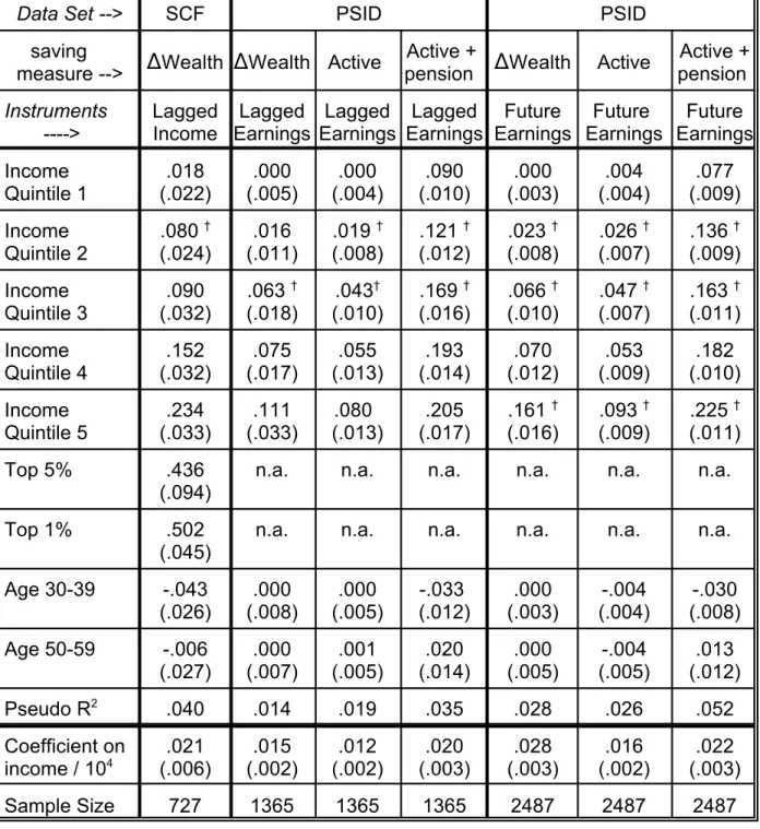
The last three columns of Table 5 show that when future earnings (1989-91) are used as instruments, we again see saving rates increasing with predicted income. This is true whether one looks at the quintile coefficients (ranging, for the active plus pension saving measure, from 8 percent to 23 percent) or the coefficient from the regression on predicted income (suggesting an increase of between 1-1/2 percentage points and 2-3/4 percentage points for each $10,000 increase in predicted income, with standard errors around 1/4 percentage point).
Table 5: Median IV Regressions of Saving Rate on Income using Lagged and/or Future Earnings as Instruments
Data Set --> SCF PSID PSID
saving
measure -->
)
Wealth)
Wealth ActiveActive +
pension
)
Wealth ActiveActive + pension Instruments ----> Lagged Income Lagged Earnings Lagged Earnings Lagged Earnings Future Earnings Future Earnings Future Earnings Income Quintile 1 .018 (.022) .000 (.005) .000 (.004) .090 (.010) .000 (.003) .004 (.004) .077 (.009) Income Quintile 2
.080 † (.024)
.016 (.011)
.019 † (.008)
.121 † (.012)
.023 † (.008)
.026 † (.007)
.136 † (.009) Income
Quintile 3 (.032).090 .063 † (.018) .043 † (.010) .169 † (.016) .066 † (.010) .047 † (.007) .163 † (.011) Income Quintile 4 .152 (.032) .075 (.017) .055 (.013) .193 (.014) .070 (.012) .053 (.009) .182 (.010) Income Quintile 5 .234 (.033) .111 (.033) .080 (.013) .205 (.017)
.161 † (.016)
.093 † (.009)
.225 † (.011)
Top 5% .436
(.094) n.a. n.a. n.a. n.a. n.a. n.a.
Top 1% .502
(.045)
n.a. n.a. n.a. n.a. n.a. n.a.
Age 30-39 -.043 (.026) .000 (.008) .000 (.005) -.033 (.012) .000 (.003) -.004 (.004) -.030 (.008) Age 50-59 -.006
(.027) .000 (.007) .001 (.005) .020 (.014) .000 (.005) -.004 (.005) .013 (.012)
Pseudo R2 .040 .014 .019 .035 .028 .026 .052
Coefficient on
income / 104 (.006).021 (.002).015 (.002).012 (.003).020 (.003).028 (.002).016 (.003).022
Sample Size 727 1365 1365 1365 2487 2487 2487
• Bootstrapped standard errors shown in parentheses.
• SCF and PSID quintiles are weighted; all regressions are unweighted..
• SCF results use 1988 income as current income and 1982 income as lagged income. • PSID results use 1974-1978 for lagged earnings and 1989-1991 for future earnings.