Numerical Analysis of Cyclically Loaded Concrete Under Large Tensile Strains by the Plastic-Damage Model

c

Sharif University of Technology, June 2010

Numerical Analysis of Cyclically

Loaded Concrete Under Large Tensile

Strains by the Plastic-Damage Model

O. Omidi

_{and V. Lot}

Abstract. Within the framework of plasticity-based constitutive laws, a plastic-damage model is developed in a complete form for analysis of damaged structures under large tensile strains which is suitable for concrete subjected to cyclic loadings. This is based on the plastic-damage model proposed by Lee and Fenves, which utilizes two separate damage variables for tension and compression and also a scalar degradation simulating damage on stiness. Implementation of the model is coded for three-dimensional space in a special purpose nite element program to analyze the behavior of concrete subjected to large tensile cracking, which is inevitable in plain concrete structures. In order to include large crack opening/closing displacements in the model, the excessive increase in plastic strain causing unrealistic results in cyclic behaviors is prevented when the tensile plastic-damage variable controlling the evolution of tensile damage is larger than a critical value. To expedite the convergence rate for the overall equilibrium iterations, the consistent algorithmic tangent stiness tensor is also derived, in detail, for large cracking states. The paper is completed with some numerical examples demonstrating the capability of the extended model in reproducing the behavior of cyclically loaded plain concrete subjected to large tensile strains. Keywords: Plastic-damage; Algorithmic tangent stiness; Large cracking; Nonlinear analysis; Stiness degradation.

INTRODUCTION

Constitutive theory of concrete materials has been one of the main themes of research for some decades. However, due to its composite nature, the complicated behavior of concrete cannot be satisfactorily reected in the usual constitutive theories of materials such as pure plasticity and pure damage mechanics theories, especially in cyclic loadings.

Continuum damage mechanics has been utilized extensively as a constitutive law of concrete [1-3]. Before the establishment of damage theories in the 1970s, the nonlinear response of concrete could only be captured using the plasticity theory, the nonlinear elasticity theory or the fracture theory [4-6]. Although these theories can solely yield adequate results that

1. Department of Civil and Environmental Engineering, Amirk-abir University of Technology, Tehran, P.O. Box 158754413, Iran.

*. Corresponding author. E-mail: [email protected]

Received 19 August 2009; received in revised form 18 January 2010; accepted 9 March 2010

match the corresponding experiments, in some cases, for example in monotonic loadings, it would be a better choice to combine these theories to obtain an appropri-ate constitutive model for concrete. The use of coupling between damage and plasticity has been found to be necessary for capturing the observed experimental-based behavior of concrete. Plastic-damage models have been developed and used by several researchers such as Yazdani and Schreyer [7], Lubliner et al. [8], Wu et al. [9], Jason et al. [10], Salari et al. [11], Lemaitre [12] and others [13-16].

A coupled damage-plasticity approach is, there-fore, adopted in this paper with emphasizing modica-tions to consider large tensile cracking states, which is vital for capturing appropriate results in plain concrete subjected to cyclic loadings [17,18]. Damage mechanics theory can model the strain softening and stiness degradation, while plasticity theory can capture the residual strains and some other macroscopic features. The behavior at the microscopic level is characterized by the damage indicators and plastic strains as the two representative macroscopic variables.

The nonlinear behavior of concrete is caused by three major sources of plasticity, cracking and time de-pendent eects such as creep, shrinkage, temperature, and load history. The plasticity behavior of concrete materials at the macroscopic level can be modeled by the classical plasticity theory [5]. On the other hand, the stiness degradation caused by the microcracking process, which can be observed in concrete structures subjected to cyclic loading, is dicult to be represented merely with the classical plasticity theory. However, in continuum damage mechanics, the degradation can be modeled by dening the relationship between stress and eective stress [2].

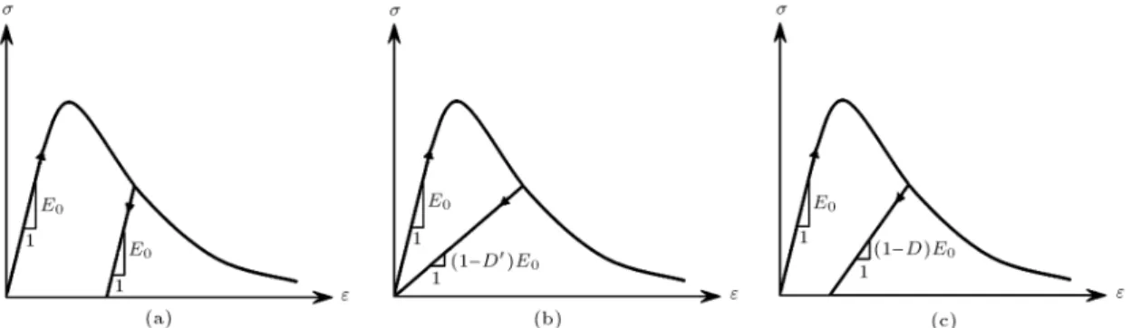
Therefore, one of the most important macroscopic features in constitutive modeling of concrete under cyclic loading is to capture the variations of the unload-ing stiness upon mechanical load reversal. Damage mechanics has the suitable theoretical background for this phenomenon but, since the concrete experiences also some irreversible deformations during loading, it cannot, alone, be implemented. As illustrated in Fig-ure 1, although plasticity and damage models are solely capable of representing the same material response during monotonic loading, both theories fail in cap-turing the evolution of unloading stiness accurately. In fact, in a pure damage approach, which is using secant unloading slope, it would result in an articial increase of damage due to neglecting plastic strains. In contrast to this phenomenon in a pure damage model, a pure plastic model employs an elastic modulus in unloading behavior because it cannot describe the damage eects during loading. Therefore, the coupled plastic and damage models are necessary in problems dealing with concrete structures under cyclic and/or dynamic loadings. Various coupled models have been proposed and used for analysis of concrete structures by many researchers in recent years [7-17].

In 1989, Lubliner et al. proposed a plastic-damage model which can be successfully applied for concrete under monotonic loading [8]. This model has a damage variable to represent both softening in tension and hardening in compression. It also uses elastic and

plas-tic degradation variables to simulate the degradation of elastic tangent, which is known to be very signicant in concrete. This model was modied by Lee and Fenves, in 1998, to include two damage variables; one in tension and another in compression [17,18]. This modication on Lubliner's model made it suitable to simulate the concrete under cyclic loading. Although Lee and Fenves proposed the model in 3-D and plane stress formulations, their implementation, examples and, nally, applications were limited to a 2-D plane stress state. In this study, the model implemented in 3-D space [19] is developed to consider large tensile cracking.

The proposed procedure for the stress update in large cracking states is implemented in a special nite element program, called SNACS [20]. The program solves the equations of motion incrementally using either load or displacement control.

The paper is organized as follows. Basic concepts of the constitutive relations of the plastic-damage model are presented in the next section for the usual cracking state. This section introduces the yield surface and the ow rule employed in the present study as well. The theoretical issues involved in large cracking states are discussed in the following section. The numerical integration aspects of the modied model are also ad-dressed in that section for large cracking states. After-wards, the procedure used for the stress update at each Gauss point, considering a large cracking eect, is high-lighted. The linearization of constitutive relations con-sistent with the stress computation algorithm in a large cracking state is derived in the next section. Finally, several numerical examples are presented to demon-strate the capability of the modied model, which is discussed and implemented in the present paper. PLASTIC-DAMAGE MODEL IN USUAL CRACKING STATE

The theoretical basics of the plastic-damage model are fully described in [17,18]. Reference [19] also presents the details of its numerical implementation in 3-D

space. Moreover, its main features are summarized in the following subsection.

Overview

In this subsection, the major components of the plastic-damage model are summarized. As a plasticity-based model, it begins with the strain decomposition as:

" = "e_{+ "}p_{; (1)}

in which " is the total strain, "e _{and "}p_{are the elastic}

part and the plastic part of the strain, respectively. Moreover, based on the scalar damage theory in com-bination with the plasticity theory, the stress-strain relation is written as:

= E : "e_{; (2a)}

E = (1 D)E0; (2b)

where is the stress tensor; E is the damaged elastic stiness tensor; E0 is the undamaged elastic

stiness tensor and D is the scalar stiness degradation variable, ranging from zero to one. Substituting the elastic part of the strain tensor from Equation 1 into Equation 2a, the stress-strain constitutive relation is constructed as:

= (1 D)E0: (" "p); (3)

in which the eective stress (i.e., = =(1 D)) would be as:

= E0: (" "p): (4)

It is noted that the plasticity part of the model is formulated in terms of the eective stress. Moreover, the evolution law for the plastic strain tensor, using a non-associative ow rule, is established as:

_"p_{= _r}

; (5)

where is the plastic potential function and is known as the consistency parameter. The yield function, which determines the yield state of stress, is written as:

F (; ) 0; (6)

where is a vector containing hardening variables that is referred to as normalized plastic-damage variables in this model. In plasticity-based models, hardening variables control the evolution of the yield surface. The damaged states in tension and compression are characterized independently by these plastic-damage variables, t and c. The plastic-damage vector is

dened as follows: =

t

c

: (7)

Corresponding to this plastic-damage vector, the degradation damage vector can be dened as:

D =

Dt(t)

Dc(c)

; (8)

in which, Dtand Dc are called tensile and compressive

damage variables, respectively. Each damage variable is dened as a function of its corresponding plastic-damage variable. The plastic-damage evolution equation is formed as:

_ = _H(; ): (9)

The mechanism of microcrack opening and closing behavior can be modeled as elastic recovery during elastic unloading from a tensile state to a compressive state. Since the model captures the two major damage phenomena, i.e. the uniaxial tensile and compressive ones, multi-dimensional degradation behavior can be possibly evaluated by interpolating between these two main damages, Dt and Dc, such as:

D = 1 (1 Dc)(1 sDt): (10)

The stiness recovery parameter denoted as s is con-sidered to simulate the elastic stiness recovery during the elastic unloading process from tensile state to compressive state, such that s0 s 1, considering

a minimum value of s0[17]:

s(^) = s0+ (1 s0)r(^); (11)

in which the scalar quantity, r(^), is a weight factor ranging from zero when all principal stresses are neg-ative, to one when they are all positive. Symbolizing hxi as the ramp function (i.e., hxi = (x + jxj)=2), r(^) is dened as:

r(^) =

3

P

i=1h^ii 3

P

i=1j^ij

: (12)

Moreover, r(^) = r(^), due to scalar degradation being applied to the elastic stiness tensor in the constitutive relation.

Plasticity Yield Surface

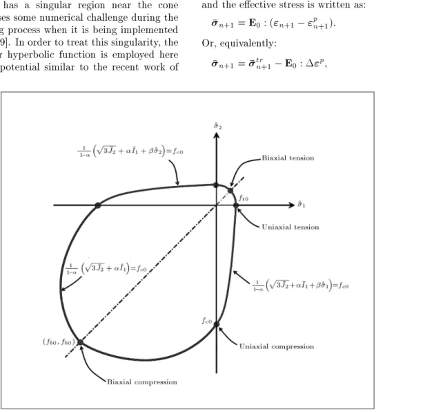
The constitutive law employs the yield surface of Lubliner in terms of the eective stress (not the stress), and the plastic-damage variables as:

F (; ) = f(; ) cc(); (13a)

f(; ) =₁ 1 "

p

3 J2+ I1

+ ()h^maxi h ^maxi

#

in which and have the following denitions: = (fb0=fc0) 1

2(fb0=fc0) 1; (14)

= c_cc(c)

t(t)(1 ) (1 + ): (15)

Here, fb0=fc0 is the ratio of the initial yield strengths

under equibiaxial and uniaxial compression; ct and

cc are the tensile and compressive cohesions. The

parameter appears only in triaxial compression with ^max< 0 and, usually, is equal to 3 [8]. It is noted that

the yield surface can be represented equivalently by an alternative form as F (; ) = ^F (^; ) [18]. It is also illustrated in Figure 2 for the plane stress space. Plasticity Flow Rule

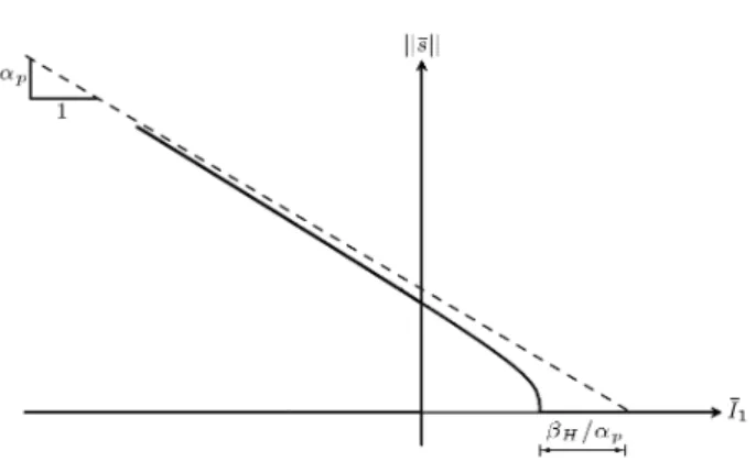
In the original formulation proposed by Lee and Fenves [17], the Drucker-Prager linear function was used and implemented for the plane stress problem. This function has a singular region near the cone tip, which causes some numerical challenge during the return-mapping process when it is being implemented in 3-D space [19]. In order to treat this singularity, the Drucker-Prager hyperbolic function is employed here as the plastic potential similar to the recent work of

Saritas and Flilippou [21]. This function is expressed in terms of the eective stresses, as below, and also depicted in the meridian plane in Figure 3. Being continuous and smooth, it causes the ow direction to be always uniquely dened.

() =q2

H+ 2 J2+ pI1: (16)

Here, H would be:

H = "1pft0; (17)

and parameter p should be calibrated to give proper

dilatancy [17]. Stress Integration

The stress integration algorithm consists of an elastic predictor, plastic and damage correctors. From Equa-tion 3, at time step n + 1, the stress is formed as:

n+1= (1 Dn+1)n+1; (18)

and the eective stress is written as:

n+1= E0: ("n+1 "pn+1): (19)

Or, equivalently:

n+1= trn+1 E0: "p; (20)

Figure 3. Schematic representation of the Drucker-Prager hyperbolic function.

where tr

n+1 plays the role of the elastic predictor and

is called trial eective stress: tr

n+1= E0: ("n+1 "pn): (21)

When the trial eective stress state is out of the current yield surface (i.e., F (tr

n+1; n) > 0), the plastic strain

and also damage variables will change. In the plastic corrector part, the eective stress and plastic-damage variables are updated using linearization of the damage evolution equation, whose discrete version is written as below by the backward-Euler method:

= H(^n+1; n+1): (22)

Or, equivalently:

n+1= n+ H(^n+1; n+1); (23)

in which is used instead of for simplicity. Since Equation 23 is a nonlinear function of , a residual denoted by Q (Equation 24) is dened and an iterative solution scheme for computing ^n+1, n+1and needs

to be established.

Q(^n+1; n+1; )= n+1+n+H(^n+1; n+1):

(24) In fact, this iteration procedure, which is referred to as the local iteration, imposes the following constraint to the return-mapping process.

Q(^n+1; n+1; ) = 0: (25)

Equation 25 is iterated using the Newton-Raphson scheme as:

dQ

d (j)

n+1 = Q (j)

n+1; (26)

where dQ=d is the Jacobian matrix of Q, with respect to , and is used to update the plastic-damage variables vector, n+1:

(j+1)_n+1 = (j)_n+1+ : (27)

Another constraint to the return-mapping process is the discrete version of the plastic consistency condi-tion, Equation 28, which is utilized to compute the consistency parameter, :

^

F (^n+1; n+1) = 0: (28)

It is noted that the spectral return-mapping algorithm is employed here, based on spectral decomposition of the eective stress. It is well-known that spectral mapping is more ecient than general return-mapping when the yield surface includes principal ef-fective stress in addition to its invariants. The eective stress, as a symmetric matrix, can be factorized by the spectral decomposition:

n+1= Pn+1^n+1PTn+1; (29)

in which Pn+1 and ^n+1 are the non-singular matrix,

whose columns are the orthonormal eigenvectors of n+1and the diagonal matrix of eigenvalues of n+1,

respectively. As proved in [18], any eigenvector matrix of n+1is also an eigenvector matrix of trn+1, i.e.:

tr

n+1= Pn+1^trn+1PTn+1: (30)

Moreover, since an isotropic material behavior is as-sumed, there exists a function ^, such that ^(^) = (). Thus, the plastic strain increment can also be written in the spectral decomposition form [22]:

"p_{= P}

n+1r^^PTn+1: (31)

In fact, the eigenvalue matrix for the plastic strain increment becomes:

^"p= r^^: (32)

By using the Drucker-Prager hyperbolic plastic func-tion introduced in Equafunc-tion 16, ^"p yields:

^"p= 0

@_q ^sn+1

2

H+^sn+12

+ pI

1

A ; (33)

where ^sn+1 is the deviatoric part of the principal

eective stresses,^n+1.

PLASTIC-DAMAGE MODEL IN LARGE CRACKING STATE

The extension of the model for large crack opening and closing is discussed in this section. It should be noted that the basic idea for the large cracking modication has been initially presented in [23]. However, its formulation and 3-D implementation are emphasized in a complete manner in this paper, including the details of the stress update algorithm. Moreover, it is worthwhile to mention that the consistent algorithmic tangent stiness is also derived for large cracking states herein, something that is not discussed in the original studies of Lee and Fenves [23].

Large Cracking Modication

To simulate a large crack opening, closing and reopen-ing process in such a continuum model, the evolution law used for the damage variables needs to be modied. Actually, after a large amount of microcracking, the crack opening and closing mechanism becomes similar to discrete cracking. Here, it is assumed that the microcracks are joined to construct a discrete large crack, if t cr, where cr is a critical value for

the tensile damage. At such a tensile damage level, evolution of the plastic strain caused by the tensile damage is stopped and the plastic strain rate is dened as:

_"p= (1 r)_~"p_{; (34)}

_~"p_{= _r} ~

(~); (35)

in which ~"p _{is an intermediate plastic strain and r is a}

weight function, which could be possibly dened as:

r = r(^~); (36)

and ~ is an intermediate eective stress, which is dened as below:

~ = E0: (" ~"p) 2 f~jF (~; ) 0g : (37)

In order to make the eective stress based on the intermediate plastic strain admissible in the stress space, it is necessary to introduce a new degradation variable denoted by Dcr, and modify the eective stress

as:

mod= (1 Dcr)E0: (" "p): (38)

The new degradation damage variable, Dcr, is

de-termined by the following Kuhn-Tucker type load-ing/unloading conditions such that:

_Dcr 0; F ((1 Dcr); ) 0;

_DcrF ((1 Dcr); ) = 0; (39)

where F is the yield function. During plastic loading, the condition of F ((1 Dcr); ) = 0 leads to:

Dcr= 1 _{f(; )}cc() : (40)

The stiness degradation variable is redened to in-clude the new large-cracking degradation variable as:

D = 1 (1 Dc)(1 sDt)(1 sDcr): (41)

Numerical Implementation

In order to numerically implement the large cracking formulation described in the previous section, a three-step return-mapping algorithm is used here. First, the trial eective stress (as the elastic predictor step) is computed by Equation 38. Similar to the tensile damage variable, Dcr

n also needs to be multiplied

by the stiness recovery parameter, s, to capture the correct crack opening/closing behavior during the elastic unloading process from tension to compression and vice versa. The trial eective stress is modied as below:

~tr_n+1= (1 str

n+1Dncr)trn+1; (42)

where str

n+1, is computed based on the trial eective

stress: str

n+1= s(^trn+1): (43)

The trial eective stress is admissible as the eective stress at the current time step if:

F (~tr_n+1; n) = f(~trn+1; n) cc(n) 0: (44)

Otherwise, the plastic corrector is required to make the eective stress admissible. At the plastic corrector step, an increment of the intermediate plastic strain is integrated using the backward-Euler method:

~"p₌ @

@~n+1: (45)

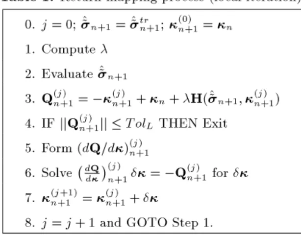
The return-mapping process is embedded in the local iteration mentioned above and is presented in Table 1. It should be noted that the stress which is being modied and mapped to the yield surface in the local iteration scheme is the intermediate eective stress, ~, not the true eective stress, which is denoted by .

After computing ~"p _{from the return-mapping}

scheme, the plastic strain is updated by: "p_n+1= "p

n+ (1 rn+1)~"p; (46)

Table 1. Return-mapping process (local iteration). 0. j = 0; ^~n+1= ^~trn+1; (0)n+1= n

1. Compute 2. Evaluate ^~n+1

3. Q(j)

n+1= (j)n+1+ n+ H(^~n+1; (j)n+1)

4. IF jjQ(j)

n+1jj T olLTHEN Exit

5. Form (dQ=d)(j)n+1

6. Solve dQ d

(j)

n+1 = Q (j) n+1 for

7. (j+1)

n+1 = (j)n+1+

where rn+1 is computed if tn+1 cr or otherwise

equals to zero. At the next step, the crack damage corrector causes the evaluated eective stress to return back onto the yield surface:

Dcr

n+1= 1 _f(cc(n+1)

n+1; n+1); (47)

in which n+1 is computed by Equation 20. Finally,

for the damage corrector step, the stress is computed by computing the degradation variable, Dn+1 as the

following: Dn+1= 1

(1 Dc

n+1)(1 sn+1Dtn+1)(1 sn+1Dcrn+1); (48)

where:

sn+1= s(^n+1): (49)

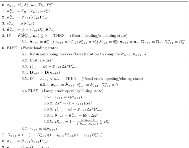
STRESS UPDATE ALGORITHM

The stress computation procedure is summarized in this section considering the possibility of large crack

opening/closing states. As mentioned above, the spectral return-mapping, which has some advantages with respect to general return-mapping, is being uti-lized here to decouple the return-mapping algorithm. The procedure begins with the spectral decomposition of the trial eective stress. In this approach, the principal stresses which play an important role in the model are computed in an ecient and explicit way. Moreover, its decoupled nature signicantly simplies the stress updating formulation. Table 2 summarizes the employed algorithm directly connected to the implementation of the model in a special nite element code [20]. At each step, the total strain is prescribed to each Gauss point and then the corresponding stress and other needed variables are updated by using the governing constitutive equations and loading-unloading conditions.

ALGORITHMIC TANGENT STIFFNESS IN LARGE CRACKING STATE

The iterative solution procedure in Newton's method requires the tangent stiness as a numerical technique for solving the nonlinear equilibrium equations.

Uti-Table 2. Stress update algorithm considering large tensile cracking. 0. "n+1, "pn, ~"pn, n, Dn, Dncr

1. tr

n+1= E0 : ("n+1 "pn)

2. tr

n+1= Pn+1^trn+1PTn+1

3. str

n+1= s(^trn+1)

4. ^~tr

n+1= (1 strn+1Dcrn)^trn+1

5. IF F (^~^ tr

n+1; n) 0 THEN (Elastic loading/unloading state)

5.1. ^n+1= ^trn+1; sn+1= strn+1; "pn+1= "pn; ~"n+1p = ~"pn; n+1= n; Dn+1= Dn; Dn+1cr = Dcrn

6. ELSE (Platic loading state)

6.1. Return-mapping process (local iteration to compute ^~n+1, n+1, )

6.2. Evaluate ^~"p

6.3. ~"p

n+1= ~"pn+ Pn+1^~"pPTn+1

6.4. Dn+1= D(n+1)

6.5. IF t

n+1< cr THEN (Usual crack opening/closing state)

6.5.1. ^n+1= ^~n+1; "pn+1= ~"pn+1; Dcrn+1= 0

6.6 ELSE (Large crack opening/closing state) 6.6.1. rn+1= r(^~n+1)

6.6.2. ^"p_{= (1 r}

n+1)^~"p

6.6.3. "p

n+1= "pn+ Pn+1^"pPTn+1

6.6.4. ^n+1= ^trn+1 E0: ^"p

6.6.5. Dcr

n+1= 1 _f(^^cc_n+1(n+1_;n+1) ₎ Dcrn

6.7. sn+1= s(^n+1)

7. Dn+1= 1 (1 Dcn+1)(1 sn+1Dn+1t )(1 sn+1Dcrn+1)

8. n+1= Pn+1^n+1PTn+1

lizing the algorithmic tangent stiness in the global iteration algorithm accelerates the convergence rate in comparison with employing the continuum tangent stiness [18], and it is consistent with the local iteration being used as the return-mapping process. After the converged eective stresses, damage variables and plastic strains are computed for the given strain; all the residual equations are assumed to be satised. In the following, the algorithmic tangent stiness is derived in the large cracking state (i.e., t

n+1 cr). This begins

by taking the total dierential of computed stress at the current time step:

d = n+1dD + (1 Dn+1)d; (50)

in which dD and d are derived as follows. From Equation 19:

d = E0: (d" d"p): (51)

Substituting d"p _{= (1 r}

n+1)d~"p from Equation 46

into the dierential of the eective stress, Equation 51, results in:

d = E0: [d" (1 rn+1)d~"p]: (52)

One can rearrange Equation 52 such that the dieren-tial intermediate eective stress appears in the relation as the following:

d = rn+1E0: d" + (1 rn+1)E0: (d" d~"p): (53)

Furthermore, the dierential of the intermediate eec-tive stress becomes:

d~ = E0: (d" d~"p): (54)

Utilizing Equation 54 causes Equation 53 to be rewrit-ten as:

d = rn+1E0: d" + (1 rn+1)d~: (55)

The total dierential of the degradation (i.e., Dn+1(Dn+1; Dcrn+1^n+1), which is computed in terms

of Dn+1(n+1), Dn+1cr (n+1; ^n+1) and ^n+1, may be

written as: dD = @D

@D: @D @:d +

@D @Dcr @Dcr @ :d + @D @Dcr @Dcr @^ : @^ @ : d +

@D @^ :

@^

@ : d: (56) Or, in a rearranged form as:

dD = @D @D: @D @ + @D @Dcr @Dcr @ :d + @D @^ + @D @Dcr @Dcr @^

: @^_@ : d; (57)

where the tensor @^=@ , which is a function of the general stress, is called the Jacobian tensor of the principal eective stress.

During the local iteration for obtaining the up-dated vector of the plastic-damage variables, the change of the residual vector is expected to be zero, i.e. dQ = 0:

@Q @:d +

@Q @^~ : d^~ +

@Q

@d = 0: (58)

By rearranging the above equation, the dierential of the plastic-damage vector becomes:

d = T~: d~ + Td; (59)

in which T~ and T are dened as below:

T~=

_@Q @ 1 :@Q @^~ : @^~

@ ~; (60)

T=

@Q @

₁

:@Q_@: (61)

Substituting Equation 59 into Equation 57, dD would be:

dD = TI

D ~: d~ + TIID : d + TDd; (62)

where TI

D ~, TIID and TD will have the following

denitions: TI

D ~=

@D @D: @D @ + @D @Dcr @Dcr @

:T~; (63)

TII D =

@D @^ + @D @Dcr @Dcr @^

: @^_@ ; (64)

TD=

@D @D: @D @ + @D @Dcr @Dcr @

:T: (65)

Substitution of Equation 55 into Equation 62 leads to: dD = TI

D ~: d~

+ TII

D : [rn+1E0: d" + (1 rn+1)d~]

+ TDd: (66)

Similarly, the total dierential of the yield function gives:

r_^~F : d^~ + r^ F :d = 0:^ (67)

By substituting Equation 59 into Equation 67, it is reformulated as:

where T_{F ~}^ and T_F ^ represent the following parts:

T_{F ~}^= r^~F :^ _{@ ~}@^~+ rF :T^ ~; (69)

T_F ^ = rF :T^ ; (70)

in which the total dierential of the intermediate plastic strain increment is:

d~"p= r~d + @ 2

@~2 : d~: (71)

By dening a pseudo-elastic stiness tensor as: S =

E 1

0 + @ 2

@~2

1

: (72)

Equation 54 is rewritten as the following form:

d~ = S : d" S : r~d: (73)

Substituting Equation 73 into Equation 68, d be-comes:

d =

T_F ^ : S

T_{F ~}^: S : r~ T_F ^

: d": (74) Finally, substitution of Equation 55 and Equation 66 into Equation 50 leads to the consistent algorithmic tangent stiness for large cracking states:

@ @"

n+1=rn+1

(1 Dn+1)I n+1TIID

: E0

+(1 Dn+1)(1 rn+1)I

n+1 TID ~+ (1 rn+1)TIID

: @ ~

@"

TDn+1@_@"; (75)

in which, from Equation 73 and Equation 74 the following equations are obtained:

@ ~ @" = S

S : r~ TF ~^ : S

T_{F ~}^ : S : r~ T_F ^ ; (76)

@ @" =

TF ~^: S

T_{F ~}^: S : r~ T_F ^ : (77)

In the usual cracking state (i.e., t

n+1< cr), one can

set rn+1 = 0 and, therefore, n+1 = ~n+1, which

leads to TD = TID + TIID . In such a condition,

the consistent algorithmic tangent stiness in the usual cracking state could be concluded from Equation 75 as:

@

@"

n+1

= [(1 Dn+1)I n+1 TD ] : @ _@"

TDn+1@_@": (78)

It should be noted that due to employing a non-associative ow rule and the existence of the degra-dation component, the algorithmic tangent stiness derived for both usual and large cracking states (i.e., Equations 75 and 78) is not symmetric [18].

NUMERICAL EXPERIMENTATION

The developed plastic-damage model implemented based on the algorithm discussed above is examined in this section. This is performed by means of several validations carried out by a displacement control ap-proach. Moreover, 8-node isoparametric solid elements with a 222 Gauss integration scheme are used in all examples. As is common [8,17,24], exponential forms are used here for softening parts of both tension and compression curves.

One-Element Tests

A single-element mesh is subjected to monotonic and cyclic loading, both in tension and compression. The responses are compared with the experimental results available in the literature. Table 3 shows the material properties utilized for all cases, unless otherwise speci-ed.

In this table, f0

t and fc0 are the maximum

uni-axial tensile and compressive strengths, respectively. Furthermore, the fracture energy in tension and the counterpart of fracture energy in compression are denoted by Gtand Gc, respectively.

The rst two tests discussed here conrm the basic capabilities of the model in the simulation of concrete under monotonic tensile and compressive load-ings. The responses to these fundamental loadings are evaluated and compared with the corresponding experiments and results from Lee and Fenves. It needs to be mentioned that in the uniaxial compressive case, elastic modulus, E0 of 31.7 GPa is utilized instead

of 31.0 GPa. Figure 4 depicts the simulated tensile and compressive stress-strain curves, respectively. As compared, the numerical results agree well with the experimental data [25,26] and also with the solutions of Lee and Fenves [17].

Subsequently, cyclic loading is applied to examine the capability of the model in capturing stiness degra-dation in both tensile and compressive loadings. The material properties are the same as those of Table 3, except E0 = 31:7 GPa. Figures 5a and 5b illustrate

the numerical results from two uniaxial cyclic loading cases compared with the experiments.

In another single-element test, cyclic loading un-der large tensile strains is imposed as the tension-compression-tension load. The results are compared in Figure 6 for both cases of with and without the possibility of a large crack opening/closing. As

ob-Figure 4. Monotonic uniaxial loadings compared with experiments [25,26] and also with Lee and Fenves's results [17].

Figure 5. Cyclic loading results in comparison with experiments [25,26].

Table 3. Material properties for the tests carried out. E0

(GPa) {

f0 t

(MPa) f0

c

(MPa) Gt

(N/m)

Gc

(N/m) {

p

{

lch

(mm) s0

{

31.0 0.18 3.48 27.6 12.3 1750.0 0.12 0.2 25.4 0.0

served, after a certain point, a continuum discrete crack is formed and the crack is closed afterwards during unloading from tension to compression. This example well conrms the necessity of considering the possibility of large crack opening/closing states in plain concrete under high tensile strains.

In the last case, the single element is subjected to full cyclic loading (Figure 7). This perfectly illustrates the ability of the model to simulate stiness recovery when the status changes from tension to compression and vice versa. This case also shows that if a large cracking option is not included in the stress update algorithm, it could lead to unrealistic results, as illus-trated in Figure 7 for the case in which cr is equal

to 1.0.

Structural Applications Mesh Sensitivity Test

The sensitivity to mesh size has been analyzed to check the mesh-objectivity, which is expected to be obtained by using the mesh-dependent characteristic length [8,17]. The geometry of the specimen, its boundary conditions and the meshes employed are illustrated in Figure 8. The utilized material properties are: E0 = 30 GPa, = 0:2, ft0 = 3:3 MPa, Gt =

1000 N/m, p = 0:2. In each case, the characteristic

length equals the mesh size in the horizontal direction.

Figure 7. Full cyclic loading results in dierent critical damage levels.

Figure 8. Mesh sensitivity analysis: (a) Geometry and boundary conditions of the specimen; (b, c and d) 3-D 8-node nite element meshes.

To make the strain localization occur at the left-end element consistently, the perturbation using less tensile strength was imposed on that element.

The resulting load-displacement curves are shown in Figure 9 for the dierent meshes including unloading and reloading. As observed, it is clear that since the ratio of the softening bandwidth to the length of the elastic unloading zone is dierent in each case, one cannot expect to have identical load-displacement responses, for either the loading or unloading parts. Nevertheless, the global loading or unloading responses become similar to each other (i.e., mesh objectivity is preserved), as the softening bandwidth becomes

Figure 9. Load-deection curves with unloading in dierent meshes.

smaller. Obviously, one expects a better match with experimental data as ner meshes are utilized.

In the following, the mesh MST3 is subjected to a large tensile strain and it is unloaded subsequently to check the algorithm in a large cracking state. The response considering large cracking is compared with the case of usual cracking in Figure 10a. As discussed before, at a specic tensile damage level, cr, the

evolution of plastic strain caused by the tensile damage is stopped and the microcracks are joined to form a discrete crack, if t cr (Figure 10b).

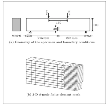
Four-Point Bending Test Under Cyclic Loading

Experimental results of notched beams have been widely employed to validate the corresponding numerical simulations captured by a proposed model [8,16,18,27]. In order to examine the plastic-damage model under cyclic loadings in a real applica-tion, the analysis of a notched concrete beam under four-point bending is investigated here. This example, which was experimentally performed by Horidijk in 1991 [28], is simulated using 3-D modeling. The specication of the specimen and the three-dimensional

Figure 10. (a) Comparison of load-deection curves for usual and large cracking (b) plastic strain ("p

x) vs

intermediate plastic strain (~"p

x) in the case of cr= 0:95.

8-node nite element mesh of a half-beam model are depicted in Figure 11.

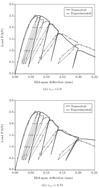
The material properties used in this application are as listed in Table 4. In this test, cr of 0.75 is

used to include the large cracking phenomenon. Fig-ure 12 shows the load P versus the mid-span deection for the numerical simulation and the corresponding experimental test. The results closely agree with the experiment, indicating the good accuracy of the solution during unloading and reloading.

The state of tensile damage along with the dis-placed shape at the end of the analysis is also illustrated in Figure 13 for each case. Comparison of the damage patterns for the two cases shows that the modication needed for considering large cracking slightly aects the damage evolution process.

CONCLUSIONS

Development of a plastic-damage model to capture the proper cyclic behavior of concrete under large tensile strains is presented in a complete manner. The algorithmic tangent stiness, which is consistent with the stress update algorithm, is derived in detail for the large cracking state. The plastic-damage model, which is implemented for 3-D space in this study, was initially proposed by Lee and Fenves, in 1998. Although

Figure 11. Four-point bending test. Table 4. Material properties for the four-point bending test.

E0

(GPa) {

f0 t

(MPa) f0

c

(MPa) Gt

(N/m) Gc

(N/m)

{ p

{ s0

{

Figure 12. Four-point bending test, load-deection curve compared with the experiment [28].

the damage part of the model is isotropic, it utilizes two damage variables, one in tension and another for compression, which makes it suitable for cyclic responses. Moreover, the return-mapping process eciently employs the spectral decomposition form of the stress matrix.

Although damage and plasticity theories sepa-rately are capable of capturing the same material response upon monotonic loading, neither model sim-ulates the evolution of unloading stiness accurately. Neglecting plastic strains in a pure damage approach would result in an articial increase of damage as the secant unloading slope. Hence, a coupled damage-plasticity model could be a solution, but it also fails to properly model the cyclic-loaded concrete under large tensile strains, because, after joining microc-racks, a discrete crack is formed and, subsequently,

Figure 13. Tensile damage pattern along with the displaced shape at the end of the analysis.

usual cracking no longer works. In large crack-ing states, evolution of the tensile plastic strain is stopped. In this condition, the evolution law used for the damage variables needs to be modied. In fact, after a large amount of microcracking, if the tensile damage is more than a critical value, the crack opening/closing mechanism becomes similar to discrete cracking.

Through single-element tests, the implemented algorithm is shown to give numerical simulations that work appropriately. It is also conrmed that the modications discussed should be applied to the model in the problems experiencing large tensile strains under cyclic loading. At the end, a single-notched beam under four-point bending is investigated numerically. It is also compared with the corresponding experimental results. Comparison of the cases analyzed demon-strates that including the large crack opening/closing prevents excessive tensile plastic strains causing unre-alistic results. Furthermore, the necessity of such a modication is emphasized to properly simulate the cyclic behavior of plain concrete under large tensile strains.

REFERENCES

1. Loland, K.E. \Continuous damage model for load-response estimation of concrete", Cement & Concrete Research, 10, pp. 395-402 (1980).

2. Mazars, J. and Pijaudier-Cabot, G. \Continuum dam-age theory: Application to concrete", Journal of Eng. Mechanics, 115, pp. 345-365 (1989).

3. Lubarda, V.A., Kracjinvovic, D. and Mastilovic, S. \Damage model for brittle elastic solids with unequal

tensile and compressive strength", Engineering Frac-ture Mechanics, 49, pp. 681-697 (1994).

4. William, K.J. and Warnke, E.P. \Constitutive model for the triaxial behavior of concrete", Int. Association of Bridge and Structural Engineers, Seminar on Con-crete Structure Subjected to Triaxial Stresses, Paper III-1, Bergamo, Italy (1975).

5. Menetrey, Ph. and Willam, K.J. \Triaxial failure criterion for concrete and its generalization", ACI Structural Journal, 92, pp. 311-318 (1995).

6. Grassl, P., Lundgren, K. and Gylltoft, K. \Concrete in compression: a plasticity theory with a novel hardening law", Int. J. of Solids and Structures, 39, pp. 5205-5223 (2002).

7. Yazdani, S. and Schreyer, H.L. \Combined plasticity and damage mechanics model for plain concrete", Journal of the Engineering Mechanics Division, ASCE, 116, pp. 1435-1450 (1990).

8. Lubliner, J., Oliver, J., Oller, S. and Onate, E. \A plastic-damage model for concrete", Int. J. of Solids Structures, 25, pp. 299-326 (1989).

9. Wu, J.U., Li, J. and Faria, R. \An energy release rate-based plastic-damage model for concrete", Int. J. of Solids and Structures, 43, pp. 583-612 (2006). 10. Jason, L., Huuerta, A., Pijaudier-Cabot, G.,

Ghavamian, S. \An elasto plastic damage formulation for concrete: Application to elementary tests and com-parison with an isotropic damage model", Computer Methods in Applied Mechanics and Engineering, 195, pp. 7077-7092 (2006).

11. Salari, M.R., Saeb, S., Willam, K.J., Patchet, S.J. and Carrasco, R.C. \A coupled elastoplastic damage model for geomaterials", Computer Methods in Applied Me-chanics and Engineering, 193, pp. 2625-2643 (2004). 12. Lemaitre, J. \Coupled elasto-plasticity and damage

constitutive equations", Computer Methods in Applied Mechanics and Engineering, 51, pp. 31-49 (1985). 13. Gatuingt, F. and Pijaudier-Cabot, G. \Coupled

dam-age and plasticity modeling in transient dynamic anal-ysis of concrete", Int. J. of Numerical and Analytical Methods in Geomechanics, 26, pp. 1-24 (2002). 14. Menzel, A., Ekh, M., Runesson, K. and Steinmann, P.

\A framework for multiplicative elastoplasticity with kinematic hardening coupled to anisotropic damage", Int. J. of Plasticity, 21(3), pp. 397-434 (2005). 15. Abu Al-Rub, R.K. and Voyiadjis, G.Z. \On the

cou-pling of anisotropic damage and plasticity models for ductile materials", Int. Journal of Solids and Struc-tures, 40, pp. 2611-2643 (2003).

16. Nguyen, G.D. and Korsunsky, A.M. \Development of an approach to constitutive modeling of concrete: isotropic damage coupled with plasticity", Int. J. of Solids and Structures, 45, pp. 5483-5501 (2008). 17. Lee, J. and Fenves, G.L. \A plastic-damage model for

cyclic loading of concrete structures", J. of Engineer-ing Mechanics, ASCE, 124, pp. 892-900 (1998).

18. Lee, J. and Fenves, G.L. \A return-mapping algorithm for plastic-damage models: 3-D and plane stress formu-lation", Int. J. for Numerical Methods in Engineering, 50, pp. 487-506 (2001).

19. Omidi, O. and Lot, V. \Finite element analysis of concrete structures using plastic-damage model in 3-D implementation", Submitted to Int. Journal of Civil Engineering (2010).

20. Omidi, O., SNACS: A program for Seismic Nonlinear Analysis of Concrete Structures, Department of Civil and Environmental Engineering, Amirkabir University of Technology, Tehran, Iran (2010).

21. Saritas, A. and Filippou, F.C. \Numerical integration of a class of 3-D plastic-damage concrete models and condensation of 3-D stress-strain relations for use in beam nite elements", Engineering Structures, 31(10), pp. 2327-2336 (2009).

22. Simo, J.C. \Algorithm for static and dynamics multi-plicative plasticity that preserve the classical return-mapping schemes of the innitesimal theory", Com-puter Methods in Applied Mechanics and Engineering, 99, pp. 61-112 (1992).

23. Lee, J. and Fenves, G.L. \A plastic-damage model for earthquake analysis of dams", Earthquake Engineering and Structural Dynamics, 27, pp. 937-956 (1998). 24. Mod, M. and Khezrzadeh, H. \Interpretation of

tensile softening in concrete using fractal geometry", Scientia Iranica, 15(1), pp. 8-15 (2008).

25. Gopalaratnam, V.S. and Shah, S.P. \Softening re-sponse of plain concrete in direct tension", ACI Jour-nal, 3, pp. 310-323 (1985).

26. Karsan, I.D. and Jirsa, J.O. \Behavior of concrete un-der compressive loading", J. of the Structural Division, ASCE, 95(12), pp. 2535-2563 (1969).

27. Kazemi, M.T. and Vossoughi, F. \Mixed mode fracture of concrete: an experimental investigation", Scientia Iranica, 11(4), pp. 378-385 (2004).

28. Hordijk, D.A. \Local approach to fatigue of concrete", PhD dissertation, Delft University of Technology, Delft, the Netherlands (1991).

BIOGRAPHIES

Omid Omidi was born on 21 August, 1977, in Yazd, Iran. He received his BS in civil engineering from Amirkabir University of Technology, Tehran, 1999. That year, he was also awarded the bronze medal for \the 4th National Scientic Olympiad in Civil Engineering" held by the National Organization for Educational Testing. In 2001, he was awarded as the 1st rank graduate of the MS program in structural engineering at Sharif University of Technology. In addition, he has been a visiting PhD student at the Civil Engineering Department of the University of New South Wales, NSW, Australia, from July 2008 to November 2008. Presently, he is a PhD candidate

of structural engineering at Amirkabir University of Technology. During the PhD course, Mr Omidi imple-mented a plastic-damage concrete model for 3-D space in his own nite element program, SNACS, and has employed it to evaluate the nonlinear seismic behavior of concrete dams.

Vahid Lot was born on February 12, 1960, in Tehran, Iran. He received his BS, MS and PhD in civil engineering from the University of Texas at Austin, USA. He joined Amirkabir University of Technology, Tehran, in 1986, and has been full professor at that university since 2005.