A Cumulative Binomial Chart
for Uni-variate Process Control
M.S. Fallah Nezhad
1and M.S. Owlia
1;Abstract. In this paper, a control method based on binomial distribution is proposed in which, by analyzing the cumulated data for a uni-variate quality characteristic, the possible mean shift is detected. In this method, the domain of observations is rst divided into some specied intervals and then the number of observations in each interval is counted. Control statistics are next dened using the counted values based on the approximation methods. Necessary adaptations are made to form an appropriate statistic for the process monitoring. Using a simulation technique, the performance of the proposed method is compared with the ones of the optimal EWMA, GEWMA, CUSUM and GLR control charts. The results show that with an equal in-control average run length, the cumulative Binomial control method performs better than control charts in detecting a mean shift of any size less than 3. The analysis is also carried out for autocorrelated data, showing that the proposed method performs better than other methods for small to moderate values of autocorrelation coecients.
Keywords: Statistical process control; Binomial distribution; Cumulative data; Simulation.
INTRODUCTION
Statistical Process Control (SPC) aims at quality improvement through reduction of variation. Control charts, as the main techniques of SPC, are based on the assumption that if the process is in the state of statistical control, the outcomes are predictable. Based on previous observations, it is possible for a given set of limits to determine the probability of future observations falling within these limits [1].
Assume that Yi, i = 1; 2; , be the ith
observa-tion of an i.i.d. process, and at time which is called a change point, the probability distribution of Yichanges
from N(0; 2) to N(; 2). In other words, the mean
of Yi undergoes a persistent shift of size 0 at time
, where we assume that and are unknown, 0 and are known and, without loss of generality, 0 = 0 and = 1. In this case, the process is categorized to be in an out-of-control condition.
Dierent approaches have been developed in the literature to improve the detection of an out-of-control process. EWMA control charts [2,3] have been used to improve the detection of a small process shift. As the
1. Department of Industrial Engineering, Yazd University, Yazd, P.O. Box 89195-741, Iran.
*. Corresponding author. Email: [email protected] Received 4 October 2009; received in revised form 27 January 2010; accepted 22 February 2010
most recent observations can have more information on process errors than previous observations, we may assign dierent weights to the data according to their recorded time. Weights decrease exponentially with the age of each point in EWMA control chart. According to Wu [4], in the one-sided optimal EWMA control chart, the rst time (stopping time) the process falls outside the control limit, c can be written as:
TE(c) = inffn 1 : jWn(r)j cg; (1)
where:
Wn(r) = Wn(r) Wn
= p
(2 r) p
r(1 (1 r)2n) n 1X
i=1
r(1 r)iY n i;
Wn(r) = rYn+ (1 r)Wn 1(r);
W0(r) = 0:
r is a weighting parameter (0 < r 1), and Wn is the
standard deviation of W n(r). Since the magnitude of the shift is unknown, by using a method such as the maximum likelihood procedure to raise the sensitivity
of the EWMA chart for detecting a change in the mean [5], we have:
Wn= sup
0<r1fjWn(r)jg;
when statistic Wn is more than a constant threshold,
c, then, the process is categorized to be out-of-control.
T (c) = inffn 1 : Wn cg: (2)
Since r(1 r)i, 0 i n 1, 0 < r 1 gets
its maximum value when r = 1
i+1, a feasible control
statistic and its stopping times can be dened as follows [5]:
TGE(c) = inf
n 1 : max
1knWn
1 k
c
: (3)
CUSUM chart is another process control technique which was rst introduced by Page [6] and its proper-ties have been thoroughly studied in the literature (see e.g. [7]). A CUSUM chart monitors the accumulated process observations after the process is determined to be in the out-of-control state. The CUSUM chart is based on the optimal likelihood ratio test on a particular shift size at each time. If the mean shift is known, the two-sided stopping time of the CUSUM can be written as:
T C(c) = min T+
C(c); TC(c)
; (4)
where: T+
C(c)=inffn : Sn+=max(Sn 1+ +yn k; 0); S+ncg;
TC(c)=inffn : Sn=max(Sn 1 yn k; 0); Sn cg;
when the mean shift is unknown.
Siegmund and Venkatraman [8] proposed the GLR (generalized likelihood ratio) chart in which the upward stopping time is:
T+
GL(c) = inf
n : max
1knUn(k) c
;
Un(k) = (yn k+1k+ + y1=2 n): (5)
In this paper, we consider mainly the upward stopping times, that is T
E(c), TGE+ (c), TC+(c) and TGL+ (c).
DATA ANALYSIS BY BINOMIAL DISTRIBUTION
Observations on a quality characteristic of a product (or service) have a wide potential capacity of getting dierent information depending on the type of ap-proach used for the analysis. The control charting
method is one of the most common statistical meth-ods to analyze the data for the purpose of process monitoring; however, this does not mean not using other valuable information apparently hidden in the observations. One approach is to apply the Bayesian rule together with sequential analysis in which, at any iteration, based on prior probabilities and the behavior of the present observations, the probability of the process being out-of-control is calculated. For example, Marcellus [9] presented a Bayesian analogue of the Shewhart X-bar chart and compared it with the CUSUM charts. Fallahnezhad and Niaki [10] presented an iterative approach to analyze and classify the states of uni-variate quality control systems. Their approach starts out with dening a measure called belief, and subsequently the beliefs in the system to be in-control are updated by taking new observations on the quality characteristic under study. When the updated beliefs are out of the control limits, the process is determined to be in an out-of-control state.
Another approach is to convert the change point problem to equivalent problems that can be analyzed easier. For example, we may divide the domain of observation to some specied intervals. When the pro-cess is in-control, each interval is expected to contain observations with equal probabilities, p = 1
s, where s
denotes the number of intervals. In other words, we partition the domain of observations into s subspaces, in such a way that the probability of observations being in each subspace is equal. Thus, when n observations are gathered, the number of observations that are in each interval follows a binomial distribution with parameters, n and p = 1
s. Hence, when the process is
in-control, we have s binomial distribution with equal parameters of p =1
s.
When the process changes from the in-control to out-of-control state, since the dened intervals will contain the observations with dierent probabilities, then the parameters of binomial distributions will change and we encounter a new equivalent problem. This new problem is to detect when the parameter of each binomial distribution (each interval) has changed. NEW CUMULATIVE BINOMIAL METHOD Assume the domain of standard normal data has been partitioned into s = 3 subspaces and (:) denotes the cumulative standard normal distribution function. Since ( 0:44) = 1
3, we consider three intervals for
data as follows;
I1= ( 1; 0:44); I2= ( 0:44; 0:44);
I3= (0:44; 1):
the number of observations that are in the ith interval among k gathered observations and are calculated using the following recursive equation;
xi;k =
8 > < > :
xi;k 1+ 1 If the kth observation is in
interval Ii
xi;k 1 Otherwise
(6) since Rx2Iif(x)dx = 1
3, thus xi;k i = 1; 2; 3 and k =
1; 2; follows a binomial distribution with parameters k; p = 1
3
. Now, the statistics xk and S2 are dened
as follows:
xk = 3
P
i=1xi;k
3 ; S2=
3
P
i=1(xi;k xk) 2
2 : (7)
Since xi;k follows a binomial distribution with
pa-rameters k; p = 1 3
, there are some approximation rules for evaluating binomial distribution with normal distribution [11]. One rule is that both kp and k(1 p) must be greater than 5. Considering the approximation rules in our problem, we should have k > 15. If the number of gathered observations is less than 15(k 15), we suggest using a EWMA control method for the initial observations.
Wk(r) = rYk+ (1 r)Wk 1(r);
15 k > 0; W0(r) = 0;
where Yk is the kth observation. When the statistics,
Wk, are more that a constant threshold like c, then the
process is categorized to be out-of-control.
Now in the case of gathering more than 15 observations, k > 15, according to the approximation rules for evaluating binomial distribution, we conclude that variables, xi;k, follow a normal distribution with
parameters:
( = kp; 2= kp(1 p)) = = k
3; 2= 2k
9
: Since random variables, xi;ki = 1; 2; 3, follow the same
normal distribution with parameters, = k
3, 2 = 2k9,
then we conclude that 2S2
2 follows a 2 distribution
with 2 degrees of freedom. Thus we have: P
2S2
2 21
= ) P2S2 22
1 = :
(8) Since 2= 2k
9 and S2=
3
P
i=1(xi;k xk) 2
2 , we have:
P ( 3
X
i=1
(xi;k xk)2 c0= 2k9 21
) = ) P 8 > > < > > : 3 P
i=1(xi;k xk) 2
k c0 =
2 921
9 > > = > >
;= ; (9) where is the probability of type-one error. Since the values of xi;k, xi;k 1are not independent, the value of
statistic S2 are not independent in each stage. As a
result, we dene a threshold value c0 for P3i=1(xi;k xk)2
k
and, when: P3
i=1(xi;k xk)2
k > c0;
then the process is classied to be in out-of-control condition.
Now, the above control method can be summa-rized in the following framework:
1. For the initial observations, when k 15, if statistics Wk are more than a constant threshold
like c, then the process is categorized to be out-of-control.
2. In the case of gathering more than 15 observations, (k > 15), when:
P3
i=1(xi;k xk)2
k > c0;
then the process is classied to be in an out-of-control condition.
The value of c and c0 should be determined to
ascertain a given probability of the type-one error and good chart properties.
SIMULATION STUDY
In the simulation study, after generating standard normal observations, Y k, in the kth iteration of the data gathering process, we update the value of WP k and
3
i=1(xi;k xk)2
k , using Equations 6 and 7. Then, using
the decision making framework introduced in the last section, we determine the out of control process.
In this paper, all tables compare the simulation results for various values of the mean shift, , with change point, = 1. The values in parentheses in all tables are the standard deviations of the simulation results of the stopping times.
Han and Tsung [5] compared the abilities of their proposed GEWMA control charts to the per-formance of the optimal EWMA, Shewhart EWMA, GLR and CUSUM. We compared the performance
of the proposed methodology in terms of both in-control and out-of-in-control average run lengths with other control charts. Also when the collected data on the quality characteristic are auto-correlated, the performance of the proposed procedure is compared with the based EWMA chart [12], residual-based CUSUM chart [13] and triggered CUSCORE chart [14] for dierent values of the autocorrelation coecient in an AR(1) process.
In 10000 independent replications, for an intended ARL0 of 435, the reference value for the optimal
EWMA and CUSUM is taken to be 1, that is = 1. r is the optimal weighted parameter of the optimal
EWMA. It is determined based on minimizing the
SADT (stationary average delay time), and satises
r = 2a2=c2; c being the width of the control limits
(see [15]). Srivastava and Wu [16] recommended a=
0:5117 for minimizing the ARL (average run length).
The threshold-value of the optimal EWMA, Shewhart EWMA, GEWMA, GLR and CUSUM methods are estimated at 2.82, 2.82, 3.29, 3.45 and 4.94 with esti-mated ARL0of 437, 430, 438, 439 and 434, respectively.
In the fourth column and last row of Tables 1 and 2, c and L denote values of the width of the control limits of the optimal EWMA chart and Shewhart chart, respectively. The parameters have been adjusted to the best values of chart parameters [5]. For the proposed method, we pick c = 0:35 and c0 = 1:334, such
Table 1. The results of ARL1 study for ARL0= 435.
Shifts Binomial Approach
Optimal EWMA
Shewhart
EWMA GEWMA GLR CUSUM 0 470 (1393) 437 (434) 430 (428) 438 (424) 439 (435) 434 (436) 0.1 122.45 (239) 297 (288) 294 (285) 304 (275) 295 (267) 326 (323) 0.25 34.24 (47.14) 110 (102) 109 (102) 105 (78.8) 108 (80.4) 132 (123) 0.5 12.89 (12.53) 32.4 (25) 32.4 (25) 34.9 (22.7) 36.2 (23.3) 37.2 (30.4) 0.75 6.87 (4.88) 15.7 (9.63) 15.7 (9.63) 17.4 (10.3) 18.1 (10.7) 16.7 (10.8) 1 4.91 (2.53) 9.95 (5.01) 9.92 (5.03) 10.7 (5.92) 11.1 (6.18) 10.3 (5.45) 1.25 3.93 (1.76) 7.24 (3.11) 7.19 (3.14) 7.36 (3.91) 7.58 (3.98) 7.34 (3.32) 1.5 3.17 (1.32) 5.37 (2.18) 5.67 (2.23) 5.41 (2.75) 5.59 (2.8) 5.7 (2.26) 2 2.4 (0.86) 4.03 (1.24) 3.91 (1.35) 3.41 (1.64) 3.54 (1.65) 3.98 (1.28) 3 1.73 (0.54) 2.63 (0.65) 2.29 (0.86) 1.85 (0.83) 1.91 (0.81) 2.55 (0.65) Parameters C = 0:35,
C0= 1:334
= 0:128 C = 2:89
= 0:128 C = 2:89, L = 3:9
C = 3:9 C = 3:45 C = 4:94
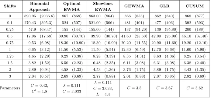
Table 2. The results of ARL1 study for ARL0= 865.
Shifts Binomial Approach
Optimal EWMA
Shewhart
EWMA GEWMA GLR CUSUM 0 890.95 (2036.6) 867 (868) 863.00 (864) 866 (853) 862 (840) 868 (877) 0.1 270.43 (395.3) 524 (507) 521.00 (506) 481 (401) 477 (406) 592 (593) 0.25 57.9 (68.47) 155 (144) 155.00 (144) 137 (94.20) 139 (95.80) 200 (188) 0.5 17.96 (17.58) 39.90 (30.70) 39.90 (30.70) 41.60 (25.60) 42.90 (25.90) 46.10 (37.40) 0.75 9.53 (6.98) 18.30 (10.90) 18.30 (10.90) 20.20 (11.55) 20.90 (11.60) 19.20 (12.10) 1 6.65 (3.12) 11.50 (5.53) 11.50 (5.54) 12.30 (6.59) 12.70 (6.68) 11.60 (5.90) 1.25 4.65 (2.29) 8.29 (3.38) 8.28 (3.39) 8.35 (4.31) 8.63 (4.36) 8.25 (3.54) 1.5 3.82 (1.52) 6.50 (2.23) 6.48 (2.35) 6.11 (3.08) 6.31 (3.08) 6.38 (2.40) 2 2.89 (0.94) 4.58 (1.32) 4.53 (1.36) 3.76 (1.75) 3.89 (1.75) 4.42 (1.35) 3 2.04 (0.57) 2.69 (0.69) 2.77 (0.88) 2.01 (0.88) 2.07 (0.85) 2.82 (0.69) Parameters C = 0:42,
C0= 1:8
= 0:111 C = 3:033
= 0:111 C = 3:033,
L = 4:4
that ARL0 is 470 in the simulation experiment. It
means that ARL0 is suciently large and, according
to ARL0 = 1, the probability of type-one error () is
suciently small. The value of c and c0has been chosen
to show the good performance of the proposed method. For the comparison study, we estimate the ARL1
and the standard deviation of the run lengths of the proposed method, as well as the optimal EWMA, She-whart EWMA, GEWMA, GLR and CUSUM methods, by 10000 independent replications in each scenario of the mean shifts. The shifts are given in multiples of the process standard deviations and are shown in the rst column of Table 1. The second up to the sixth column of Table 1 show the ARL1values of the methods under
consideration.
The results of Table 1 illustrate that the Binomial method performs better than other methods in all scenarios of mean shifts. In other words, not only the probability of type-one error, but also the probability of type-two error associated with the proposed method is less than their corresponding values in the other methods (according to formulas ARL1 = 1 1 and
ARL0 = 1 [17]). Moreover, the standard deviations
of ARL1 for the proposed methods are generally less
than these values in the other methods.
For the intended ARL0 865 in Table 2, we pick
c = 0:42 and c0 = 1:8, such that the ARL
0 for the
binomial method is 890 in the simulation experiment. In this case, we have the same conclusions as from Table 1. As seen from Tables 1 and 2, the GEWMA control chart is better than the other methods in detecting a large mean shift, but for mean shifts less than 3, the proposed method is the best.
AUTOCORRELATION
An autoregressive moving average model, denoted as ARMA(p; q), is often used to represent the autocorre-lation structure of the data. The general ARMA(p; q) model is:
xk = (B)(B)ak; (10)
where xk are observed data, ak are independent and
identically distributed (i.i.d.) normal variables with mean zero and variance, 2, and B is the backshift
operator. (B) and (B) are referred to as the AR and MA polynomial, and are parameterized as (B) = 1 '1B1 '2B2 'pBp and (B) =
1 1B1 2B2 qBq, respectively. Suppose there
is a deterministic shift which we refer to as a fault in the process at some time, . The process data to be monitored may be represented as:
yk = xk+ fk ;
where fk indicates the nature of the fault, and is the
fault magnitude. For a step mean shift (for example fk = 1 for k 0 and 0 otherwise), it is assumed that
the model in Equation 10 is invertible, the case in which the residuals can be obtained by ltering yk with the
inverse lter, (B)(B), that is: ek= (B)(B)yk = ak+ fk ;
where:
fk = (B)(B)fk ;
is referred to as the fault signature [18]. Thus, the residuals are uncorrelated with time-varying mean, fk , and variance, 2
e. The value of fk depends
on the ARMA model and, hence on the autocorrelation structure of the data.
The information in the dynamics of the fault signature can be useful for detecting faults. Traditional residual-based charts do not make use of this informa-tion, however. In contrast, a Generalized Likelihood Ratio Test (GLRT) or a cumulative score (Cuscore) chart can take this information into account [14].
The Cuscore test, originally introduced by Fisher [19], was later developed by Bagshaw and Johnson [20]. The Cuscore test is intended to detect changes in the parameters of a stochastic model. In some sense [14], the Cuscore chart is a form of the popular CUSUM control chart. The one-sided Cuscore statistic is:
Qk= maxfQk 1+ rk(ek m); 0g;
where rk and m are referred to as the detector and
reference values, respectively. If Qk exceeds a decision
interval, h, it is concluded that a fault has occurred in the process.
The model for rst-order autocorrelation (the AR(1) model) is the most frequently encountered case in practice. Therefore, we restrict our work to the AR(1) case. For this model, the choice of m = (1 1)2
is nearly optimal, in terms of minimizing the out-of-control ARL and rk= 1 1[21].
We know that the standard residuals, ek
e, follow a
standard normal distribution. Now, after determining the residuals, we consider three intervals for standard residuals, as follows:
I1= ( 1; 0:44); I2= ( 0:44; 0:44);
I3= (0:44; 1):
Statistics, xi;k i = 1; 2; 3 k = 1; 2; , are dened
ith interval among k gathered observations, and are calculated using the following recursive equation:
xi;k=
8 > < > :
xi;k 1+ 1 If the kth standard residuals ek
e is in interval Ii
xi;k 1 Otherwise (11)
Other mathematical derivations are similar to the pre-vious section and when one of the following inequalities is satised, the process is classied to be in an out-of-control condition.
1. For the initial observations, when k 15, if the statistics, Wk, are more than a constant threshold
like c, then the process is categorized to be out-of-control. Wk is the EWMA statistic of the standard
residuals and will be dened by the following equation:
Wk(r) = rek
e + (1 r)Wk 1(r);
15 > k > 0; W0(r) = 0;
2. In the case of gathering more than 15 observations, k > 15, when:
P3
i=1(xi;k xk)2
k > c0;
then the process is classied to be in an out-of-control condition.
The value of c and c0 should be determined to
ascertain a given probability of the type-one error. Results of the simulation study for dierent values of the autocorrelation coecient have been shown in Tables 3, 4 and 5.
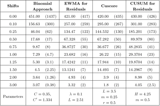
Table 3 shows the results of a comparison study for = 0:5. As seen, the proposed method performs better than the other methods in mean shifts that are in the interval (0; 2), and for shifts more than 2, the Cusum methods for residuals are the best, respectively. Also, the results in Table 3 denote that the standard deviation for ARL1 values in the proposed method is less than the ones in other methods.
Table 4 shows the results of the comparison for = 0:9. In this case, for shifts less than 0:1, the EWMA method is the best; the Cuscore chart being the best for detecting shifts between 0:1 and 1:5. For other mean shifts, the proposed method is the best. We know that when a shift, , occurs in the mean of an autocorrelated variable, then the value of shift in the residuals will be (1 ) [22]. Thus, the results of the simulation for case = 0:9 was expected, because shift 0:1 occurs in the mean of residuals, which is so much less than the real mean shift in the process. Also, the standard deviation of ARL values in the Cuscore method is the minimum for all mean shifts.
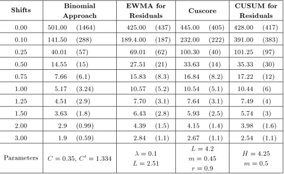
The results for = 0:1 have been shown in Table 5. In this case, for all shifts less than 2, the proposed method performs better than other methods and also its standard deviation is the least. For other mean shift, the Cuscore method has the best perfor-mance. Because of the low value of the autocorrelation, this result is expected.
Table 3. The results of ARL0 and ARL1 study for = 0:5.
Shifts Binomial Approach
EWMA for
Residuals Cuscore
CUSUM for Residuals 0.00 451.00 (1437) 421.00 (417) 420.00 (435) 430.00 (426) 0.10 156.63 (300) 257.00 (259) 295.00 (267) 301.00 (283) 0.25 46.04 (62) 134.47 (122) 144.532 (130) 185.201 (173) 0.50 17.68 (17) 67.328 (55) 67.282 (50) 89.979 (80) 0.75 9.87 (8) 36.8727 (30) 36.677 (26) 48.2835 (41) 1.00 7.29 (4.7) 23.682 (16) 26.22 (15) 29.3704 (23) 1.25 5.30 (3.1) 17.4242 (11) 17.944 (10) 19.8704 (14) 1.50 4.5 (2.25) 13.1241 (7) 14.493 (7) 14.2967 (9) 2.00 3.64 (1.26) 4.93 (4) 3.9 (4) 8.98 (5) 3.00 3.07 (0.38) 3.32 (2) 1.8 (2) 4.05 (2.5) Parameters C = 0:35,
C0= 1:334
= 0:1 L = 2:51
L = 3:5 m = 0:25
r = 0:5
H = 4:25 m = 0:5
Table 4. The results of ARL0 and ARL1 study for = 0:9.
Shifts Binomial Approach
EWMA for
Residuals Cuscore
CUSUM for Residuals 0.00 520.00 (1423) 418.00 (425) 443.00 (405) 426.00 (419) 0.10 488.63 (1324) 386.00 (397) 393.00 (35) 391.00 (383) 0.25 470.24 (1301) 330.35 (334) 285.02 (322) 358.11 (348) 0.50 315.13 (824) 268.02 (269) 201.48 (255) 301.27 (301) 0.75 184.09 (413) 211.28 (212) 146.79 (209) 256.89 (249) 1.00 123.84 (251) 177.96 (169) 115.40 (170) 217.42 (209) 1.25 90.14 (168) 144.45 (131) 88.62 (135) 183.75 (179) 1.50 72.18 (127) 116.64 (111) 72.97 (110) 160.25 (152) 2.00 47.1 (76) 85.93 (72) 82.9 (47) 118.98 (113) 3.00 26.2 (34) 51.32 (39) 55.8 (26) 63.05 (63) Parameters C = 0:35,
C0= 1:334
= 0:1 L = 2:51
L = 1:45 m = 0:05 r = 0:1
H = 4:25 m = 0:5
Table 5. The results of ARL0 and ARL1 study for = 0:1.
Shifts Binomial Approach
EWMA for
Residuals Cuscore
CUSUM for Residuals 0.00 501.00 (1464) 425.00 (437) 445.00 (405) 428.00 (417) 0.10 141.50 (288) 189.4.00 (187) 232.00 (222) 391.00 (383) 0.25 40.01 (57) 69.01 (62) 100.30 (40) 101.25 (97) 0.50 14.55 (15) 27.51 (21) 33.63 (14) 35.33 (30) 0.75 7.66 (6.1) 15.83 (8.3) 16.84 (8.2) 17.22 (12) 1.00 5.17 (3.24) 10.57 (5.2) 10.54 (5.1) 10.44 (6) 1.25 4.51 (2.9) 7.70 (3.1) 7.64 (3.1) 7.49 (4) 1.50 3.63 (1.8) 6.43 (2.8) 5.93 (2.5) 5.74 (3) 2.00 2.9 (0.99) 4.39 (1.5) 4.15 (1.4) 3.98 (1.6) 3.00 1.9 (0.59) 2.84 (1.1) 2.67 (1.1) 2.54 (1.1) Parameters C = 0:35, C0= 1:334 = 0:1
L = 2:51
L = 4:2 m = 0:45
r = 0:9
H = 4:25 m = 0:5
SENSITIVITY ANALYSIS ON THE NUMBER OF INTERVALS
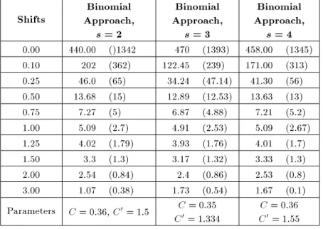
Although, in our study, the domain of the data was divided into three intervals, a question may be raised on the optimal number of partitioning intervals. To test the sensitivity of results to the number of intervals, a new simulation study is carried out. The simulation is tested using s = 2, 3, 4 intervals, and the ARL values are estimated using 10000 independent replications in each scenario of the mean shifts.
As can be seen from Table 6, changing the
number of the intervals has a low eect on the per-formance of the proposed approach in detecting an out-of-control process. Also, it can be seen that among simulated cases, partitioning the domain of the data into s = 3 intervals has a slightly better performance.
From a theoretical point of view, we know that in control process problems, three cases may occur: a negative shift, a positive shift, or no change in the process mean. Thus, dividing the domain of the data into three intervals is reasonable because each interval corresponds to a state of the process.
Table 6. The results of the sensitivity analysis on the number of intervals.
Shifts
Binomial Approach,
s = 2
Binomial Approach,
s = 3
Binomial Approach,
s = 4 0.00 440.00 ()1342 470 (1393) 458.00 (1345) 0.10 202 (362) 122.45 (239) 171.00 (313) 0.25 46.0 (65) 34.24 (47.14) 41.30 (56) 0.50 13.68 (15) 12.89 (12.53) 13.63 (13) 0.75 7.27 (5) 6.87 (4.88) 7.21 (5.2) 1.00 5.09 (2.7) 4.91 (2.53) 5.09 (2.67) 1.25 4.02 (1.79) 3.93 (1.76) 4.01 (1.7) 1.50 3.3 (1.3) 3.17 (1.32) 3.33 (1.3) 2.00 2.54 (0.84) 2.4 (0.86) 2.53 (0.8) 3.00 1.07 (0.38) 1.73 (0.54) 1.67 (0.1) Parameters C = 0:36, C0= 1:5 C = 0:35
C0= 1:334
C = 0:36 C0= 1:55
CONCLUSIONS
In this paper, we proposed a binomial distribution approach to analyze the cumulated data for a uni-variate quality characteristic. In this approach, we used a EWMA control method for initial observations. After gathering enough observations, we used an ap-proximation rule for evaluating binomial distribution with normal distribution and, then, dened a statistic, S2, that is the standard deviation of random normal
variables, xi;k i = 1; 2; 3. Since the probability
distribution function of S2is a 2distribution with two
degrees of freedom, we determined a constant control threshold for statistic S2, such that when the updated
statistic, S2, in dierent iterations of data gathering
process is more that a control threshold, the process is determined to be in out-of-control state.
Simulation experiments were carried out to com-pare the performance of the proposed method with ones of the optimal EWMA, GEWMA, CUSUM and GLR control charts. The results showed that the cumulative binomial method would improve the performance of process control techniques by decreasing the probabil-ity of type-one and type-two errors.
The primary assumption of this research was the independency of observations. For autocorrelated data, however, the proposed method was adapted for the residuals that were i.i.d variables. For this case, the results of the simulation study showed that the pro-posed method performs better than other methods for small to moderate values of autocorrelation coecients. We used an EWMA control method for initial observations. However, testing other methods is a good point for future research. Also, determining the optimal time of changing from the EWMA method
to the binomial approach is another good point for research. Moreover, a sensitivity analysis on the values of c and c0 is required.
ACKNOWLEDGMENTS
The authors would like to thank the referees for their valuable comments and suggestions, which improved the presentation of this paper.
REFERENCES
1. Niaki, S.T.A. and Fallahnezhad, M.S. \Decision-making in detecting and diagnosing faults in multivari-ate statistical quality control environments", Interna-tional Journal of Advanced Manufacturing Technology, 42(7), pp. 713-724 (2009).
2. Hunter, S.J. \The exponentially weighted moving av-erage", Journal of Quality Technology, 18, pp. 203-210 (1986).
3. Crowder, S.V. \A simple method for studying run-length distributions of exponentially weighted mov-ing average charts", Technometrics, 29, pp. 401-407 (1987).
4. Wu, Y.H. \Design of control charts for detecting the change point", in Change-Point Problems, E. Carl-stein, H.G. Muller and D. Siegmund, Eds., pp. 330-345, IMS, Hayward, CA (1994).
5. Han, D. and Tsung, F. \A generalized EWMA control chart and its comparison with the optimal EWMA, CUSUM and GLR schemes", The Annals of Statistics, 32(1), pp. 316-339 (2004).
6. Page, E.S. \Continuous inspection schemes", Biometrika, 14, pp. 100-115 (1954).
7. Woodall, W.H. \The design of CUSUM quality control charts", Journal of Quality Technology, 18, pp. 99-101 (1986).
8. Siegmund, D. and Venkatraman, E.S. \Using the generalized likelihood ratio statistic for sequential de-tection of a change-point", The Annals of Statistics, 23, pp. 255-271 (1995).
9. Marcellus, R.L. \Bayesian monitoring to detect a shift in process mean", Quality and Reliability Engineering International, 23, pp. 233-245 (2007).
10. Fallahnezhad, M.S. and Niaki, S.T.A. \A new moni-toring design for uni-variate statistical quality control charts", Information Sciences, 180, pp. 1051-1059 (2010).
11. Box, G.E., Hunter, W.G. and Hunter, J.S. \Statistics for experimenters: An introduction to design, data analysis, and model building", Wiley-Interscience, 2nd Ed., p. 53 (2005).
12. Lu, C.W. and Reynolds, M.R. \EWMA control charts for monitoring the mean of autocorrelated processes", Journal of Quality Technology, 31, pp. 166-188 (1999). 13. Lu, C.W. and Reynolds, M.R. \CUSUM charts for monitoring an autocorrelated process", Journal of Quality Technology, 33, pp. 316-334 (2001).
14. Shu, L., Apley, D.W. and Tsung, F. \Autocorrelated process monitoring using triggered CUSCORE charts", Quality and Reliability Engineering International, 18, pp. 411-421 (2002).
15. Srivastava, M.S. and Wu, Y.H. \Comparison of EWMA, CUSUM and Shiryayev-Roberts procedures for detecting a shift in the mean", The Annals of Statistics, 21, pp. 645-670 (1993).
16. Srivastava, M.S. and Wu, Y.H. \Evaluation of op-timum weights and average run lengths in EWMA control schemes", Comm. Statist. Theory Methods, 26, pp. 1253-1267 (1997).
17. Montgomery, D., Introduction to Statistical Quality Control, John Wiley and Sons, Inc., 4th Ed. (2001). 18. Apley, D.W. and Shi, J.J. \The GLRT for
statisti-cal process control of autocorrelated processes", IIE Transactions, 31, pp. 1123-1134 (1999).
19. Fisher, R.A. \Theory of statistical estimation", Pro-ceedings of the Cambridge Philosophical Society, 22, pp. 700-725 (1925).
20. Bagshaw, M. and Johnson, R.A. \Sequential pro-cedures for detecting parameter changes in a time-series model", Journal of the American Statistical Association, 72, pp. 593-597 (1977).
21. Hu, S.J. and Roan, C. \Change patterns in the time series-based control charts", Journal of Quality Technology, 28, pp. 302-312 (1996).
22. Wieringa, J.E. \Statistically process control for seri-ally correlated data", PhD Thesis, Rijksuniversiteit Groningen (1999).
BIOGRAPHIES
Mohammad Saber Fallah Nezhad graduated from Sharif University of Technology, Iran. His research area is focused on Quality Control. He is also interested in Stochastic Modeling, Dynamic Programming and Sequential Analysis. Dr. Fallah-Nezhad is Assistant Professor of Industrial Engineering at Yazd University, Iran.
Mohammad Saleh Owlia is Associate Professor of Industrial Engineering at Yazd University, Iran. He obtained his B.S. and M.S. degrees from Sharif University of Technology, Tehran, Iran and his Ph.D. in Quality Management from Birmingham University, in the UK. Dr. Owlia's research has focused on Quality Management and Engineering, Performance Assess-ment, and Knowledge Management. He is recipient of both a distinguished researcher award, and outstanding lecturer award from Yazd University.