GO-SHIP Repeat Hydrography Nutrient Manual:
The precise and accurate determination of dissolved inorganic nutrients in seawater, using
Continuous Flow Analysis methods.
Susan Becker1, Michio Aoyama2, E. Malcolm S. Woodward3, Karel Bakker4, Stephen Coverly5, Claire
Mahaffey6, Toste Tanhua7.
1. UC San Diego, Scripps Institution of Oceanography, 9500 Gilman Dr. MC 0236, San Diego, CA 92093, USA. 2. RIGC, JAMSTEC, 2-15 Natsushima, Yokosuka, 237-0061, and CRIED, University of Tsukuba, 305-8572, Japan. 3. Plymouth Marine Laboratory, Prospect Place, The Hoe, Plymouth, PL1 3DH. United Kingdom.
4. NIOZ, Royal Netherlands Institute for Sea Research, Department of Ocean Science, and Utrecht University, PO Box 59 Den Burg 1790 AB, The Netherlands.
5. BLTEC, #1607, 1 Dong, 775, Gyeongin-Ro Yeongdeungpo-Gu, Seoul, 150-972, Korea.
6. Department of Earth, Ocean and Ecological Sciences, SOES, University of Liverpool, Liverpool, L69 3GP. United Kingdom.
7. GEOMAR Helmholtz Centre for Ocean Research Kiel, Duesternbrooker Weg 20, D-24105 Kiel, Germany.
Acknowledgements:
This Nutrient Manual was written and revised by members of WG 147: Towards comparability of global oceanic nutrient data (COMPONUT) of the Scientific Committee on Oceanic Research (SCOR).
Support for this work was provided by the U.S. National Science Foundation (Grants 1546580 and OCE-1840868), national SCOR committees, and other sources.
The authors thank the contributions made by other WG #147 members:
Andrew Dickson, Bernadette Sloyan, Karin Bjorkman, Anne Daniel, Hema Naik, and Raymond Roman. Thank you also to numerous other scientific colleagues who reviewed the manuscript and provided helpful comments and suggestions for improvements.
Table of Contents:
1. Introduction ... 4
1.1 Nutrient Data Comparability: GEOSECS to GO-SHIP ... 4
1.2 Methods and Instrumentation... 5
2. Sample Collection and Storage ... 6
2.1 Sample collection ... 6
2.2 Filtering and gloves ... 6
2.3 Sample Preservation... 7
3. Instrumentation ... 7
3.1 Sampler ... 7
3.2 Pump ... 8
3.3 Manifold ... 8
3.4 Detectors ... 9
3.5 Software ... 9
4. Measurement and determination of nutrient concentrations: ... 9
4.1 Baseline determinations ... 9
4.2 Calibration ... 10
4.3 Measurement of sample peak heights ... 10
4.4 Corrections for any baseline drift, sensitivity drift, and carryover ... 11
4.5 Determination of initial concentrations of samples ... 11
4.6 Post processing corrections ... 11
5. Chemical analytical Methods ... 11
5.1 Nitrate and Nitrite Analysis ... 11
5.2 Phosphate Analysis ... 12
5.3 Silicate Analysis ... 12
5.4 Ammonium Analysis: ... 12
6. Standard Preparation and Standardization ... 12
6.1 Primary Standards ... 13
6.2 Secondary (Sub-primary) Standards ... 14
6.3 Working standards ... 14
7. Quality Control and Quality Assessment (QC/QA): ... 14
7.1 Definitions and Determination ... 14
7.2 Standard Operating Procedures (SOPs) ... 15
7.3 Internal Checks: ... 16
7.4 External Quality Checks: ... 16
7.5 Data Quality Assessment ... 18
8. Documentation ... 18
8.1 Cruise reports ... 18
8.2 Bottle data files: ... 18
References: ... 20
Appendix A: ... 23
Applying air buoyancy corrections ... 23
Appendix B: ... 27
Appendix C: ... 30
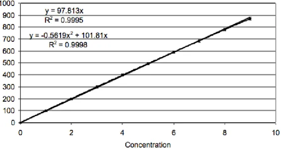
Establishing the linearity of standard calibrations ... 30
Appendix D: ... 35
Low-level (nanomolar) nutrients ... 35
Appendix E: ... 37
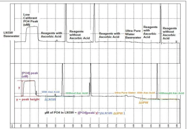
Determination of nutrient concentrations in LNSW or ASW ... 37
Appendix F: ... 39
Detailed methods utilized at SIO for AA3 ... 39
Appendix G: ... 47
Detailed methods for QuAAtro 2-HR utilized at JAMSTEC ... 47
Appendix H: ... 53
Experimental results: NIOZ and SIO sample freezing and thawing on silicate results... 53
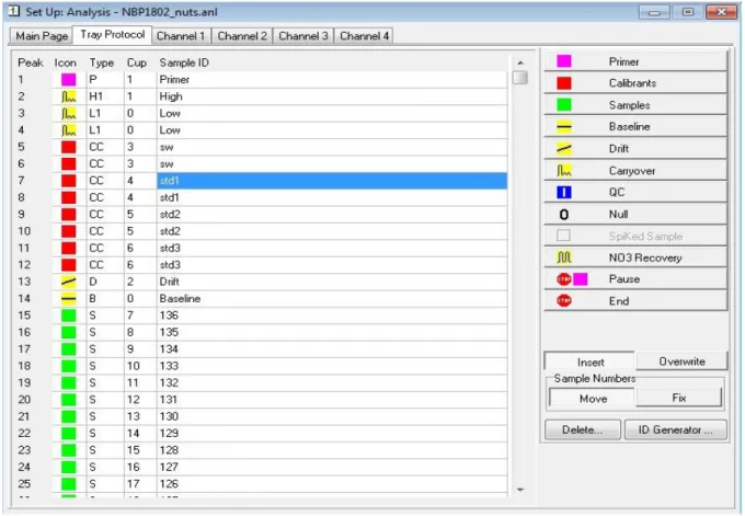
List of Figures and Tables: Figure 1. An example of a tray file. ... 15
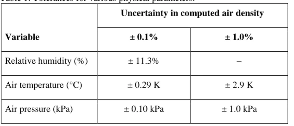
Table 1: Tolerances for various physical parameters... 23
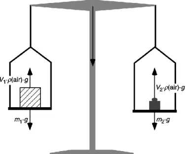
Figure 2. Forces on sample (1) and weights (2) when weighing in air. ... 25
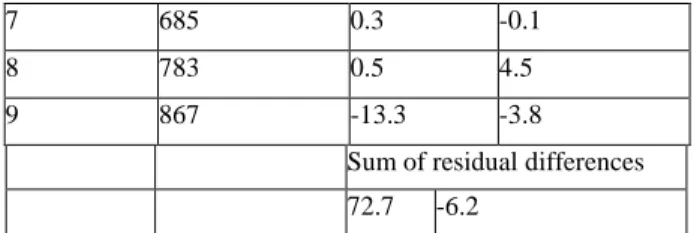
Table 2: Data for linearity check. ... 32
Figure 3: Plot of analyzer data from Table 2. ... 33
Figure 4: Plot of the residual difference ... 33
Figure 5: Determination of Phosphate concentration in LNSW ... 37
Figure 6: SIO Nitrate flow diagram ... 42
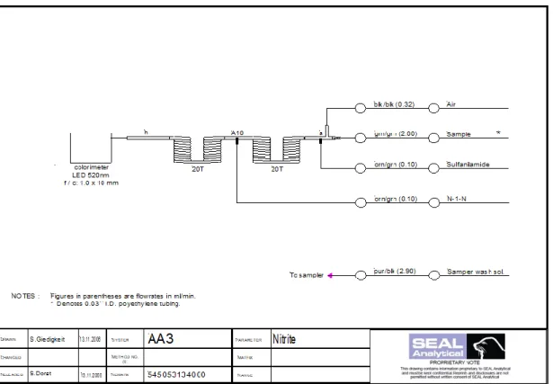
Figure 7: SIO Nitrite flow diagram... 42
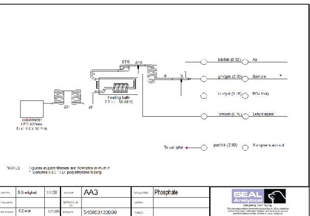
Figure 8: SIO Phosphate flow diagram ... 43
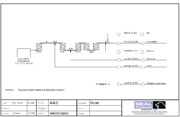
Figure 9: SIO Silicate flow diagram ... 44
Figure 10: SIO Ammonium flow diagram ... 46
Figure 11: JAMSTEC Nitrate plus Nitrite flow diagram. ... 47
Figure 12: JAMSTEC Nitrite flow diagram ... 48
Figure 13: JAMSTEC Silicate flow diagram. ... 49
Figure 14: JAMSTEC Phosphate flow diagram. ... 50
Figure 15: JAMSTEC Ammonium flow diagram. ... 52
Figure 16: Results of different thaw techniques on silicate concentrations ... 54
Figure 17: Silicate results from thawing at 50C. ... 54
Figure 18: Nitrate plus Nitrite results from thawing at 50C. ... 55
GO-SHIP Repeat Hydrography Nutrient Manual:
The precise and accurate determination of dissolved inorganic nutrients in seawater using Continuous Flow Analysis (CFA) methods.
1. Introduction
This GO-SHIP manual is an update to the original version by Hydes et al. (2010), and reviews basic sample collection and storage, aspects of CFA using an Auto-Analyzer, and specific nutrient methods in use by many laboratories doing repeat hydrography. The document also covers laboratory best practices including quality control and quality assurance (QC/QA) procedures to obtain the best results, and suggests protocols for the use of reference materials (RM) and certified reference materials (CRMs).
1.1 Nutrient Data Comparability: GEOSECS to GO-SHIP
The availability of inorganic macronutrients (nitrate (NO3), phosphate (PO4), silicic acid (Si(OH)4) commonly
referred to as ‘silicate’, ammonium (NH4), and nitrite (NO2)) in upper ocean waters frequently limits and regulates
the amount of organic carbon fixed by phytoplankton, thereby constituting a key control mechanism of carbon and biogeochemical cycling. There are a number of biogeographic regions in the open ocean characterized by different macronutrient regimes, either permanently or seasonally limiting the growth of phytoplankton (Moore 2016). Accurately measuring temporal changes in macronutrient concentrations is essential to constraining net biological production and export fluxes, detecting shifts in biogeographic regimes, and for monitoring eutrophication
phenomena. For open ocean work an analytical accuracy of 1% should be aimed for by the Global Ocean Ship-based Hydrographic Investigations Program (GO-SHIP) (Talley et al., 2016) to allow reliable quantification of decadal trends in the deep ocean. An internal consistency of nutrient data in the order of 1 - 3% has been achieved through secondary quality control (QC) procedures implemented in the Global Ocean Data Analysis Project (GLODAPv2: Olsen et al., 2016).
The Geochemical Ocean Sections Study (GEOSECS) in the 1970s was one of the first efforts to provide a global survey of chemical, isotopic, and radiochemical tracers in the world’s oceans. Since then there have been numerous international collaborations to map and study different chemical, physical, and biological aspects of the oceans. These programs include the Joint Global Ocean Flux Study (JGOFS) in the late 80s, World Ocean Circulation Experiment (WOCE) in the mid to late 90s, and the current global programs including, Climate Variability and predictability (CLIVAR), GEOTRACES, and GO-SHIP. In addition to these large international efforts, there continues to be many other programs led by individual laboratories and countries to study specific areas and processes in the world’s oceans, including ocean time-series stations and transects.
All of these efforts have led to large data synthesis studies, including Carbon dioxide in the Atlantic Ocean (CARINA, Key et al. 2010) Pacific Ocean Interior Carbon (PACIFICA, Suzuki et al. 2013), GLODAPv1, and GLODAPv2. These studies include analysis from different international laboratories. It is imperative that the data sets produced by the different laboratories are comparable, and differences in concentrations in time or space are real and not artifacts of differing methods, standards or instrumentation. In an effort to verify the comparability of nutrient data sets there have been a number of inter-laboratory comparability exercises(UNESCO 1965, 1967; ICES 1967, 1977; Kirkwood et al. 1991; Aminot and Kirkwood 1995). There are commercially available nutrient stock standard solutions, e.g. OSIL (http://osil.com/), and other programs supply stock standard solutions that allow laboratories to validate their methods (Topping 1997). However, there was a need for a reference material for nutrients that would allow laboratories to compare and closely monitor data quality.
There have been inter-laboratory comparison studies using reference materials with one of the first being MOOS certified by the National Oceanic and Atmospheric Administration/ National Research Council Canada
(NOAA/NRC). The Meteorological Research Institute (MRI) in Japan has led a more recent series of international inter-laboratory comparisons in 2003, 2006, 2008 and 2012 (Aoyama 2006, 2007, 2008, and 2010). The motivation of the exercises led by MRI was the development of reference materials for nutrients in seawater (RMNS). In 2014/2015 and 2017/2018 the International Ocean Carbon Coordination Project (IOCCP) and Japan Agency for Marine-Earth Science and Technology (JAMSTEC) conducted inter-laboratory comparison studies of nutrient CRMs in seawater. These two intercomparison exercises used CRMs as known samples in 2014/2015 (Aoyama et
al. 2016), or as unknown samples in 2017/2018. The availability and use of these CRMs has been instrumental in improving the global comparability of nutrient data sets. These recent exercises were carried out as part of the terms of reference of the International SCOR working group #147: Towards comparability of global oceanic nutrient data (COMPONUT); (http://www.scor-int.org/SCOR_WGs_WG147.htm).
1.2 Methods and Instrumentation
The basic analytical methods and chemistries that are used to determine concentrations of inorganic nutrients in seawater are well established. Strickland and Parsons outlined the manual methods in their book, “A Practical Handbook of Seawater Analysis” (Strickland and Parsons, 1972). The chemical methods have been changed, optimized and automated over the decades by numerous authors, but the basic chemistries remain the same and are based on colorimetric reactions. The exception to this is the newer methods for ammonium/ammonia determination, which are based on fluorometry.
Nitrate is determined using a procedure described byArmstrong et al. (1967), which involves passing a seawater sample through a copper-cadmium reduction column where the nitrate is reduced to nitrite. Nitrite is then diazotized with sulfanilamide and coupled with N-1-naphthyl-ethylenediamine dihydrochloride (N-1-N/NEDD) to form a red azo dye, and the absorbance is measured between 520 and 540nm.
Phosphate is determined by adding acidified ammonium molybdate to the seawater sample to produce
phosphomolybdic acid, which is then reduced to a phospho-molybdenum blue complex following the addition of dihydrazine sulfate (Bernhardt and Wilhelms 1967), or ascorbic acid (Murphy and Riley 1962), which was optimized by Zhang et al. (1999). The absorbance is measured between 850 and 880nm.
Silicate is analyzed according to two methods. The method outline in Armstrong (1967) produces a silicomolybdic acid with the addition of ammonium molybdate. A silico-molybdenum complex is then formed following the addition of stannous chloride, and the absorbance is measured at approximately 660nm. Alternatively the method published in Grasshoff et al. (1983) uses ascorbic acid to reduce the silicomolybdic acid to the blue complex, and the absorbance is measured at approximately 820nm.
There are two commonly used ammonium methods, colorimetric and Fluorometric. The colorimetric method uses the Berthelot reaction, and involves the reaction of hypochlorite and phenol with ammonium in an alkaline solution to form an indophenol blue compound. The sample absorbance is measured at approximately 660nm. This method is a modification of the procedure in Grasshoff (1983). The highly sensitive Fluorometric method using ammonia diffusion across a teflon membrane with Fluorometric detection (Jones, 1991) was developed, but obtaining the membrane proved difficult. A simplified technique using fluorometry but without the use of a membrane, was published by Holmes et al. (1999), which was adapted from Kerouel and Aminot (1997). In this method, the seawater sample is combined with a working reagent containing ortho-phthaldialdehyde (OPA), sodium sulfite, and borate buffer, and heated to 75°C. Fluorescence proportional to the ammonium concentration, emission at 460nm following excitation at 370nm is measured.
Laboratories started using CFAs and Auto-Analyzers (AA) in the mid-1970s. The two main forms of CFA are flow injection (FIA) and gas-segmented flow analyzers. While there are some laboratories that are using FIA for nutrient analysis, most global laboratories that carry out ‘at-sea’ analysis use gas-segmented flow analyzers. This manual focuses primarily on methods for the gas-segmented flow analyzers.
The chapter on nutrient analysis using segmented flow analysis by Aminot et al. (2009) in “Practical Guidelines for the Analysis of Seawater”provides an excellent background on continuous flow analysis. We recommend the reader also review this document as it contains useful information on the technical aspects of the instrument(s), the
2. Sample Collection and Storage
2.1 Sample collection
The Data Acquisition Overview section of the GO-SHIP (Swift 2010) manual should be reviewed for details on rosette/Niskin bottle sampling practices. Nutrient samples should be collected from the Conductivity Temperature Depth (CTD) rosette/Niskin bottles immediately after the collection of samples for dissolved gases. This can be challenging if samples for organic properties or biologically sensitive materials are also being taken. Ideally, samples are collected into new, sterile plastic (High Density Polyethylene (HDPE), or Polypropylene (PP) containers that will then fit directly onto the AA auto-sampler, or sub-sampled into smaller containers. Sample containers can be re-used if proper cleaning procedures are followed between stations. Using a new sample container could produce a tremendous amount of plastic waste especially on the long repeat hydrography research cruises and these environmental impacts should be considered. For macro-nutrient analysis (micro-molar (µM) concentrations), rinsing the sample containers with ultrapure water (distilled deionized water or from commercially available systems) followed by a rinse with 10% Hydrochloric Acid (HCl, 1.2M) is sufficient. This stops any biological growth in the sample bottles. These then should be rinsed well with ultrapure water prior to the collection of the next set of samples. Glass sample containers should not be used if measuring silicate. If nanomolar nutrient concentrations are being measured, other cleaning and sample collection procedures will be necessary (see Appendix D).
When taking the seawater samples from the CTD/rosette bottles, rinse the clean sample containers and caps three times before filling. Avoid touching the sampling spigots on the CTD bottles and take care to rinse the spigots as well as the nutrient sample containers. Samples can be collected with the use of a Tygon or silicon sampling tube. If a sampling tube is used, rinse it thoroughly before going out to the rosette to take a series of samples, and make sure to rinse it with each seawater sample prior to collecting the sample. Once rinsed, fill the sample containers two thirds full, and cap immediately. The samples should be analyzed after they have equilibrated to the laboratory room temperature. If analysis will be delayed for longer than a couple of hours (>2), then store the samples in a dark and cool place, for example in a refrigerator, however the samples should be returned to room temperature before analysis. Between CTD sampling events it is important to clean any sampling tubes with clean deionized water and 10% HCl.
N.B. Cigarette smoke can contaminate samples, particularly for ammonium and nitrate/nitrite, so it is imperative that smoking is banned close to the area where samples are collected. Likewise, people who have been recently smoking should stay away from any open samples.
2.2 Filtering and gloves
Some laboratories filter nutrient samples, while many other laboratories do not. In general, filtering is not necessary for samples taken in the (sub) tropical open ocean, where particle loading is low in these oligotrophic environments. The decision to filter or not is dependent on the particulate loading in the water being sampled. For example, samples from near shore or productive environments may require filtering. In these cases, great care must be taken not to contaminate the samples during the sample handling and filtering process. Sample collection tubes, filter holders, and filters should be clean and well rinsed with 10% HCl and ultrapure water prior to sample collection. Types of filters used to filter seawater include cellulose acetate, hydrophilic polypropylene Gelman membrane, and Acrodisc syringe filters (PALL). Glass Fiber filters (GFF) (silicate contamination) or cellulose nitrate filters (nitrate contamination) should NOT be used. Filter size is another consideration, a filter with a pore size of 0.45µm is commonly used, and in the past this was considered the ideal filter size to remove the majority of particles. However, new insight from microscopy and genomics has determined that a 0.45µm filter does not capture all bacteria and phytoplankton. A 0.2µm filter is now the recommended size of filter, and gravity, low pressure, or low vacuum filtration is recommended to avoid cell rupture and sample contamination. It is imperative that tests are performed to check that the method of filtering, filter type, and filter size do not lead to contamination of the samples. Another simple technique to minimize particle interferences is to centrifuge the samples prior to analysis.
Gloves are another source of potential contamination. Neither Neoprene nor colored nitrile gloves should ever be used for the sampling of nutrients; they are a high source of contamination especially for nitrate, nitrite and
ammonium. If care is taken, a clean sample can be collected with bare hands without the use of gloves, however, powder free vinyl gloves are highly recommended for use in the lab and for sample collection at sea.
In general, it is best practice to wear gloves when taking water samples and only experienced scientists who are confident in their techniques should consider sampling without gloves. Likewise, it is important that for any sampling procedures (like gas sampling) being carried out prior to the nutrient sampling from the CTD, then those scientists should also wear non-nutrient contaminating gloves (e.g. powder free vinyl).
2.3 Sample Preservation
The best practice is to analyze the nutrient samples at sea, shortly after they are collected, however there are often instances when nutrient analysis at sea is not possible or is delayed for any number of reasons. If analysis will be delayed by more than 24 hours the samples must be preserved. There are many different types of preservation methods, including poisoning, acidification, pasteurization (Daniel et al. 2012), and freezing. We do not recommend acidification (samples will have to be neutralized before analysis) or poisoning samples with mercuric chloride (environmental hazard). Freezing is the most commonly used method, and there are studies that show that freezing can be a reliable method of sample preservation (Aminot and Kerouel1995; Dore et al. 1996), and this is the recommended procedure.
If freezing samples, it is imperative that there is sufficient headspace in the bottles to allow for expansion of the seawater. Freeze the samples upright and check that the caps are tightened before and after the samples have frozen. Do not freeze samples in a freezer that has had organic material (fish samples or food) stored in it. Analyze frozen samples as soon as possible after returning to the lab.
There is still debate within the nutrient community about the effects of freezing samples on the accuracy and precision of the nutrient concentration, especially for silicate. It is well known that the reactive silica polymerizes when frozen, especially at high concentrations (Burton et al. 1970; MacDonald and McLaughlin 1982; MacDonald et al. 1986). Variables that affect the recovery of silica from frozen samples include salinity, turbidity, bottle size, and the silicate concentration. Much of the current debate centers on the recommended thaw techniques to depolymerize the reactive silica and get complete recovery. Many laboratories have carried out studies of thaw techniques to recover silica, but there are only a few published references. Sakamoto et al. (1990) recommend that samples be thawed overnight, in the dark, at room temperature, or thawed in a water bath for 30 minutes (50˚C) and then cooled back down to room temperature before actual analysis. However, Zhang and Ortner (1998) suggested that it could take up to 4 days to thaw samples at room temperature to get complete recovery of silica. See appendix H for results of recent studies performed at NIOZ and Scripps Institution of Oceanography (SIO). The tests carried out at SIO confirm the 1990 recommendation by Sakamoto of thawing frozen samples in a 50˚C water bath for 30-45 minutes and then allowing the samples to come back to room temperature before analysis. Further systematic tests are needed to determine the effects of long term storage on all of the nutrient concentrations as well as the best thaw techniques for the different types of samples being collected (coastal, estuarine, oligotrophic, etc.)
3. Instrumentation
Aminot et al. (2009)provide a detailed description of the specific AA components, including potential problems of analysis. Most seagoing laboratories are using SEAL, Skalar, Alpkem, or similar analytical systems. Users should refer to the manufacturer's manuals for the specifics on methods, operation, and maintenance. A nutrient auto-analyzer from any manufacturer will consist of the same basic components listed and described here. 3.1 Sampler
The sampler should be robust and able to handle different size sample cups and a reasonable number of samples, plus it should have a wash from which the water is continuously refreshed. A non-metallic or platinum probe should be used, and the internal diameter of the probe should normally be no greater than that of the largest sample pump tube. Having a sampler modified to accept the bottles that you sample straight from the CTD rosette will eliminate possible contamination issues when decanting a sample into another sampling vessel.
3.2 Pump
The peristaltic pump delivers the sample/baseline water, and the reagents to the manifolds for each
channel/chemistry and throughout the entire AA system. For precise measurements at low concentrations, a regular bubble pattern and stable baseline are absolutely key, and this is one area that is extremely important to get correct for good analyses.
The composition and quality of pump tubes can vary between manufactures and from batch to batch. Tube wear will also affect the flow rate and method sensitivity, which is why a complete set of standards must be run with every station/set of samples. Replacing a method’s pump tubes may then improve the sensitivity and characteristics of the bubble flow. Generally, pump tubes should be changed on a regular basis as the correct delivery of the sample, and particularly for some reagents being pumped through some of the smaller bore pump tubes (e.g. orange/green or orange/yellow), will become a lot less accurate as the tubes wear. For optimum performance, changing tubes after 50-60 hours (depending on the material and manufacturer of the pump tubes in use) will ensure that the liquid delivery remains reliable. The newer phthalate-free pump tubes being sold have a much-reduced reliable life span compared to the original Tygon tubing. It is not good practice to run pump tubes right to the end of their useable life. The analytical results will not be as good or reliable with old tubes as with newer tubes, thus frequent changing of pump tubing is recommended. Some laboratories make a full change of pump tubes and reagents at the same time to co-ordinate machine down time.
3.3 Manifold
The manifold consists of glassware and injection fittings and is the site of the chemical reactions between the seawater samples and reagents. It is imperative that the glass pieces, reaction coils, and connectors are all maintained regularly in order to provide consistent mixing, regular flow patterns and to allow reactions to reach steady state, which ensures full color development.
Introduction of air or nitrogen bubbles allows for complete mixing between segments and again ensures full color development. The bubbles must be large enough to prevent carryover and/or smearing from one segment to another, but if they are too long they will be prone to breaking up in the manifold. It is very important to maintain a regular bubble pattern throughout the system in order to reduce noise and optimize sensitivity. Reference is always made to the segmented gas bubbles as being ‘air’ bubbles, however ideally these segmenting bubbles should be either nitrogen or another inert gas so as to avoid potential contamination from the air. Some laboratories have gas lines connected directly from cylinders to deliver the gas, but a simpler solution is to use small plastic Tedlar bags (or similar) that contain up to 5 liters of nitrogen. These are particularly useful when working at sea as they can be easily refilled.
There are many factors to consider when building a manifold to ensure consistent flow and bubble pattern. Below is a list of considerations:
1. Match the inner diameter (ID) of the tubing used from the pump to the injection fittings and into the glassware on the manifold as closely as possible.
2. Use the shortest possible length of tubing between connections. Long un-segmented streams cause hydraulic problems, which will manifest in various ways (e.g. smearing or carryover of samples). 3. Make sure there are no gaps/dead spaces between connections. It is important that all glass to glass joints
are held close together by plastic sleeving.
4. Add enough wetting agent in each analytical channel to maintain rounded edges at the front and back of each bubble throughout the entire flow stream, including the drain to waste.
5. Segmentation bubbles must completely fill the tubing through which they pass. The length of bubble in contact with the tubing walls should be approximately 1.5 times the tubing diameter.
6. Maintain the cleanliness of the glass coils to ensure smooth flow of the sample and reagent stream. Dirty glass can cause bubbles to stick or break up.
7. Clean the manifolds periodically with a phosphate-free laboratory detergent and consult the manufactures recommendations. A dilute bleach or acidic solution can also be used for nitrate, nitrite and ammonium. Silicate and phosphate channels can be cleaned with a dilute sodium hydroxide plus
ethylenediaminetetraacetic acid (EDTA) solution. Many analytical problems will be avoided with a regular cleaning protocol.
8. The segmented flowcell waste line should open to the atmosphere at about bench or flowcell height. 9. Replace any old glass pieces that continue to cause the air bubbles to stick or break up. Glass tubing and
3.4 Detectors
The detectors consist of a light source (e.g. lamp, light emitting diode (LED)), flowcell, photometer, and inlet and outlet tubing (either plastic or glass). As with the manifold, there should be no gaps at the connections, and there should be a regular bubble pattern maintained from the manifold through the detector unit to waste. Depending on the manufacturer, the ability to monitor changes in light output, voltage, and other variables through the software may be available, and should be utilized. In the past the sample flow was always de-bubbled immediately prior to the sample entering the flowcells, but now software developments from some manufactures have allowed the air bubbles to also pass through the cells eliminating the need to de-bubble. The ability to retain the bubble pattern through the flowcell reduces carryover and sample-to-sample smearing. This along with the optical design of the new photometers and flowcells have nearly eliminated the need for refractive index blanks (RIBs), and some other effects that have interfered with peak detection in the past. For more details on these corrections see section 4.6. 3.5 Software
The AA will come installed with software from the manufacturer to control the entire system, program the autosampler, acquire the raw data output from the detectors, display the output real-time, and perform some corrections, and calculate initial concentration values etc.
There are usually different options for the calibration fit to use within the software packages. If using a linear fit or higher order fit, the concentration of nutrients in the matrix and blanks for both the matrix and the samples, must be carefully determined and corrected for. Most software programs will correct for carryover, baseline, and sensitivity drifts but may not have options to make other corrections such as RIBs or non-zero matrix concentrations. Please refer to the software manual for your own type of analyzer to learn the specifics for your instrument.
Calibration fits and blank corrections are discussed in more detail later (Appendix C).
4. Measurement and determination of nutrient concentrations:
The basic steps for sample analysis include:
1) a. Establish a steady baseline with ultrapure water.
b. Establish a steady baseline with ultrapure water plus reagents.
c. Check the reagent blank (difference between ultrapure water and ultrapure water plus reagents). 2) Calibration curve determination from standard concentrations and measured peak heights. 3) Measurement of sample peak heights.
4) Corrections for carryover, baseline and sensitivity drift.
5) Determination of initial concentrations of samples based on calibration curve and sample peak heights. 6) Application of other corrections including RIBs, salt effect, etc.
4.1 Baseline determinations
A common baseline solution used throughout the nutrient analysis community is ultrapure fresh water. However, in some cases analysts use low nutrient seawater (LNSW) if they have plentiful supplies. Some labs make their own ‘artificial’ seawater, (ASW) by adding salts to ultrapure water. An example of a recipe for ASWis41g of sodium chloride plus 168mg of sodium bicarbonate per liter. Here we discuss using ultrapure water as the baseline water as this is a reliable and recommended ‘zero’ for nutrients, and can be obtained easily and quickly within a research laboratory. Determination of the baseline should be straightforward if the correct procedures are followed. The ultrapure water should be at least 18.2 megohm resistance, and be free of organics. Ultraviolet (UV) sterilization is preferred but not strictly necessary. Most commercially available water purification systems will provide ultrapure water that is acceptable for establishing a zero baseline. It should be noted that the wash pot on the sampler and the container that feeds into the wash pot can become contaminated. It is recommended that they be cleaned once per day by rinsing with 10% HCl solution followed by rinsing with ultrapure water. Some manufacturers offer a ‘travelling washpot’, which is a sealed system and hence stays uncontaminated and clean during daily operations so could be an option to consider. In rare cases it is possible that the ultrapure water is not pure, even if the resistivity reading is 18.2 megohm, e.g. silicate can pass through the filtration cartridge but will not affect the megohm reading.
It can be difficult to determine if the ultrapure water is not as pure as required and so analysts should be comparing the difference between the ultrapure baseline and the ultrapure baseline with reagents on a daily basis. Another possible indicator of poor quality baseline water is negative absorbance readings for samples with low nutrient concentrations. This could indicate the filtration cartridges on the ultrapure water system need to be replaced. The water baseline is determined after the instrument has been running long enough with fresh ultrapure water and the baselines have become stable. This also enables checking for any leaks throughout the system before the reagents are added. It may be necessary in rare cases to add wetting agent to the ultrapure water to establish a good bubble pattern and stable baselines. Once the ultrapure water baseline has stabilized, the reagents can be added and the reagents plus ultrapure water baseline determined. It is often useful to add the reagents one at a time to see if any of them cause a large reagent blank. The reagent baseline is the reference for when the standard curve is determined and the subsequent calculation of sample concentrations. It is good practice to define a regular setting up procedure for the analyzer that can be followed for every day and every run. To minimize the reagent blank, analytical grade (or better) chemicals and fresh ultrapure water should be used.
It is crucial that the nutrient concentrations for LNSW or ASW are calculated if they are being used as a baseline instead of ultrapure water. Aoyama et al. (2015) detailed a procedure which includes analyzing a known value of each standard added to the LNSW, followed by a baseline of LNSW with and without color reagent, and a baseline of ultrapure water with and without reagent. The differences are used to calculate the concentration of each nutrient in LNSW. See Appendix E for details.
There are different ways to obtain LNSW. One option is to collect large batches of surface seawater from oligotrophic waters during a research cruise. It is recommended that the water then be filtered and sterilized to ensure the nutrient levels remain low, e.g. pumped through a 0.45µm filter, past a UV light source, and then through a 0.1µm filter, and re-circulated for approximately16 hours. Alternatively, it is possible to collect surface seawater filtered using a 0.1 or 0.2 m filter and then allow the seawater to age (stored at room temperature for a period of time (1-2 years)) allowing the already oligotrophic water nutrient concentrations to decrease. The carboys used to store the seawater should allow light penetration (clear or opaque). The surface seawater should be filtered again before use, and the water to be used always analyzed as a sample to ensure it is in fact low in nutrients.
4.2 Calibration
A series of at least four working standards should be analyzed with every set of samples. The standard
concentrations should be evenly distributed over the entire concentration range and not skewed toward either end, with the top concentration standard having a slightly higher concentration than the highest sample. Standards are generally analyzed at the beginning of an analytical run with the protocols set up on the analyzer software. Working standards should be prepared fresh at least once a day, or every 8 to 12 hours when the nutrient analyzer is in operation 24 hrs a day, e.g. when working at sea. Working standards are prepared from concentrated secondary or primary standards that are pre-made in ultrapure water (see section 6 for standard preparations). For the working standard curve, the concentrated standards are diluted using water that has a similar matrix to the samples. For example if working in an oligotrophic ocean region aged LNSW or surface seawater should be used as the standard matrix. The standard curve should cover the full range of expected sample concentrations. It is important that LNSW be used for the dilutions. It is strongly recommended that standards and samples should be analyzed from low to high concentrations so as to avoid carryover. Once the peak heights from the standards have been measured, then the calibration curve can be produced. Analytical software from the manufactures of modern analyzers will provide the calibration curve, but read their guidance notes for details. There are many factors that affect the calibration, see appendix C for details on how to determine the best calibration fit.
4.3 Measurement of sample peak heights
Most software uses an algorithm to determine the peak height and will automatically place a peak marker where it considers the correct peak height to be. However, the peak markers should always be checked by the analyst using the system software to ensure the software is reading the peaks accurately, and also to correct for spikes and other anomalies that may affect the validity of the initial peak height. Refer to the software manual for details on how the peaks are measured and how to adjust and save the readings if required.
4.4 Corrections for any baseline drift, sensitivity drift, and carryover
Baseline drift calculations will correct for any linear drift between successive baseline measurements, and these should be placed regularly throughout the run. Sensitivity drift is measured by any change between “drift” samples, which are typically analyzed near the beginning and end of the run, if not more frequently. Carryover is based on the peak height differences between two successive low peaks measured directly following a high peak.
4.5 Determination of initial concentrations of samples
In determining the initial sample concentrations most instrument software will have the option of applying baseline, carryover and drift corrections, and can give both corrected and uncorrected sample concentrations. It is
recommended that users review how the calculations are applied to ensure the validity of any post-run corrections. It may be necessary to output the raw data to apply corrections and calculate concentrations in a different software package e.g. Excel.
4.6 Post processing corrections
Refractive index blanks (RIBs) should be determined separately for each channel and if necessary subtracted or added to the sample concentrations. The procedure for determining these values for each channel involves analyzing samples by removing one of the color-forming reagent chemicals (Aminot et al. 2009). For many systems, these values are usually positive, though very small, and should be determined and then any corrections applied to the results before the sample concentrations are finalized. In Fluorometric methods, such as for ammonia, no RIB is produced.
Modern detectors and flowcells minimize the effects of salinity on the analysis of seawater samples with an ultrapure water wash, and a correction may not be necessary, however it should be checked. The optical effect caused by mixing two solutions of different densities, such as ultrapure wash water with a seawater sample, is called the Schlieren effect. This effect is greatly reduced in modern analyzers by flowcells and detectors that allow the inter-sample bubble to pass through them. Use of a debubbler, as fitted before the flowcell on older analyzers, will increase the Schlieren effect leading to tails on peaks.
5. Chemical analytical Methods
Analytical methods, including reagent recipes and coil configurations, are supplied from the manufacturers of all AA instruments. Some laboratories have optimized analytical methods for their own use and specific requirements and these are often passed down over many years through different analysts. One reason to optimize or change methods is for example to allow for greater sensitivity at lower nutrient concentrations if working mostly in oligotrophic waters. See Appendices F and G for detailed methods in use by a couple reference laboratories. These are only supplied as examples to allow comparison with an analysts’ own methods and reagent recipes, but are not specifically recommended. Method chemistries are up to the individual analysts to decide.
5.1 Nitrate and Nitrite Analysis
Most laboratories are using an analytical method where N-1-N (NEDD) and sulfanilamide are reacted with the sample to form a red dye, which is measured at an absorbance of 520-540 nm. For nitrate analysis, the nitrate is first reduced to nitrite by the sample being mixed with a buffer solution (e.g. Ammonium Chloride or Imidazole) and passed over a cadmium column that has been treated with copper sulfate, which catalyzes the reduction reaction. The resulting nitrite is then analyzed and the final output for the ‘nitrate’ channel is a sum of both nitrate and nitrite. It is important therefore to analyze nitrite separately so that nitrate can be determined by subtracting from the total nitrate plus nitrite concentration.
The reduction efficiency of the cadmium column should also be determined and monitored over time. This
efficiency is measured by analyzing two separate samples, one for nitrate and the other for nitrite each with the same high concentration (e.g. 25µM). The difference in the measured concentrations will allow the analyst to calculate the column reduction efficiency. If the column reduction efficiency is lower than 95%, the cadmium column should be reconditioned or replaced.
5.2 Phosphate Analysis
There are two commonly used methods for phosphate determination. In both methods, an acidic solution of
molybdate is added, followed by the addition of a reducing compound (dihydrazine sulfate or ascorbic acid) to form a phospho-molybdenum blue complex with the absorbance measured at approximately 820 or 880nm, depending on the method and availability of filters.
It is highly recommended that analysts check their phosphate method for any silicate interference. This can be checked by spiking a sample of LNSW with silicate standard to get a high concentration (e.g. 100µM), and
analyzing the output on the phosphate channel to ensure that the phosphate concentration does not change due to the addition of the silicate. If there is an influence to the output then the method chemistry should be checked and changed to ensure that silicate does not affect it.
5.3 Silicate Analysis
As with phosphate, there are two commonly used methods for silicate determination. Acidified ammonium molybdate is added to a seawater sample to produce silicomolybdic acid, which is then reduced to a
silico-molybdenum blue complex following the addition of stannous chloride or ascorbic acid, and measured at 660nm for stannous chloride or 820nm for ascorbic acid.
NB: It is important to ensure the silicate and phosphate analytical reagents are correctly made up. The phosphate reaction should take place at a pH of <1.0, to ensure there is no competitive reaction from silicate ions. Oxalic or Tartaric acid is used to prevent phosphate interferences in the different silicate methods. Methods with incorrect reagents can cause cross interferences and hence incorrect phosphate and silicate concentrations being reported. See Aoyama et al. (2015) for details on phosphate and silicate interferences.
5.4 Ammonium Analysis:
The two common methods for determining ammonium concentrations are the phenol based colorimetric determination and a fluorometric method.
Colorimetric method
Ammonium is analyzed via the Berthelot reaction in which sodium hypochlorite and phenol react with ammonium in an alkaline solution to form an indophenol blue complex with heating to 55°C . The sample absorbance is measured at 640nm. The method is a modification of the procedure described in Grasshoff (1983).
Fluorometric methods
In the fluorometric method, without using any membrane diffusion, the sample is combined with a working reagent made up of OPA, sodium sulfite, a borate buffer, and then heat to 75°C. Fluorescence proportional to the ammonium concentration is measured at 460nm following excitation at 370nm.
For the membrane diffusion method NH4+ ions in the sample are converted to NH3 gas with subsequent diffusion
across a Teflon membrane into a stream of OPA. The product is fluorometrically measured at 460nm following excitation at 370nm. This method is for nanomolar analysis (Jones 1991).
6. Standard Preparation and Standardization
It is not possible to obtain high quality data without proper care and attention to detail when preparing the standard solutions in the laboratory, both at sea and on shore.
Glass Volumetric flasks should be class A quality because their nominal tolerances are 0.05 % or better. Class A flasks are made of borosilicate glass, and the standard solutions should be transferred to plastic bottles as quickly as possible after they are made up to volume and mixed. This is done to prevent excessive dissolution of silicate from the glass. The computation of the volume contained by glass flasks at various temperatures, different from the calibration temperatures, are carried out by using the coefficient of linear expansion of borosilicate glass.
Because of their larger temperature coefficients of expansion, plastic volumetric flasks used should also be gravimetrically calibrated over the temperature range of intended use, e.g. if polymethylpentene (PMP) flasks are used to prepare standard solutions they must be used within 4°C of the temperature of the room when they were calibrated. The ultrapure water used for calibration must also be at room temperature.
It is important to determine the exact concentration of standard solutions by taking into account buoyancy corrections, glassware calibrations, pipette calibrations, and temperature corrections (Appendices A and B). All pipettes, whether they are manual or electronic, must be regularly calibrated according to the manufacturers recommendations and should be within those tolerances. Calibration can be carried out by the analyst or by
commercial companies who will provide certificates. Certainly before going on a research cruise the pipettes should have their calibrations checked and also at regular times during the year. If pipettes are dropped they should be taken out of regular use until their calibration is checked. Pipettes normally have calibration tolerances of 0.1 % or better. These tolerances should be checked with gravimetric calibration.
If using pipettes for preparing working solutions in LNSW or ASW, first pre-rinse the pipette tip at its maximum setting before use.
6.1 Primary Standards
Primary standards should be prepared at a minimum of once every three months, although some laboratories prepare primary standards less frequently if they are confident in their stability. Special care must be taken to ensure that standards kept for these longer periods are not compromised and should be checked regularly. Primary standard solutions are best kept in the dark and at room temperature. If they are stored in a refrigerator they must be brought to room temperature before use. Some labs use chloroform as a preservative (200 µl per liter), but the community is recommending a reduction in the use of toxic and/or poisonous materials.
Primary standard-grade salts for phosphate (anhydrous potassium dihydrogen phosphate, KH2PO4), nitrate
(potassium nitrate, KNO3), and nitrite (sodium nitrite, NaNO2), are available with purities of 99.995% or better. No
corrections for purity are needed if salts of this quality are used when preparing primary standards. Silicate standards are made with analytical grade sodium hexafluorosilicate or from a silicate standard solution (SiO2). Ammonium
standards are made with analytical grade ammonium sulfate ((NH4)2SO4), which is available with a purity of
>99.0%. The purity of the salt or solution used for the primary standards in these cases should be adjusted as appropriate and clearly stated in the documentation. Care must be taken to neutralize the silica standard solution if it is provided by the manufacturer in dilute sodium hydroxide.
The standard salts should be dried for 2 to 4 hours at 105°C and cooled to room temperature in a desiccator before weighing. The salts should be weighed out to a precision of 0.1mg and the exact weight recorded. Dissolve the standard salts in ultrapure water and record the temperature of the solution. Calibrated class A glass volumetric flasks should be used (Appendix B).
Adjust the weight of the salt for air buoyancy (Appendix A) when determining the exact final concentration of the primary standard solutions.
The following are examples of primary standard preparations and are supplied here only as a guide. You should record the temperature of the final solutions and calculate the concentration of the primary standard using the volumetric flask volume, temperature, and the true mass of salt. Each solution should be transferred to a clean, dry HDPE bottle and stored ready for use. Silicate standards should never be stored in glass.
Nitrate Standard (approximately 15,000 µmole/L):
In a 1L calibrated class A volumetric flask, dissolve ~1.5xxx g of high purity dried potassium nitrate in ultrapure water to make a 1L final volume solution.
Nitrite Standard (approximately 5,000 µmole/L):
In a 1L calibrated class A volumetric flask, dissolve ~0.34xx g of high purity dried sodium nitrite in ultrapure water to make a 1L final volume solution.
Phosphate Standard (approximately 6,000 µmole/L):
In a 1L calibrated class A volumetric flask, dissolve ~0.81xx g of dried high purity potassium phosphate in ultrapure water to make a 1L final volume solution.
Ammonium Standard (approximately 4,000 µmole/L):
In a 1L calibrated class A volumetric flask, dissolve ~0.26xx g of dried high purity ammonium sulfate in ultrapure water to a 1L final volume solution.
Silicate Standard: (10,000 µmole/L)
In a 1L HDPE plastic volumetric flask, dissolve 1.8806 g of sodium fluorosilicate in about 400 ml of ultrapure water. This will take a minimum of 5 hours to dissolve using ultrasonication, or by stirring. Make the dissolved solution up to 1 L with ultrapure water.
There is an alternative commercially available liquid silicate standard available from the National Institute of Standards and Technology (NIST):
Add 40 ml of a 1g Si/kg solution to 500 ml of ultrapure water for a 2860 µmole/L concentration. To neutralize the solution add 2.9979 ml of 1N HCl before the solution is diluted to 500 ml. 6.2 Secondary (Sub-primary) Standards
Depending on the desired concentrations for the final working standards, either separate nutrient standards, or a mixed secondary standard can be prepared by diluting the primary standards with ultrapure water. Secondary standard solutions can be made up daily or at the same frequency as the primary standards. The secondary standard for nitrite and ammonium should be made up each time there is the requirement for a set of working standards, ie: every analytical run. The final concentration of the secondary standards should take into account glassware and pipette calibrations (see Appendix B).
6.3 Working standards
Working standards are made up in the same salinity water as the samples. LNSW is the recommended matrix for making up working standard solutions. These are prepared from the secondary, or primary solutions, depending on what the desired final concentrations are. At least four different concentrations of working standards should be analyzed with every set of samples.
7. Quality Control and Quality Assessment (QC/QA):
7.1 Definitions and Determination
Quality control procedures and quality assessment of the data provide a means to determine the accuracy and precision of the measurements.
Definitions are provided as it is important that the analyst understand the difference between quality control, quality assessment, accuracy, and precision. These are taken from Chapter 3 of “Guide to Best Practices for Ocean CO2
Measurement”(Dickson et al. 2007):
Quality control — The overall system of activities whose purpose is to control the quality of a measurement so that it meets the needs of users. The aim is to ensure that data generated are of known accuracy to some stated, quantitative degree of probability, and thus provides quality that is satisfactory, dependable, and economic. Quality assessment — The overall system of activities whose purpose is to provide assurance that quality control is being done effectively. It provides a continuing evaluation of the quality of the analyses and of the performance of
the analytical system.
Precision - is a measure of how reproducible a particular experimental procedure is. It can refer either to a particular stage of the procedure, e.g. the final analysis, or to the entire procedure including sampling and sample handling. It is estimated by performing replicate measurements and estimating a mean and standard deviation from the results obtained.
Accuracy, however, is a measure of the degree of agreement of a measured value with the “true” value. An accurate method provides unbiased results. It is a much more difficult quantity to estimate and can only be inferred by careful attention to possible sources of systematic error.
7.2 Standard Operating Procedures (SOPs)
Quality control begins with the setup of the instrument and attention to details that are outlined in sections 3.3 pertaining to the assembly of the manifolds and maintenance procedures. Once the instrument is set up and running, a set of SOPs should be put in place and always followed for the analysis of samples.
The SOPs should include:
• Calibration of glassware and pipettes (Appendix B).
• Careful determination of standards and calibration fits (section 6 and Appendix C).
• Daily checks on the system, including visual inspection of bubble patterns, tracking the baseline with and without reagents, and a test sample (usually a high standard) to ensure everything is working properly and to the same settings and sensitivities as previously obtained for that test sample. This is a good standard quality control measure. When using the same test sample concentration, the analyzer sensitivity (gain) settings should stay the same, even after changing reagents or pump tubes. If the sensitivity does change, it is an early indication that there is a problem that needs to be investigated, probably associated with whatever changes have been made (e.g. a reagent has been incorrectly prepared or incorrect pump tubes replaced etc.).
• An established tray protocol in the software should be used, see example in Figure 1 below. This is to ensure standards, samples, and other peaks are included and run in the same order for each analysis, and for every run. It can include carryover, drift, baseline, and other corrections.
Figure 1. An example of a tray file, in this case from the AACE software used with the SEAL AA3 analyzer. Also note the four standard concentration levels used in each run, as explained in section 4.2.
7.3 Internal Checks:
Internal checks should be used to ensure data quality over the course of a cruise. Different types of internal checks include duplicate sample analysis, use of a check sample (see below), and analysis of an internal standard with each run. Duplicate sample analysis should be carried out on separate sample analysis runs. The deviation of duplicate sample analysis between runs will generally be higher and produce a more accurate measure of the data quality between runs, and over the course of a cruise. The deviation between runs can be reduced by use of a ‘check sample’ or ‘tracking standard’ and normalizing the run data and samples to those values.
Check (Tracking) sample:
One option to obtain a check sample is to collect deep water (approximately 1000m) from one of the early cruise CTD casts. The water should have reasonably high (but on-scale) values for all nutrients. This should then be poisoned with a saturated mercuric chloride solution (1ml per 10 L), and then aliquots of this sample analyzed with every analytical run. Running one poisoned sample with every run will not affect the efficiency of the cadmium reduction column. Keeping track of the value of this sample over time can help to alert the operator to any issues with the chemistries and performance of the analyzer. A table should be compiled for the cruise report, showing the average value and standard deviation for each analytical channel. As mentioned, the sample data for a particular run can be normalized if the value of this sample falls outside the desired precision. Individual run values should be within 1% of the overall cruise average value.
The use of an internal standard was further developed at NIOZ. Their procedure calls for preparing a sufficient quantity of mixed concentrated nutrient standard in ultrapure water, which is then preserved by the addition of mercuric chloride. It is prepared independently of the primary and working standards that are used to calibrate the individual analysis runs. This tracking solution is then diluted in LNSW and measured as part of each analysis run. The tracking solution is prepared by a one-step dilution, which means that the reproducibility should be about 0.1%, and variations only due to the inherent pipetting errors. At the end of the cruise, a mean value for the tracking solution or the check sample is calculated and the data for each analysis run can be normalized to that mean value by calculating and applying a factor on a run to run basis. NIOZ has successfully used these internal standard protocols for over 20 years (Hoppema et al 2015).
NB: The use of this tracking solution is only valid if its value is in the same range as the samples being analyzed, and in a range of about 60-80% of full-scale values.
The tracking solution or check sample should be analyzed at least three times within one analysis run to monitor performance within each run as well as between runs, and over the course of the cruise. These internal checks can be used to normalize data for each set of samples. At the end of the cruise a mean value for the internal check is calculated. The data for each run is then normalized by the ratio of the value for the internal check sample for that run against the mean value for the whole cruise. It should be noted that this is an internal quality check and does not substitute for using CRMs.
7.4 External Quality Checks:
External checks help assess the comparability of data from different cruises and different laboratories. Participation in national or international inter-comparison (intercalibration) exercises are one example of an external check and is strongly recommended. Another recommended external check is to include the analysis of CRMs or RMs, within an analytical run. Reference materials are preserved seawater samples with well-defined nutrient concentrations. Certified reference materials have well defined concentrations as well but the values have been verified by comparison to a known standard solution that is traceable to International System of Units (SI) or have been determined by an independent method of analysis. The certified values for most nutrient CRMs are established using traceable standard solutions. It is recommended that CRMs be used over RMs if available. The analyst should be aware of how the values for the materials has been determined and verified. Both RMs and CRMs are used to ensure consistency of measurements within a cruise (i.e. station to station; after a new batch of reagents or standards has been prepared etc.), and between different cruises, most likely executed by different laboratory groups. CRMs can be obtained in various concentrations and with various seawater matrices, representing different ocean conditions/salinities. It is strongly recommended to use nutrient CRMs for all research cruises and for laboratory
analysis, especially for cruises where high quality and accurate data is required, such as for the repeat hydrography programs GO-SHIP (CLIVAR) and GEOTRACES.
KANSO Technos initially developed nutrient reference materials, and in recent years have produced the certified nutrient reference materials. The SCOR Nutrient working group #147
(http://www.scor-int.org/SCOR_WGs_WG147.htm) in association with JAMSTEC, have recently produced a series of 5 sets of nutrient CRMs, with 2 Pacific and 3 Atlantic concentration range solutions. These are sold on a non-profit basis to benefit the global nutrient community and to encourage a wider use of nutrient CRMs. They are available for purchase through JAMSTEC (https://www.jamstec.go.jp/scor/), and have been produced in order to make the use of the CRMs cheaper and hence more accessible to a greater number of global laboratories. These come in 100 ml PP containers and sealed in an airtight aluminum bag. The CRMs should be opened and transferred to clean sample tubes and analyzed with every run, or at least once per day. The nutrient analytical values should be tracked so that any values that deviate from the stated certified concentrations are noted and investigated. There are other reference materials available, e.g. from the Korean Institute of Ocean Science and Technology (KIOST), MOOS-3 (NRC Canada), and Eurofins Scientific.
The certified values of SCOR-JAMSTEC CRMs and KANSO CRMs are traceable to the International System of Units (SI). Standard solutions with stated uncertainties from the Japan Calibration Service System (JCSS) of the Chemicals Evaluation and Research Institute (CERI), and the National Metrology Institute of Japan (NMIJ) are used to certify nitrate, nitrite and phosphate values. A silicon standard solution produced by Merck KGaA, and a silicon standard solution (SRM3150) of the National Institute of Standards and Technology (NIST) are used to certify silicate values. Each solution has a stated uncertainty value.
How to use CRMs/RMs:
CRMs should be run as a sample within each analytical run, similar to the internal check sample or tracking standard described above. A CRM or RM should be run at least once a day and ideally a new bottle of (C)RM should be opened for each new run. Another less desirable use of the CRMs is to utilize multiple lots as the working standards for each analytical run. New bottles should be opened for each run, but this would be prohibitively expensive for most laboratories. The laboratories at SIO and NIOZ have found that a previously opened (C)RM bottle can be used for 1 to 2 days. Care must be taken that the open (C)RM bottles do not get contaminated and should be stored tightly capped at room temperature.
A table should be included with the cruise report showing the true or assigned values of the CRMs, the average value of the CRMs determined during the cruise, and the standard deviations for each analytical channel. Ideally the values obtained for the CRMs agree with the assigned value and thus the data would not need to be normalized. If the value(s) for the reference materials obtained in the analysis runs do not agree with the assigned value then this must be noted. There is still debate on the best method of normalizing the data to the CRM value. If the
recommended use of the CRM (analyzed as an unknown with each run) is followed, then the data set would need to be normalized to the true or assigned value of the material. The analysts running the samples are the most informed about the analytical conditions and any normalization carried out on the data set(s), based on the use of CRMs, should be carried out by that analyst. It is imperative that any normalization made is well documented. The original values of the CRMs should be reported as well as the normalized values obtained. Details on how adjustments were performed should be included in the cruise metadata report.
If the CRMs or RMs are being used for standardization the effect is that the data set is normalized to the values of the material used. This must be specifically and clearly outlined in the metadata and cruise report.
NB: Analysts should be aware that some CRM assigned values are often reported in µmole/kg and the initial nutrient sample concentrations from AAs are calculated in µmole/L. It is therefore important to ensure any normalizations performed on the data are based on the CRM assigned values and are in the same units as the data obtained from the analytical run.
7.5 Data Quality Assessment
Once the initial checks and corrections have been completed, primary and secondary quality assessment (QA) checks should be performed. Primary QA is a process in which data are examined in order to identify outliers and obvious errors. Outliers are either flagged, or the data updated if a correctable error can be identified, e.g. if a sample peak was mis-read and not identified, or adjusted when the analysis run was processed. Secondary QA is a process in which the data are objectively reviewed by the analyst in order to quantify systematic biases in the reported values (e.g. Tanhua et al, 2010).
Primary QA Checks:
Data from each channel/chemistry should be plotted as a function of pressure or depth in order to elucidate any abnormalities that may occur from the CTD bottle tripping incorrectly, leaking, or from contamination issues. This data can then be plotted and compared to other physical and chemical properties of samples analyzed onboard. It is recommended to compare nutrient profiles to salinity, temperature, oxygen, and dissolved inorganic carbon profiles, to see if features or outliers are observed in those parameters also.
Plots of nitrate plus nitrite (and ammonium if analyzed) versus phosphate, and plots of silicate versus oxygen values, also allow for the identification of any problem values. This can be done for each station once all data for the other parameters being measured are available. Values from concurrent stations should also be scrutinized to ensure that any shifts in values are real and not an indication of a sensitivity, analytical, or contamination problem.
Secondary QA Checks:
Comparison of the current data to any historical data can be carried out to detect systematic biases. Records from GO-SHIP (formerly CLIVAR) and WOCE transects covering every global ocean are in the public record and can be accessed via databases such as CCHDO (cchdo.ucsd.edu), although it is recommended to use the bias adjusted data product from GLODAP (https://www.glodap.info/). If a potential bias in the data is detected during the cruise, efforts should be taken to identify any possible issues in the analytical procedure. GLODAP does not recommend a bias correction be applied to the data reported from a cruise, instead a note should be made in the meta-data for any possible bias issues.
8. Documentation
8.1 Cruise reports
The following should be included in the nutrient section of the cruise reports:
• i) Cruise designation (ID) and principle investigator(s).
• ii) If not listed in the cruise report elsewhere, CTD station information including station position, time, sampling depths, bottle numbers etc.
• iii) Names and affiliations of the analysts.
• iv) Numbers of samples analyzed, batches of standards used, pump tube and column changes.
• v) Equipment, methodology, and reagents used.
• vi) Sampling and any storage procedures.
• vii) Calibration standard information, methods, and values.
• viii) Data collection and processing procedures.
• ix) Details of any problems and trouble-shooting that occurred.
• x) QC/QA:
• stated accuracy and analytical precision
• detection limits
• values of check samples and/or tracking standards
• measured values of the reference materials (including which batch was used, and assigned or certified values)
• if and how normalizations were made to the data, based on the internal check/tracking samples or the CRM
• xi) Scientific References 8.2 Bottle data files:
Data from nutrient analyses should be merged into files with CTD bottle trip values including depth and CTD bottle number, CTD sensor data, and other chemical parameters that are measured during the cruise/research expedition. Each parameter should include a field for associated quality control flags.
Nutrients will be measured and the initial results reported from the AA will be in µmol/L, so it is imperative to also measure and record the laboratory analytical temperature so it can be used along with the salinity for calculation and final reporting of the results in µmol/kg.
The conversion from volumes (liters) to mass (kg) units should be calculated based on the density of the seawater and the equation of state (Millero, F. J. et al. 1980). The equation of state has been updated in Roquet et al. 2015. Either of these two equations can be used but which one implemented must be clearly stated and referenced in the metadata.
If reference materials were analyzed, the manufacturer, batch number, and given values should be included with the bottle file.
References:
Aminot, A, and Kirkwood, D.S. 1995. Report on the results of the fifth ICES Inter-comparison study for Nutrients in Seawater. ICES Cooperative Research Report No. 213, 79 pp.
Aminot, A., and Kerouel, R. 1995. Reference material for nutrients in seawater: stability of nitrate, nitrite, ammonium and phosphate in autoclaved samples. Mar. Chem., 49, 221–232.
Aminot, A., Kerouel, R., and Coverly, S. 2009. Nutrients in Seawater Using Segmented Flow Analysis. Chapter 8 in Practical Guidelines for the Analysis of Seawater. Oliver Wurl, ed., 143-178.
Aoyama, M. 2006. 2003. Intercomparison Exercise for Reference Material for Nutrients in Seawater in a Seawater Matrix. Technical Reports of the Meteorological Research Institute No. 50, 91 pp.
Aoyama, M. 2010. 2008 Inter-laboratory Comparison Study of a Reference Material for Nutrients in Seawater. Technical Reports of the Meteorological Research Institute No. 60, 134 pp.
Aoyama, M., Abad, M., Anstey, C., Ashraf, M.P., Bakir, A., Becker, S., Bell, S., Berdalet, E., Blum, M., Briggs, R., Caradec, F., Cariou, T., Church, M.J., Coppola, L., Crump, M., Curless, S., Dai, M.H., Daniel, A., Davis, C., de Santis., Braga, E., Solis, M.E., Ekern, L., Faber, D., Fraser, T., Gundersen, K., Jacobsen, S., Knockaert, M., Komada, T., Kralj, M., Kramer, R., Kress, N., Lainela, S., Ledesma, J., Li, X., Lim, J-H., Lohmann, M., Lonborg, C., Lukwichowski, K-U., Mahaffey, C., Malien, F., Margiotta, F., McCormack, T., Murillo, I., Naik, H., Nausch, G., Olafsdottir, S.R., van Ooijen, J., Paranhos, R., Payne, C., Pierre-Duplessix, O., Prove, G., Rabiller, E., Raimbault, P., Reed, L., Rees, C., Rho, T.K., Roman, R., Woodward, E.M.S., Sun, J., Szymczycha, B., Takatani, S., Taylor, A., Thamer, P., Torres-Valdés, S., Trahanovsky, K., Waldron, H.N., Walsham, P., Wang, L., Wang, T., White, L., Yoshimura, T., and Zhang, J.Z. 2016 IOCCP-JAMSTEC 2015 Inter-laboratory Calibration Exercise of a Certified Reference Material for Nutrients in Seawater . Publisher: Yokosuka, 237-0061 Japan, Japan Agency for Marine-Earth Science and Technology, June 2016. ISBN: 978-4-901833-23-3.
Aoyama, M., Bakker, K., van Ooijen, J., Ossebaar, S., Woodward, E.M.S. 2015. Report from an International Nutrient Workshop focusing on Phosphate Analysis. Yang Yang, 78 pp.
Aoyama, M., Barwell-Clarke, J., Becker, S., Blum, M., Braga, E.S., Coverly, S.C., Czobik, E., Dahllof, I., Dai, M.H., Donnell, G.O., Engelke, C., Gong, G.C., Gi-Hoon, Hong., Hydes, D.H., Jin, M.M., Kasai, H., Kerouel, R., Kiyomono, Y., Knockaert, M., Kress, N., Krogslund, K.A., Kumagai, M., Leterme, S., Yarong Li, Masuda, S., Miyao, T., Moutin, T., Murata, A., Nagai, N., Nausch, G., Ngirchechol, M.K., Nybakk, A., Ogawa, H., van Ooijen, J., Ota, H., Pan, J.M., Payne, C., Pierre-Duplessix, O., Pujo-Pay, M., Raabe, T., Saito, K., Sato, K., Schmidt, C., Schuett, M., Shammon, T.M., Sun, J., Tanhua, T., White, L., Woodward, E.M.S., Worsfold, P., Yeats, P., Yoshimura, T., Youenou, A., and Zhang, J.Z. 2008: 2006 Intercomparison Exercise for Reference Material for Nutrients in Seawater in a Seawater Matrix, Technical Reports of the Meteorological Research Institute No. 58, 104 pp.
Aoyama, M., Becker, S., Minhan, D., Hideshi, D., Louis, I. G., Kasai, H., Roger, K., Nurit, K., Doug, M., Murata, A., Nagai, N., Ogawa, H., Ota, H., Saito, H., Saito, K., Shimizu, T., Takano, H., Tsuda, A., Yokouchi, K., and Agnes, Y. 2007. Recent Comparability of Oceanographic Nutrients Data: Results of a 2003 Intercomparison Exercise Using Reference Materials. Analytical Sciences, 23, 1151-1154.
Armstrong, F.A.J., Stearns, C.A., and Strickland, J.D.H. 1967. The measurement of upwelling and subsequent biological processes by means of the Technicon Autoanalyzer and associated equipment. Deep-Sea Research, 14, 381-389.
Bernhardt, H., and Wilhelms, A. 1967. The continuous determination of low level iron, soluble phosphate and total phosphate with the AutoAnalyzer. Technicon Symposia, I, 385-389.
Burton, J.D., Leatherland, T.M., and Liss, P.S. 1970. The reactivity of dissolved silicon in some natural waters. Limnol. Oceanogr., 15, 472-476.