RESEARCH ARTICLE
10.1002/2016JC011741
Using multifractals to evaluate oceanographic model skill
Jozef Skakala1, Pierre W. Cazenave1, Timothy J. Smyth1, and Ricardo Torres1
1Plymouth Marine Laboratory, Plymouth, UK
Abstract
We are in an era of unprecedented data volumes generated from observations and model sim-ulations. This is particularly true from satellite Earth Observations (EO) and global scale oceanographic mod-els. This presents us with an opportunity to evaluate large-scale oceanographic model outputs using EO data. Previous work on model skill evaluation has led to a plethora of metrics. The paper defines two new model skill evaluation metrics. The metrics are based on the theory of universal multifractals and their pur-pose is to measure the structural similarity between the model predictions and the EO data. The two metrics have the following advantages over the standard techniques: (a) they are scale-free and (b) they carry important part of information about how model represents different oceanographic drivers. Those two met-rics are then used in the paper to evaluate the performance of the FVCOM model in the shelf seas around the south-west coast of the UK.1. Introduction
Numerical models are broadly used in oceanography for various different purposes: to improve our insight into phenomena, to supply surrogate data, to predict future conditions, and for the purpose of decision making [Stow et al., 2009]. Satellite measurements provide us with large volumes of data for fields such as sea surface temperature, or ocean surface chlorophyll-a concentrations. These data can be used to test the quality of the model predictions.
Various techniques exist to compare the Earth Observation (EO) and the model data sets and to subse-quently evaluate the model performance. The data sets can be compared using statistical parameters such as correlation coefficient, average error, root-mean-square error, reliability index, the cost function, various binary types of metrics, etc. [Allen et al., 2007a,2007b,2008;Allen and Somerfeld, 2009;Doney et al., 2008; Joll-iff et al., 2009;Saux Picart et al., 2012;Shutler et al., 2011;Stow et al., 2009;Taylor, 2001]. These tools form the standard set of model skill evaluation metrics [Stow et al., 2009;Taylor, 2001].
The standard model skill evaluation metrics are of major importance and offer a powerful way of looking at model performance. However, these methods have their weaknesses: they are typically scale-dependent and do not necessarily reflect on structural similarities between two data sets. Scale dependency biases the metrics by phenomena specific to the scale of analysis. The second point, the incapability of metrics to reflect on structural similarities can be shown on a simple example: imagine an extremely heterogeneous distribution and create another distribution by spatially shifting the first distribution. If the original distribu-tion was sufficiently heterogeneous, a slight ‘‘phase shift’’ between the two distribudistribu-tions can lead to a very small mutual correlation and large mean square errors. If one of those distributions was a model output and the other is the EO data, the standard metrics would completely disqualify the model performance despite the fact that the two data sets are nearly identical (only slightly out of phase).
There is currently only limited number of tools used to assess the structural similarity of the model and the EO data sets, examples of such tools being the self-organizing maps [Kohonen, 2000;Radic and Clarke, 2011] and wavelet analysis [Saux Picart et al., 2012]. The wavelet analysis has also an additional advantage of com-paring the data sets on a range of scales. As different dynamical drivers scale differently, a scale-free metric could provide a unique tool to assess how well the different drivers are represented by the model. To our knowledge neither wavelets, nor any other of the currently used metrics offers a clear analysis of the model performance in terms of specific dynamical drivers. The purpose of this paper is to develop and test two new model skill evaluation metrics that achieve three goals at the same time: the metrics are scale-free,
Key Points:
Oceanographic models can be evaluated using three universal multifractal parameters
Two new scale-free model skill evaluation metrics have been defined in the paper
The metrics have been applied to the FVCOM model in the shelf seas around the south-west of the UK
Correspondence to: J. Skakala, [email protected]
Citation:
Skakala, J., P. W. Cazenave, T. J. Smyth, and R. Torres (2016), Using
multifractals to evaluate
oceanographic model skill,J. Geophys. Res. Oceans,121, 5487–5500, doi:10.1002/2016JC011741.
Received 19 FEB 2016 Accepted 6 JUL 2016
Accepted article online 13 JUL 2016 Published online 5 AUG 2016
VC2016. American Geophysical Union. All Rights Reserved.
Journal of Geophysical Research: Oceans
they compare the data structural properties, and they link those structural properties to the dynamical drivers.
It has been known now for several decades that many phenomena in physics, biology, or even in finance have the property of scale-invariance [Harte, 2001; Lovejoy and Schertzer, 2013; Mandelbrot, 1982, 1997]. One suggested answer to the question of why scale-invariance occurs frequently in nature is a phenome-non called self-organized criticality [Bak et al., 1987]. Heuristically, the emergence of scale-invariance can be understood from the phenomenological equations if, within a certain range of scales, one can neglect all terms that contain dimensional constants. The phenomenological equations without those terms are by definition scale-free. Although the deterministic solutions of those (in general nonlinear) equations describe complicated structures which are subject to chaotic dynamics, the statistics across those structures pre-serves the symmetry of scale-invariance. Furthermore, unless there is some external discretization condition (such as the presence of physical boundaries), the scale-invariance iscontinuous. Thus, it can be generally expected that such scale-free phenomenological models produce (chaotic looking) data described by statis-tical models that are scale-invariant at a continuous range of scales.
Continuous scale-invariance is a mathematically significantly constraining property and only a few specific classes of continuous scale-invariant models are known [Seuront et al., 2005]. From the known models the most successful are the stable attractive cascades termeduniversal multifractals[Schertzer and Lovejoy, 1987, 1988, 1997, 2011]. The statistical model of universal multifractals has been widely used to model the Earth atmosphere [Lovejoy et al., 2001a; Lovejoy and Schertzer, 2010;Schertzer and Lovejoy, 1988;Schmitt et al., 1993], the Earth topography [Gagnon et al., 2006;Lavalee et al., 1993], climate [Lovejoy and Schertzer, 2013;
Lovejoy, 2014], and also the oceanic fields [Lovejoy et al., 2001b;de Montera et al., 2011; Seuront et al., 1996a,1996b;Seuront and Lagadeuc, 1997;Seuront et al., 1999;Seuront and Schmitt, 2005a,2005b;Skakala and Smyth, 2015]. Universal multifractals lead to models exhaustively described by the values of three parameters. Therefore, despite a complex system’s dynamics being complicated, its statistics can have remarkable simplicity and, using system symmetries, one can reduce it to information about three parameters.
The central idea of this work is a development of metrics comparing data sets via the universal multifractal scaling parameters. This brings us back to the three goals stated earlier in the paper: the universal multifrac-tal type of metrics are automatically scale-free and they tell us how well models reproduce the structural scaling patterns of the EO data. Since the universal multifractal parameters frequently relate to specific dynamical drivers [Lovejoy et al., 2001b;Skakala and Smyth, 2015], these metrics also carry relatively straight-forward information about which drivers are, or are not, well represented by the oceanographic model.
2. Methods
2.1. Theoretical Background
Universal multifractals have direct links to the theory of turbulence [Schertzer and Lovejoy, 1987, 2011;
Schmitt et al., 1993]. In the turbulent regime the viscosity term in the Navier-Stokes equation (term contain-ing the dimensional viscosity parameter) can be neglected when compared to the nonlinear inertia and the Navier-Stokes equation becomes free. There is a characteristic energy input scale which breaks scale-invariance on large scales, but at intermediate scales, scales in between the energy input scale and the vis-cosity scale (usually being of the order of millimeter), the turbulent eddies governed by the scale-free Nav-ier-Stokes equation statistically dissipate in a scale-invariant way [Gurvitch and Yaglom, 1967;Kolmogorov, 1941;Novikov and Stewart, 1964;Obukhov, 1949;Richardson, 1922;Yaglom, 1966]. The eddies lead to the fol-lowing length correlations in the fluid longitudinal velocity (v) components [Kolmogorov, 1941]:
Dv‘ hvðx1‘Þ2vðxÞi ’ h1=3k i‘1=3: (1)
Herekis the energy flux conserved by the dynamical equations,‘is the scale of separation between two
spatial points, andk5L=‘is a scale ratio between some chosen fixed scaleLand the scale‘. The velocity correlations of the underlying fluid parcel lead to similar correlations in the densities of a passively advected tracer (q) [Obukhov, 1949]:
Dq‘ hjqðx1‘Þ2qðxÞji ’ h/ 1=3
k i‘
1=3; (2)
/5v1=221=6; (3)
wherevkis again a flux conserved by the dynamical equations.
It was observed [Mandelbrot, 1974; Schertzer and Lovejoy, 1987, 2011] that rather than being near-homogeneous, the fluxesk;/kbehave as intermittent multifractal cascades that scale as
h/qki ’kKðqÞ: (4)
HereK(q) captures the flux scaling profile and is called the ‘‘moment scaling function.’’ In fact, the flux scal-ing can be expressed exactly as
h/qki5ðLh=‘ÞKðqÞ; (5) whereLhhas a meaning of the flux homogeneity scale. The flux homogeneity at the scaleLhcan be seen from the following:
h/qL hi5h/Lhi
q
: (6)
Note that the equation (6) is obtained from the equation (5) by a trivial identity, since the fluxes have mean values equal to one.Lhis a physically interesting parameter, as it can be interpreted as the energy input scale. This is the initial scale of the cascade process, a scale from which the energy gradually dissipates, cre-ating large inhomogeneities at the lowest scales.
The scaling continuity defined through the infinite divisibility and stability of the cascade in equation (4) implies thatK(q) is determined by a two-parametric family [Schertzer and Lovejoy, 1987, 2011] as
KðqÞ5 C1
a21 q
a2q
ð Þ; 0a2;a6¼1: (7)
HereC1andaare two free parameters,C1being a fractal codimension of the set giving dominant contribu-tion to the mean andais the Levy exponent describing how rapidly fractal dimensions of sets vary as they leave the mean singularity [Gagnon et al., 2006]. Fora51 one gets the limiting expression:
KðqÞ5C1qlnðqÞ: (8)
The casea52 gives the lognormal model of turbulence [Gurvitch and Yaglom, 1967]. The model described by the equation (7) is called universal multifractals (UM).
A suitable generalization of passive scalar scaling is given by the fractionally integrated flux model (FIF) [de Montera et al., 2011;Schertzer and Lovejoy, 1987, 2011]:
Dqq‘ hjqðx1‘Þ2qðxÞjqi5~Kqh/aq‘ i‘Hq: (9) In the equation (9) we have written explicitly the proportionality constant as~K. The scaling model from the equation (9) is defined by four parameters:a,H, and the two UM parametersC1;a. However, the universal
multifractal (UM) scaling (equation (7)) can be used to reduce the number of parameters to three, by suit-ably redefining theC1andHvalues. The final model has then three parameters: the simple increments
scal-ing exponentH and the two universal multifractal parametersC1;a. One can intuitively understand the H;C1;aparameters as follows: The scaling exponentHcan be seen as a combined imprint of the dynamical
drivers scaling (drivers such as solar energy, bathymetry, turbulence, etc.). If the imprint of those drivers was perfect, the fluctuationsDq‘’‘Hwould be constant across the domain. This is equivalent to the fluxes
hav-ing codimensionC150, filling the whole physical space. However, in a realistic situation the mean value of
the field fluctuations is realized only on a limited fraction of the underlying space. The size of this fraction then corresponds to the codimensionC16¼0. The remaining fraction of the space with the fractal
dimen-sionC1corresponds to field fluctuations which deviate from their mean value. How much the field fluctua-tions deviate from their mean value is then partially controlled by the remainingaparameter.
The FIF model is sufficient to describe scale-invariance of fields in various areas of geophysics [Gagnon et al., 2006;Lavalee et al., 1993; Lovejoy et al., 2001a,2001b; Lovejoy and Schertzer, 2010;de Montera et al., 2011;
Seuront et al., 1996a,1996b;Seuront and Lagadeuc, 1997;Seuront et al., 1999;Seuront and Schmitt, 2005a]. InSkakala and Smyth[2015] the FIF model was shown to describe the scaling of bathymetry, chlorophyll-a surface concentrations, and the sea surface temperature (SST) in the shelf seas around the south-west of the UK. The FIF model can be used for data parameterization as well as to determine the dominant dynamical drivers (using the multifractal parameters). For example, it is predicted that the 3D turbulent
velocity fields have the following values of the FIF model parameters [Schmitt et al., 1993]:
H50:3560:1;a51:360:1;C150:2560:05. In general, for passive scalars the situation is less clear: in the 3D
turbulent regime theH parameter seems to lie somewhere betweenH50:320:45 and theaparameter betweena51:322 [Gagnon et al., 2006;Lavalee et al., 1993;Lovejoy et al., 2001b;de Montera et al., 2011]. For SST the UM parameter values were found inLovejoy et al. [2001b] asa51:760:05;C150:0460:01, and H50:4260:02. Deviations from the passive scalar regime can be identified with an action of specific drivers: for example inSkakala and Smyth[2015] the SST field distributions were interpreted as resulting from a combined effect of bathymetry scaling and turbulence.
2.2. Definition of Scaling-Based Model Skill Evaluation Metrics
There is not a single best way to compare two data sets and hence not a single best model skill evaluation metric. The use of a specific model skill evaluation metric rather depends on the questions asked and the purpose for which the specific model is used. Two types of data set comparisons (and metrics) are sug-gested in this section, both utilizing the scaling properties of the fluctuations from equation (9).
One could use inverse Mellin transform of the moments scaling functionK(q) to obtain the probability den-sity distribution (PDF) for the fieldDq(equation (9)). The model and the EO data would lead to two different sets ofC1;a;Hparameters, as well as to differentLhflux homogeneity scales (equation (5)) and
proportional-ity constants (equation (9)). These would then give two different PDF’sfEO,fmodthat can be compared as
m5
ð
jfEOðvÞ2fmodðvÞj dv: (10) Equation (10) suggests a natural metric, as it evaluates the differences in the structure of the two (EO and model) ensembles. However, there is one significant problem with the metric (10): the power tails of the two PDFs represent increasingly extreme events and eventually fail to correspond to the realistic, physically finite ensembles. The differences in the PDFs tails in the unphysical region can still, when integrated, pro-vide a nontrivial contribution. This suggests that those PDFs tails should be removed from the integral (10). The solution is to multiply the integral (the equation (10)) by a weight that emphasizes the central peak of the distribution and discards the extreme tails. It turns out that the simplest way to do this is to work direct-ly with the statistical moments. The anadirect-lysis of the statistical moments provides us with the moment cutoff valueqDwhich corresponds to the largest singularity that can be sampled by the specific finite ensemble.
Or in other words,qDis the largest statistical moment which can be estimated from the finite ensemble [Schertzer and Lovejoy, 2011]. The cutoff momentqDcorresponds to a second-order phase transition [ Schert-zer and Lovejoy, 2011] and can be identified by a discontinuity in the second derivative of the moment scal-ing functionK(q). The discontinuity is a result of the fact thatK(q) behaves as a linear function forq>qD [Schertzer and Lovejoy, 2011].
In addition to this, the statistical moments provide us with a natural measure that emphasizes the values around the peak of the PDF:
UM15 ðqD
0
dq2 ðhDq
q
ð1Þ‘i2hDq
q
ð2Þ‘iÞ
hDqqð1Þ‘i1hDqqð2Þ‘i
‘
: (11)
Here theqð1Þ;qð2Þrepresent two distributions whose fluctuations are being compared. TheUM1metric
mea-sures the relative differences in statistical moments of the two distributions in the physical region
q2 ð0;qDÞ. By relative differences one means differences weighted by the average between the statistical moments of the two distributions. This weight is largest for the moments that depend mostly on the peak of the PDF forDq. Furthermore, to remove the scale dependence, the metric (11) averages across a range of scales at which the FIF model is a good approximation.
hDqqð1Þ‘i2hDqqð2Þ‘i5X
i
hDqq‘i;iDPi; (12) wherePiare the model parameters. This simplifies the metric (11) into
UM15 ðqD
0
dqhjlnð‘ÞfAaDa1AC1DC11AHDHg1AK~DK~1ALhDLhji‘: (13)
The coefficients in the equation (13) can be expressed using the moment scaling functionK(q) (see the equation (6))
Aa52
KðqÞ
a211
C1 a21lnðqÞq
a; (14)
AC15 KðqÞ
C1
; (15)
AH52q; (16)
A~K5 q
~
K; (17)
ALh5
KðqÞ2qH Lh
: (18)
In case the integrand in the equation (13) has a constant signature one can further simplify the equation into:
UM15jhlnð‘Þi‘fAaDa1AC1DC11AHDHg1A~KD~K1ALhDLhj; (19)
with
Aa5
C1qaD11
ða21Þða11Þ lnðqDÞ2 2a
ða21Þða11Þ
1 C1q
2
D
2ða21Þ2; (20)
AC15
1
a21
qa11
D
a112
q2
D 2
; (21)
AH52
q2
D
2; (22)
AK~5 q2
D
2~K; (23)
ALh5
1
Lh
C1qaD11
ða21Þða11Þ2 H1
C1 a21
q2 D 2 : (24)
The coefficientsAifrom the equations (20)–(24) can be used to estimate how sensitive is the metricUM1to
the values of the various parameters. Imagine thatUM1measures difference between two data sets that
dif-fer only in the value of one specific parameter. Consider a situation in which the data sets difdif-fer only in the parametera and another situation when they differ only in the parameterH. Then the fluctuation ina
changes the metricUM1by the same amount as the fluctuation inHif: DH
Da5 Aa
AH
5C1 2q
a21
D
ða21Þða11Þ lnðqDÞ2 2a
ða21Þða11Þ
1 1
ða21Þ2
; (25)
whereAa;AHare from the equations (20) and (22). The same can be done with theC1andHcoefficients DH
DC1
5AC1 AH
5 1
a21
qa21
D
a1121
: (26)
As expected, the equations (25) and (26) show that the sensitivity of the metricsUM1on the values of theH; a;C1parameters depends significantly on the cutoff momentqD. Smaller cutoff moment means more of
the PDF tail is discarded and the metric is relatively insensitive to the fluctua-tions of the C1;a exponents, which
determine the tail properties. Con-versely, for large cutoff moments qD
the metric becomes more sensitive to the fluctuations ofa;C1, relative to the
fluctuations of the mean value expo-nentH.
In addition to the metric UM1 one
might want to focus specifically on the three scaling exponents a;C1;H, as
they encode the dominant part of the information about the nature of the processes involved. To do this the sec-ond metric, UM2, can be defined by
simply takingUM1withD~K5DLh50. The two metricsUM1andUM2defined
in this section are both scale-free. The
UM1 metric carries complex
informa-tion about fluctuations (including
information about fluctuation sizes and the energy input scales), whereas theUM2metric is focused on the scaling exponents and carries more specific information about the
dynam-ics at different scales. Since both UM1 and UM2 are based on relative differences between statistical
moments, the closer the values of the two metrics are to zero, the better the match between the model and the EO data. Some additional intuition about how the values ofUM1andUM2relate to the mean square
root errors will be developed at the end of the Results section. Further to this, these metrics will be added to the standard metrics to evaluate the performance of the Finite-Volume, primitive equation Community Ocean Model (FVCOM) in the shelf seas around the south-west of the UK. This will be done in the next two sections of the paper.
2.3. Evaluation of the FVCOM Model 2.3.1. Data
All the data sets were taken from 2011 from which a complete FVCOM model run was available. The FVCOM model was configured and run by the co-authors at PML. The model configuration is described inCazenave et al. [2016]. Two specific regions were considered: the Irish Sea region and the English Channel. The two regions are shown in Figure 1.
The model used in this study is the FVCOM, a prognostic, unstructured-grid, finite-volume, free-surface, 3D primitive equation coastal ocean circulation model [Chen et al., 2003]. FVCOM solves the 3D momentum, continuity, temperature, salinity, and density equations by computing fluxes between unstructured triangu-lar elements. Vertical turbulent mixing is modeled with the GOTM using ak-formulation [Umlauf and Burh-card, 2005] while horizontal mixing is parameterized through the Smagorinsky scheme [Smagorinsky, 1963]. The horizontal grid resolution in the model domain varies from 10 km at the open boundaries to 150 m in the finest coastal elements. The vertical grid in FVCOM is described in terrain following (sigma) coordinates with 20 quadratically distributed layers, where shallower areas resolve vertical structure with finer detail. The model is forced with TPXO [Egbert et al., 1994;Egbert and Erofeeva, 2002] predicted tidal elevation at the open boundaries, with surface forcing (heat flux, wind and precipitation/evaporation) from the National Centers for Environmental Prediction and Department of Energy Atmospheric Model Intercomparison Pro-ject (NCEP-DOE AMIP-II) Reanalysis-2 data. River temperature climatology time series were calculated from the Environment Agency Freshwater River Temperature Archive [Orr et al., 2010]. River discharges were obtained from the E-HYPE European catchment model [Donnelly et al., 2012].
Figure 1.The AVHRR SST satellite weekly composite from 13–19 May 2011 with the two regions marked: (A) Irish Sea and (B) English Channel.
FVCOM has been widely used in shelf and coastal domains for a range of problems where a strong need exists to resolve varying horizontal scales, including physical modeling of temperature and salinity stratifica-tion [Chen et al., 2007;Yang and Tarang, 2008;Huang, 2011;Zheng and Weisberg, 2012]; modeling impacts from marine renewable energy devices [Yang et al., 2013]; tracer evolution in complex estuaries [Torres and Uncles, 2011]; the behavior of sequestered CO2leak plumes [Blackford et al., 2013]; and tracking the
dispers-al of lice [Adams et al., 2012, 2014].
All the Earth Observation (EO) data were taken from the NOAA Advanced Very High Resolution Radiometer (AVHRR) satellite (the data resolution was 1.1 km). They were provided by the NERC Earth Observation Data Acquisition and Analysis Service (NEODAAS) at the Plymouth Marine Laboratory. For each month and region between 5 and 14 sufficiently cloud-free satellite overpasses were selected. Since satellite measures ocean skin with thickness of the order of 100lm, whereas the model upper layer thickness can vary up to the order of1 m, the ocean stratification introduces an error into the analysis. This is because one expects the horizontal ocean variability near the water surface to decrease with the vertical dimension. Furthermore, the solar radiation throughout the day overheats the ocean skin which is another potential source of error. To minimize these two sources of error only nighttime overpasses were considered.
2.3.2. Analysis
The FVCOM model data were collected from the same time than the EO overpasses. To remove some noise from the EO data, the data were averaged on the 3 pixel scale (3:3km). The FVCOM model data were then put on a 3:3kmregular grid (through averaging). There was a number of pixels with missing data in both the EO and FVCOM data sets. The missing EO data are a result of the cloud cover, whereas in the FVCOM case the missing data are due to the grid sparsity further from the coastline (the FVCOM grid points are sep-arated by distances of10kmfar from the coast). To retain consistency in the analysis, initially only data points valid in both data sets were considered. The missing data were then, in both cases, almost completely filled by an interpolation algorithm, where each empty sea pixel having at least one neighboring pixel containing data was filled with the average of the neighboring pixels data.
To determine the scaling properties, one starts with the scaling of the fluctuationsDq‘(equation (9)). The
scaling analysis was performed from the 7.5 km scale up to roughly the scale of 180 km (this upper bound
Figure 2.The Log-Log plot of the fluctuationsDq(q51) as a function of scale. The figure shows seasonally averaged (Winter is January– March and so on) EO (red) and FVCOM (green) data in the Irish Sea. The slopes are theHcoefficients from the Table 1.
Figure 3.The Log-Log plot of the fluctuationsDq(q51) as a function of scale. The figure shows seasonally averaged (Winter is January– March and so on) EO (red) and FVCOM (green) data in the English Channel. The slopes are theHcoefficients from Table 1.
Figure 4.The seasonally averaged EO data fluxesUscaling in the Irish Sea. The Log-Log plot shows different statistical moments as a func-tion of scale (blue points with red line fit).
was near the regional scales). The scale was increased in each step by 0.5%. The fluxes were estimated on the lowest scale by calculatingDq‘=hDq‘i. The flux scaling was determined from the 0<q3 moments of a cascade obtained by averaging the fluxes over bins with the areaA(representing the scale‘5pffiffiffiA). The moment scaling functionK(q) is determined from the slope of the linear regression of the Log-Log plot of each statistical moment as a function of scale. As mentioned inSkakala and Smyth[2015], one needs to resolve a conceptual problem with the regional boundaries and the missing pixels (mostly land). The prob-lem was resolved here by the same algorithm as inSkakala and Smyth[2015]. The algorithm includes bins with lower number of pixels thanA5‘2, but such bins are taken with a statistical weight proportional to the number of relevant pixels contained in the bin.
Finally, the scaling properties of the
selected scenes were averaged
throughout the monthly period for each single month of 2011. The FVCOM and EO data were then com-pared at the level of these monthly averages.
3. Results
We seasonally averaged the EO and FVCOM fluctuations q51 scaling and the results are shown in Figures 2 and 3. The seasonally averaged fluxes are shown for the Irish Sea in Figure 4 (EO data) and Figure 5 (FVCOM data). Fig-ures 2–4 demonstrate that the SST fluctuations are well approximated for both EO and FVCOM data by the FIF
Figure 5.The seasonally averaged FVCOM model data fluxesUscaling in the Irish Sea. The Log-Log plot shows different statistical moments as a function of scale (blue points with red line fit).
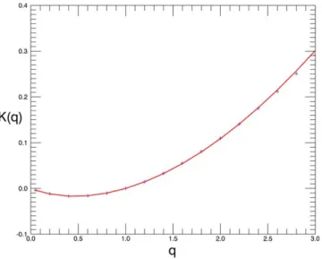
Figure 6.The plot shows an example of the moment scaling functionK(q) (for the EO data from English Channel from the October 2011). The points in the plot were calculated from the slopes of the different statistical moments and the full line shows the UM fit.
model. Figures 2 and 3 show that the model fluctuations scale with a steeper profile than the EO fluctua-tions. Figure 2 further shows that the EO data fluctuations remain seasonally almost unchanged, whereas the model fluctuations depend strongly on the seasonality. The EO data fluctuations are in general larger, with the exception of the summer period in the Irish Sea. The fluxes scaling (Figures 4 and 5) show signifi-cant differences in the energy input scalesLh(see the equation (24)) for the EO data and for the FVCOM model data. The EO data outer scale lies in the range of 1002300km(Figure 4), whereas the model outer scale is always larger than 500 km, with some values larger than 1000 km (Figure 5). The FVCOM model fluxes have steeper slopes than the EO fluxes, which indicates that the model dissipates energy at a higher rate than is observed in the EO data.
The universal multifractal (UM) fit (see the equation (7)) of the moment scaling functionK(q) had relative error
<5% and in most of the cases the error was around 1%. The moment scaling functionK(q) for the English Channel and the October 2011 data is shown in Figure 6. The UM parameters were calculated for both EO and FVCOM data. The annual ensemble averages of the values of theH;C1, andaparameters are shown
in Table 1. The table shows a consistent difference between the FVCOM model and EO UM parameters: the model parameterC1;H values are larger than theC1;H values of the EO data (see Table 1), whereas the
opposite is true for theaparameter. The correlation between the EO and the FVCOM multifractal parameters was relatively low, the Pearson coefficient was between 0.2 and 0.65, with larger values in the English Channel.
The models were compared with the EO data using three standard metrics: correlation coefficient, root-mean square error, and average error. In addition to that the two newly defined metrics UM1
(equation (11)) and UM2 were used. To use the UM1 and UM2 metrics the cutoff moments qD were
determined as qD5. The five metrics are compared in Figure 7 (Irish Sea) and Figure 8 (English Channel). In the Irish Sea region (Fig-ure 7) the three standard metrics (correlation coefficient, root-mean square error and average error) are mutually consistent and show a par-ticularly poor match between the EO and the FVCOM data in the final months of the year. This is because the model has a tendency to over-heat the upper ocean layer (the
mean FVCOM SST was 1–28 larger
than the EO SST). This tendency can be to some extent observed in the increase of UM2 values, but is not
shown by theUM1 metric (see Figure
7). This is an interesting example
showing that pixel-by-pixel based
comparisons (R, root-mean square error, average error) and structural comparisons (UM1;UM2) can lead to
very different results. In the English Channel (Figure 8), the picture is quite different, the values of all the
Table 1.TheH;C1, andaFIF Model Parameters Averaged Through the 2011 Year Overpasses
a
Parameter EO Irish FVCOM Irish EO English FVCOM English
hHi 0.557 0.651 0.655 0.839
hC1i 0.091 0.136 0.114 0.204
hai 1.721 1.598 1.67 1.485
a
The table compares both EO and FVCOM parameter values in both regions (Irish Sea and English Channel).
Figure 7.Comparison of different metrics for the Irish Sea region over 2011: (red) correlation coefficient, (blue) root mean square error, (green) absolute value taken from the average error, (yellow) theUM1metric comparing the overall size of fluc-tuations (the metric is defined by the equation (11)), (pink) theUM2metric com-paring the scaling profiles. The values of the root mean square error and the average error are in C, the remaining metrics are dimensionless.
metrics, change relatively little with time (except of fluctuations in UM2),
preserving the same seasonal profile. To get a better insight into the typical range of values ofUM1 andUM2, it is
interesting to analyze how the scaling properties measured through UM1;U M2evolve as one introduces noise into
the data with some known properties. Gaussian noise with changing variance was redistributed across the data set, where the variance of the noise was correlated to the field value. Figure 9 compares the two data sets, the data set with the noise and the original data set without the noise, for different noise amplitudes. Figure 9 shows the values of the UM1;UM2 metrics as a
function of the noise amplitude mea-sured by the root mean square error. Let us say that the second data set matches well the first data set, if the value of the root mean square error is bounded by 0:4C, which corresponds to the noise with variance about half of the natural variance of the data. Figure 9 then shows that theUM1andUM2values are bounded roughly
byUM11 andUM26. As seen from the Figures 7 and 8, the FVCOM model fulfills this bound for theUM2
metric, but not for theUM1metric. This suggests that the model captures well the overall field dynamics (data
structural scaling properties), but poorly represents the outer scale of the energy inputLh(which was already
dis-cussed in the previous paragraph) and potentially also the overall size of the SST fluctuations.
4. Discussion
The selection of nighttime data minimized the effect of the upper layer stratification on the data scaling. Despite that, the steeper slopes observed in the model data scaling can be at least partly explained by the relative thick-ness of the upper oceanic layer consid-ered by the FVCOM model. Stratification decreases the horizontal variability on smaller scales and therefore tilts the scal-ing slope towards steeper angles. The seasonal change in stratification can also explain the matching slopes of the EO and FVCOM fluctuations in the winter season (Figures 2 and 3) and the season-al variability in model fluctuations scseason-al- scal-ing (Figure 2). To explicitly confirm the hypothesis of the effect of stratification on the slope of the scaling, we split the English Channel region in Figure 1 into stratified (west) and mixed (east) regions [Pingree and Griffiths, 1978;Simpson and Bowers, 1981]. The scaling analysis in each of these two parts was then able to confirm the connection between stratification and the slope of the model data scaling.
Figure 8.Comparison of different metrics for the English Channel region over 2011: (red) correlation coefficient, (blue) root mean square error, (green) absolute value taken from the average error, (yellow) theUM1metric comparing the overall size of fluctuations (the metric is defined by the equation (11)), (pink) theUM2 metric comparing the scaling profiles. The values of the root mean square error and the average error are in degree Celsius, the remaining metrics are dimensionless.
Figure 9.The figure shows theUM1(red) andUM2(green) values as a function of data-correlated Gaussian noise with the amplitude measured by the root-mean square error (RMS).
It was observed that the FVCOM model overheated the upper layer in the Irish Sea region. This explains why the metrics values in the Irish Sea region (see Figure 7) evolve relatively rapidly with time, especially when compared to the stationary situation in the English Channel region (Figure 8). The overheating is also responsible for the FVCOM fluctuations being larger than the EO fluctuations during summer and vice versa in winter (visible in the scaling analysis).
The scaling analysis is an important indicator of dominant dynamical drivers shaping the field distributions [Skakala and Smyth, 2015]. One expects turbulent eddies to be one of the main factors behind the SST scale correlations. Another important factor in the shelf seas is the overall shape of the basin described through the bathymetry scaling exponents. As previously observed [Skakala and Smyth, 2015], the bathymetry scal-ing profile can have a significant impact on the scalscal-ing profile of the fields. Furthermore, in the EO overpass imagery data, tidal currents (largely shaped by the bathymetry) can play a significant role in driving the field distributions. The bathymetryHscaling exponent is larger in the English Channel region (H50.526) than in the Irish Sea (H50.302), and this could explain larger values of the EO dataH parameter in the English Channel, when compared to the Irish Sea region.
Unfortunately, the theoretical predictions for the large scale (>1 km) oceanic turbulence are ambiguous. There is no agreement in the literature if and how the effective two-dimensionality of the ocean at large scales (horizontal dimensions much larger than the vertical dimension) modifies the 3D turbulent model. This question is especially relevant in the shallow shelf seas (in our case mostly<100m). It has been sug-gested that the scaling exponents in the horizontal will remain the same as in case of 3D turbulence [ Love-joy and Schertzer, 2010], however, elsewhere [Currie and Roff, 2006], it is suggested that the two-dimensionality of the problem determines the value of theHexponent, which can lie anywhere between
H50.33 andH51 (H51 being the ideal 2D turbulence value). Here it has been observed that the EO data scaling exponentsH;C1, anda(from Table 1) do not deviate too significantly from the SST scaling
expo-nents observed on smaller scales inLovejoy et al. [2001b]. Particularly, theaparameter values from Table 1 are within the predictions ofLovejoy et al. [2001b]: a51:760:05. The model FIF parameters show larger deviations than the EO FIF parameters, but again, this can be explained by the stratification of the upper model layer.
5. Summary
The main purpose of this paper was to define two novel model skill evaluation metrics based on the univer-sal scaling properties. Those metrics are scale-free and lead to an interesting structural comparison of the EO and the model data sets. Their particular advantage over the presently used metrics lies in their connec-tion with the dominant dynamical drivers behind the field distribuconnec-tions. These metrics were applied to the FVCOM model in the shelf seas around the south-west of the UK: the paper attempts a comprehensive anal-ysis of the model performance. Some quality bounds were estimated for the novel metrics and it was shown that the FVCOM model captures most of the dynamical features of the EO data, but it overestimates the outer scale of the energy inputLh, which leads to some discrepancies between the EO and the model data scaling. The two metrics already provide us with significant part of the information about how the model represents field dynamics. At present there is, however, still relatively large ambiguity in how the field dynamics maps into the multifractal scaling. To fully exploit the information carried by these metrics, the future research goal is to use models to obtain a more precise map between oceanographic drivers and the three-dimensional universal multifractal parameter space.
References
Allen, J. I., and P. J. Somerfeld (2009), A multivariate approach to model skill assessment,J. Mar. Syst. 76, 83–94.
Adams, T. P., K. Black, C. MacIntyre, and R. Dean (2012), Connectivity modelling and network analysis of sea lice infection in Loch Fyne, west coast of Scotland,Aquaculture Environ. Interact.,3, 51–63.
Adams, T. P., D. Aleynik, and M. T. Burrows (2014), Larval dispersal of intertidal organisms and the influence of coastline geography, Ecogra-phy,37, 698–710.
Allen, J. I., P. J. Somerfeld, and F. J. Gilbert (2007a), Quantifying uncertainty in high resolution coupled hydrodinamic-ecosystem models,J. Mar. Syst. 64, 3–14.
Allen, J. I., J. T. Holt, J. Blackford, and R. Proctor (2007b), Error quantification of a high-resolution coupled hydrodinamic-ecosystem coastal-ocean model: part 2. Chlorophyll-a, nutrients and SPM,J. Mar. Syst. 68(3–4), 381–404.
Acknowledgments
We would like to thank the NERC Earth Observation Data Acquisition and Analysis Service (NEODAAS) at the Plymouth Marine Laboratory for preparing all the EO data for the analysis. The AVHRR satellite single overpass imagery can be obtained free from NEODAAS (https://www.neodaas. ac.uk). The bathymetry data were obtained from Liverpool Coastal Observatory (POLCOMS high resolution continental shelf model). They can be downloaded from http:// www.nodc.ac.uk/products/external_ products/celtic_seas/and http://www. gebco.net/. This work was partially supported by the UK Energy Research Centre (UKERC) Energy & Environment Phase II project and NERC/DEFRA FLOWBEC (NE/J004332/1). FVCOM was run on the NERC HPC facility (ARCHER). Surface forcing data for FVCOM were obtained from the National Centers for Environmental Prediction and Department of Energy Atmospheric Model Intercomparison Project (NCEP-DOE AMIP-II) Reanalysis-2 data. They can be obtained from http://www.esrl. noaa.gov/psd/data/gridded/data.ncep. reanalysis2.html. River temperature data for England were obtained from the Environment Agency Freshwater River Temperature Archive. These data can be obtained upon request from https://data.gov.uk/dataset/surface- water-temperature-archive-up-to-20071. River discharges were obtained from the E-HYPE European catchment model [Donnelly et al., 2012]. They can be obtained upon request from http:// hypeweb.smhi.se/europehype/.
Allen, J. I., T. J. Smyth, J. R. Siddorn, and M. Holt (2008), How well can we forecast high biomass algal bloom events in a eutrophic coastal sea?,Harmful Algae,8, 70–76.
Bak, P., C. Tang, and K. Wiesenfeld (1987), Self-organized criticality: An explanation of 1=fnoise,Phys. Rev. Lett.,59, 381–384.
Blackford, J. C., R. Torres, P. Cazaneve, and Y. Artioli (2013), Modelling dispersion of CO2plumes in sea water as an aid to monitoring and understanding ecological impact,Energy Proc.,37, 3379–3386.
Cazenave, P. W., R. Torres, and J. I. Allen (2016), Unstructured grid modelling of offshore wind farm impacts on seasonally stratified shelf seas,Prog. Oceanogr.,145, 25–41.
Chen, C., H. Liu, and R. C. Beardsley (2003), An unstructured grid, finite-volume, three-dimensional, primitive equations ocean model: Appli-cation to coastal ocean and estuaries,J. Atmos. Ocean Tech.,20, 159–186.
Chen C., H. Huang, R. C. Beardsley, H. Liu, Q. Xu, and G. Cowles (2007), A finite volume numerical approach for coastal ocean circulation studies: Comparisons with finite difference models,J. Geophys. Res.,112, C03018, doi:10.1029/2006JC003485.
Currie, W. J. S., and J. C. Roff (2006), Plankton are not passive tracers: Plankton in a turbulent environment,J. Geophys. Res.,111, C05S07, doi:10.1029/2005JC002967.
de Montera, L., M. Jouini, S. Verrier, S. Thiria, and M. Crepon (2011), Multifractal analysis of oceanic chlorophyll maps remotely sensed from space,Ocean Sci.,7, 219–229.
Doney, S. C., I. Limaa, J. K. Mooreb, K. Lindsayc, M. J. Behrenfeldd, T. K. Westberryd, N. Mahowalde, D. M. Glovera, and T. Takahashif (2008), Skill metrics for confronting global upper ocean ecosystem-biogeochemistry models against field and remote sensing data,J. Mar. Syst.,76, 95–112.
Donnelly, C., J. Rosberg, and K. Isberg (2012), A validation of river routing networks for catchment modelling from small to large scales,
Hydrol. Res.,44, 917–925.
Egbert, G. D., and S. Y. Erofeeva (2002), Efficient inverse modeling of barotropic ocean tides,J. Atmos. Oceanic Technol.,19, 183–204.
Egbert, G. D., A. F. Bennett, and M. G. G. Foreman (1994), TOPEX/POSEIDON tides estimated using a global inverse model,J. Geophys. Res.,
99, 24,821–24,852.
Gagnon, J. S., S. Lovejoy, and D. Schertzer (2006), Multifractal earth topography,Nonlin. Processes Geophys.,13, 541–570.
Gurvitch, A. S., and A. M. Yaglom (1967), Breakdown of eddies and probability distributions for small-scale turbulence,Phys. Fluids,10, 59– 65.
Harte, D. (2001),Multifractals: Theory and Applications, Chapman and Hall, N. Y.
Huang, H. (2011), Finite volume coastal ocean model (FVCOM) 3D hydrodynamic model comparison,Tech. Rep., La. State Univ., report num-ber: 0904830891, The Portal to Texas History, UNT Libraries, Baton Rouge, La.
Jolliff, J. K., J. C. Kindleb, I. Shulmanb, B. Pentab, M. A. M. Friedrichsc, R. Helberb, and R. A. Arnoneb (2009), Summary diagrams for coupled hydrodynamic-ecosystem model skill assessment,J. Mar. Syst. 76, 64–82.
Kohonen, T. (2000),Self-Organizing Maps, 3rd ed., 528 pp., Springer, Berlin, Germany.
Kolmogorov, A. N. (1941), Local structure of turbulence in an incompressible liquid for very large Reynolds numbers,Proc. Acad. Sci. URSS,
30, 299–303.
Lavalee, D., Lovejoy, S., Schertzer, D., and Ladoy, P. (1993), Nonlinear variability and landscape topography: Analysis and simulation, in Frac-tals in Geography, edited by L. deCola and N. Lam, pp. 171–205, Prentice Hall, N. J.
Lovejoy, S. (2014), A voyage through scales, a missing quadrillion and why the climate is not what you expect,Clim. Dyn.,44, 3187–3210. Lovejoy, S., and D. Schertzer (2010), Towards a new synthesis for atmospheric dynamics: Space-time cascades,Atmos. Res.,96, 1–52. Lovejoy, S., and D. Schertzer (2013),The Weather and Climate: Emergent Laws and Multifractal Cascades, Cambridge Univ. Press, Cambridge,
U. K.
Lovejoy, S., D. Schertzer, and J. D. Stanway (2001a), Direct evidence of multifractal atmospheric cascades from planetary scales down to 1 km,Phys. Rev. Lett.,86(22), 5200.
Lovejoy, S., W. J. S. Currie, Y. Tessier, M. R. Claereboudt, E. Bourget, J. C. Roff, and D. Schertzer (2001b), Universal multifractals and ocean patchiness: phytoplankton, physical fields and coastal heterogeneity,J. Plankton Res.,23(2), 117–141.
Mandelbrot, B. (1974), Intermittent turbulence in self-similar cascades: Divergence of high moments and dimension of the carrier,J. Fluid Mech.,62, 331–358.
Mandelbrot, B. (1982),The Fractal Geometry of Nature, W. H. Freeman and Co., N. Y. Mandelbrot, B. (1997),Fractals and Scaling in Finance, Springer, N. Y.
Novikov, E. A., and R. Stewart (1964), Intermittency of turbulence and spectrum of fluctuations in energy dissipation,Izv. Akad. Nauk. SSSR, Ser. Geofiz.,3, 408–412.
Obukhov, A. (1949), Structure of the temperature field in a turbulent flow,Izv. Akad. Nauk. SSSR,13, 55–69.
Orr, H. G., et al. (2010), Changing water temperatures: A surface water archive for England and Wales, inRole of Hydrology in Managing Con-sequences of a Changing Global Environment, edited by C. Kirby, Br. Hydrol. Soc, U. K.
Pingree, R. D., and D. K. Griffiths (1978), Tidal fronts on the shelf seas around the British Isles,J. Geophys. Res.,83, 4615–4622.
Radic, V., and G. Clarke (2011), Evaluation of IPCC models’ performance in simpulating late twentieth-century climatologies and weather patterns over North America,J. Clim.,24, 5257–5274.
Richardson, L. F. (1922),Weather Prediction by Numerical Processes, Cambridge Univ. Press, Cambridge, U. K.
Saux Picart, S., Butenschon, M., and J. D. Shutler (2012), Wavelett-based spatial comparison technique for analysing and evaluating two-dimensional geophysical model fields,Geosci. Model Dev.,5, 223–230.
Schertzer, D., and S. Lovejoy (1987), Physical modelling and analysis of rain and clouds by anisotropic scaling multiplicative processes,J. Geophys. Res.,92, 9693–9714, doi:10.1029/JD092iD08p09693.
Schertzer, D., and S. Lovejoy (1988), Multifractal simulations and analysis of clouds by multiplicative processes,Atmos. Res.,21, 337–361. Schertzer, D., and S. Lovejoy (1997), Universal multifractals do exist!,J. Appl. Meteorol.,36, 1296–1303.
Schertzer, D., and S. Lovejoy (2011), Multifractals, generalized scale invariance and complexity in geophysics,Int. J. Bifurcation Chaos,
21(12), 3417–3456.
Schmitt, F., D. Schertzer, S. Lovejoy, and Y. Brunet (1993), Estimation of universal for atmospheric turbulent multifractal indices velocity fields,Fractals,01, 568.
Seuront, L., and Y. Lagadeuc (1997), Characterization of space-time variability in stratified and mixed coastal waters (baie des Chaleurs, Quebec, Canada): Application to fractal theory,Mar. Ecol. Prog. Ser.,259, 81–85.
Seuront, L., and F. G. Schmitt (2005a), Multiscaling statistical procedures for the exploration of biophysical couplings in intermittent turbu-lence; Part I. Theory,Deep Sea Res., Part II,52, 1308–1324.
Seuront, L., and F. G. Schmitt (2005b), Multiscaling statistical procedures for the exploration of biophysical couplings in intermittent turbu-lence; Part II. Applications,Deep Sea Res., Part II,52, 1325–1343.
Seuront, L., F. Schmitt, Y. Lagadeuc, D. Schertzer, S. Lovejoy, and S. Frontier (1996a), Multifractal analysis of phytoplankton biomass and temperature in the ocean,Geophys. Res. Lett.,23(24), 3591–3594.
Seuront, L. et al. (1996b), Multifractal intermittency of Eulerian and Lagrangian turbulence of ocean temperature and plankton fields, Non-linear Processes Geophys.,3, 236–246.
Seuront, L., et al. (1999), Universal multifractal analysis as a tool to characterize multiscale intermittent patterns: Example of phytoplankton distribution in turbulent coastal waters,J. Plankton Res.,21, 877–922.
Seuront, L., H. Yamazaki, and F. Schmitt (2005), Intermittency, inMarine Turbulence, edited by H. Baumert, J. Simpson, and J. Sundermann, pp. 66–79, Cambridge Univ. Press, Cambridge, U. K.
Simpson, J. H., and D. Bowers (1981), Models of stratification and frontal movement in shelf seas,Deep Sea Res., Part A,28, 727–738. Shutler, J. D., T. J. Smytha, S. Saux-Picarta, S. L. Wakelinb, P. Hyderc, P. Orekhova, M. G. Granta, G. H. Tilstonea, and J. I. Allen (2011),
Evaluat-ing the ability of a hydrodynamic ecosystem model to capture inter- and intra-annual spatial characteristics of chlorophyll-a in the north east Atlantic,J. Mar. Syst.,88, 169–182.
Skakala, J., and T. J. Smyth (2015), Complex coastal fields can be described by universal multifractals,J. Geophys. Res.,120, 6253–6265, doi: 10.1002/2015JC011111.
Smagorinsky, J. (1963), General circulation experiments with the primitive equations I: The basic experiment,Mon. Weather Rev.,91, 99– 164.
Stow, C. A., J. Jolliffb, D. J. McGillicuddy Jr., S. C. Doneyc, J. I. Allend, M. A. M. Friedrichse, K. A. Rosef, and P. Wallheadg (2009), Skill assess-ment for coupled biological/physical models of marine systems,J. Mar. Syst.,76, 4–15.
Taylor, K. E. (2001), Summarizing multiple aspects of model performance in a single diagram,J. Geophys. Res.,106(7), 7183–7192. Torres, R., and R. J. Uncles (2011),Modeling of Estuarine and Coastal Waters, vol. 2, Elsevier, Perth, Australia.
Umlauf, L., and H. Burhcard (2005), Second-order turbulence closure models for geophysical boundary layers. A review of recent work,
Cont. Shelf Res.,25, 795–827.
Yaglom, A. M. (1966), The influence on the fluctuation in energy dissipation on the shape of turbulent characteristics in the inertial interval,
Sov. Phys. Dokl.,2, 26–30.
Yang, Z., and K. Tarang (2008), Modeling of salt intrusion, intertidal mixing, and circulation in a braided estuary,J. Coastal Res.,52, 171–180. Yang, Z., T. Wang, and A. E. Copping (2013), Modeling tidal stream energy extraction and its effects on transport processes in a tidal
chan-nel and bay system using a three-dimensional coastal ocean model,Renewable Energy,50, 605–613.
Zheng, L., and R. H. Weisberg (2012), Modeling the west Florida coastal ocean by downscaling from the deep ocean, across the continental shelf and into the estuaries,Ocean Model.,48, 10–29.