Aeroelastic Analysis of a Typical Section using Euler and Navier-Stokes Mesh-less Method

Sharif University of Technology

Transactions B: Mechanical Engineering www.scientiairanica.com

Aeroelastic analysis of a typical section using Euler and

Navier-Stokes mesh-less method

S. Sattarzadeh, A. Jahangirian

_{and H. Shahverdi}

Department of Aerospace Engineering, Amirkabir University of Technology, 424 Hafez Avenue, Tehran, P.O. Box 15875-4413, Iran. Received 23 April 2014; received in revised form 2 August 2014; accepted 13 April 2015

KEYWORDS Aeroelastic instability; Compressible ow; Flutter speed; Mesh-less method; Navier-Stokes equations; Transonic ow.

Abstract. The main aim of this paper is to develop an ecient aeroelastic tool for predicting the utter speed of a typical section in transonic regime. An implicit mesh-less method, based on Euler and Navier-Stokes equations, is conducted to simulate the transonic uid ow around an airfoil. This technique is applied directly to the dierential form of the aerodynamic governing equations and the time integration is carried out using a dual-time implicit time discretization scheme. The capabilities of the ow solution method are demonstrated by ow computations around NACA0012 airfoil under dierent ow conditions. For structural dynamics simulation, a typical section model with pitching and plunging motion capability is considered. Finally, the aeroelastic analysis of the 2D model is performed by the consecutive simulation of both structural and aerodynamic domains. Also, the eect of viscosity and time interval choice between two structural and aerodynamic solvers on utter instability is studied. A comparison between the obtained results and those available in the literature shows the good accuracy of the present method. © 2016 Sharif University of Technology. All rights reserved.

1. Introduction

There is no escaping the fact that aeroelastic stability investigations play an important role in the design-ing process of an air vehicle. The most performed activities and research in the aeroelastic eld have been determination of critical utter speed. In this regard, nding a suitable and powerful method for solving structural and uid ow elds has always been an attractive subject for researchers [1,2]. Specically, from a uid computational aspect, some well-known analytical models, such as Theodorsen's theory for unsteady subsonic incompressible ow and the piston theory for supersonic applications, are reachable (of course with some limitations) [3]. Moreover, the Computational Fluid Dynamics (CFD) method can be

*. Corresponding author. Tel.: +98 21 64543223

E-mail addresses: [email protected] (S. Sattarzadeh); [email protected] (A. Jahangirian); h [email protected] (H. Shahverdi)

put into use to study the complex phenomena of a uid ow (e.g. ow separation, compressibility, shock, etc.). Using these methods may increase solution complexity and computational eort, and, thus, solution of an especial case, such as a transonic ow regime, with a suitable tool, is an important challenge in aeroelastic analysis. Transonic aeroelasticity is more complex in comparison with subsonic and supersonic regimes due to the existence of shock waves across the airfoil. In these regimes, the uid ow equations can be used in the linear form, which could be incorporated into aeroelastic equations. However, transonic ow has a nonlinear nature that is not easy to be solved with the same techniques. One way to overcome these diculties is to use numerical methods (CFD) which may be implemented through time-marching schemes. Finite element or nite volume methods are ex-tensively applied to address the computational aeroe-lasticity eld problems [4-6]. However, most of these studies have some restrictions in transonic ow. The rst aeroelastic study in the transonic regime was

performed by Edwards et al. [2]. In this paper, a nonlinear time-marching aeroelastic model was solved using Transonic Small Disturbance (TSD). Bendiksen and Kousen achieved the utter boundaries for a NACA 64A010 airfoil using an explicit method based on the convolution integral. They found that the large-amplitude limit cycles could be achieved in unsteady motion [7]. Lee studied the eect of viscosity using the Finite Volume (FV) method [8]. Kholodar et al. [9] applied a novel Harmonic Balance (HB) technique to solve the utter boundary in the presence of Euler equations. In other work by Thomas et al. [10,11], this method was developed for N-S equations to predict utter velocity. The eect of viscosity on utter velocity in the transonic regime, based on the HB method, was investigated by Schwarz et al. [12].

Guruswamy [13] attained acceptable results using dierent equations for 2D and 3D geometries, including vertical ow. To capture valid results in these methods, a rened mesh is required. Indeed, the problem of these methods will be initiated when the complexity of the model and its operational conditions are increased.

Compared to mesh-based methods, mesh-less methods have some advantages. For example, the main problem of Computational Fluid Dynamics (CFD) in mesh-based methods is their diculties in generation of a practical mesh [14]. But, in mesh-less methods, only computational points (instead of elements) are used in the solution process. One of the major disadvantages of all mesh-based methods (especially in aero-elastic analysis) is their diculty in the solution of unsteady ow because of element deformation. This obstacle could be resolved using mesh-less methods, which employ computational points that are easily replaced and moved in comparison with mesh-based algorithms. This privilege can be useful especially in unsteady conditions (because of a large number of time steps in unsteady computations). These advantages encourage the use of mesh-less method in aero-elastic applications. Dierent mesh-less methods have been presented in the literature [15,16]. A very ecient implicit mesh-less method is applied to solve steady compressible ows by Jahangirian and Hashemi [17]. In that paper, the least square method, based on the Taylor series, was applied to calculate the derivatives. The results indicated that the computational time is decreased by 50% in comparison with the similar Control Volume (CV) method using the same point distribution [18]. In this paper, implicit and explicit methods were developed to solve unsteady stationary ows. The unsteady mesh-less method, based on point replacement, has been provided by Wang et al. [19] and Ortega et al. [20]. In another work, Wang et al. [21] used Delaunay triangle principles to solve unsteady ow.

Several mesh-less methods have been applied for

uid-solid interaction problems [22-25]. For instance, Hu et al. [22] applied the Pure Particle Method (PPM) to complex geometries, along with large deformation capability. In another work, a staggered algorithm, based on the mesh-less method, has been extended for uid-structural interaction [23]. However, only a few works have been performed based on the least square method.

The main objective of the present work is to further extend the application of the least square mesh-less method to aeroelastic moving boundary unsteady problems under transonic ow conditions. At the rst stage, the ability of the ow solution method is demonstrated. It is shown that the convergence rate of this method is higher than the similar Control Volume (CV) method with the same discretization and initial data [18]. In the next step, the ability of the method is shown regarding the solution of unsteady ow. Then, the provided computational aerodynamic model is incorporated into the system of aeroelastic equations of a typical section model to perform aeroelastic analysis. Also, the eect of viscosity on utter instability is studied.

2. Computational models 2.1. Aerodynamic model

The uid ow around a moving, two-dimensional airfoil is governed by Navier-Stokes (N-S) equations, which can be written in the dierential form as [17]:

@w

@t + wr ws + @fI @x + @gI @y

= Ma_Re1

1 @fV @x + @gV @y ; (1) where: w = 0 B B @ u v E 1 C C

A ; ws=

xt

yt

fI ₌

0 B B @

U uU + P

vU EU + P u

1 C C A ;

gl₌

0 B B @ V uV vV + P EV + P v

1 C C

A ; fV = 0 B B @ 0 xx xy

uxx+ vxy qx

1 C C A ;

gV ₌

0 B B @ 0 xy yy

uxy+ vyy qy

1 C C

A : (2)

U and V represent the x and y components of relative velocity and are evaluated as:

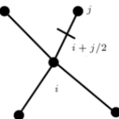
Figure 1. A sample point and its neighbors.

For a perfect gas, the following equation can be written as:

P = ( 1)

E (u2+ v2) 2

: (4)

In this study, for applying the mesh-less method, equations are used in a conservation form. In this method, the dierential form of governing equations is implemented, and a least-square approximation is used to calculate the derivatives [26]. According to Figure 1, Ci is the set of computational points,

which are neighbors for point i, and the value of any parameter, , is dened at the mid-point between two adjacent points [27]. The amount of function ij is

assumed to change linearly along line ij. Using Taylor's formula for point i and its neighboring points, the following equation is achieved [17]:

@ @x

xij+

@ @y

yij= ij; xij= xj xi;

yij = yj yi; ij = j i: (5)

Similar equations are achieved for all cloud points which are neighbors with point i by considering an arbitrary weighting factor, !i. This may result in the

following matrix for point i [26]: 0

@!i1 xi1 !i1 yi1 !imxim !imyim

1 A

2 4

@ @xji @ @yji

3 5 =

2

4!i1 i1 !imim

3 5 ; !ij =_d1

ij: (6)

By considering Eq. (5) and using the least-squares method, the derivatives of each parameter can be estimated as follows [26]:

@ @x i= m X j=1

aijij; @_@y

i= m X j=1

bijij: (7)

The coecients in Eq. (7) can be computed through solving Eq. (6) [16]:

aij=

!ijxijPm_k=1!ikyik2 !ijyijPm_k=1!ikxikyik

P_m

k=1!ikx2ij

P_m

k=1!ikyik2 (

P_m

k=1!ikxikyik)2

bij =

!ijyijPmk=1!ikx2ik !ijxijPmk=1!ikxikyik

P_m

k=1!ikx2ijPmk=1!ikyik2 (

P_m

k=1!ikxikyik)2

: (8) To achieve a semi-discrete form of the Navier-Stokes equations (Eq. (1)) at point i, using Eq. (7), the following equation is obtained [16]:

2 4@wi

@t + wi 0 @Xm

j=1

aijxt;ij+ m

X

j=1

bijyt;ij

1 A 3 5 + 2 4Xm

j=1

aijfijI + m

X

j=1

bijgIij

3 5

=Ma_Re1

1

2 4Xm

j=1

aijfijV + m

X

j=1

bijgVij

3 5 ;

i = 1:::N: (9)

In this equation, fij and gij are:

fij = fj fi; gij = gj gi: (10)

By dening H = aF + bG (which is dened as ux in the direction of the least square coecients and is similar to ux which is calculated in the mesh-based methods [17]) in Eq. (9), the following equation can be achieved:

@wi

@t + wi _Xm

j=1

aijxt;ij+ m

X

j=1

bijyt;ij

+Xm

j=1

HI

ij= Ma_Re1 1

2 4Xm

j=1

HV ij

3 5 ;

Hij= Hj Hi: (11)

By applying the central dierence method to the Navier-Stokes equations, the following equation can be achieved:

@wi

@t + wi _Xm

j=1

aijxt;ij+ m

X

j=1

bijyt;ij

+ 2Xm

j=1

HI

i j+1=2=2Ma_Re1 1

2 4Xm

j=1

HV i j+1=2

3 5

Hj+1=2=Hi+ H₂ j: (12)

unstable results are achieved. In order to overcome this problem, stabilizing terms are used in Eq. (9) by adding damping terms. In this dissipation model, in order to prevent oscillations, especially in critical zones, an aggregation of the second and fourth dierences of conserved variables (W ) is added to Eq. (11) [17], which is denoted by the D symbol in the following relation:

@wi

@t + 2 _Xm

j=1

HI

i j+1=2 Ma_Re1 1 _Xm j=1 HV i j+1=2

Di= 0: (13)

These dissipation terms are dened by: Di=

r("(2)_{)rW r}2_("(4)_)r2_W i;

r("(2)_{)rW =}Xn j=1

h ("(2)₎

i;j=2(Wj Wi)

i ;

r2_{W =}Xn j=1

(Wj Wi); (14)

where "(2) _{and "}(4) _{can be formulated as:}

"(2)_ij = k2vij;

"4

ij = max

0; k4 "(2)ij

;

vij =jP_jPj Pij

j+ Pij: (15)

The values of constant k2 and k4 are in the range

0 < k2 < 1 and 2561 < k4 < 321 [28]. Eq. (11) is

applied to each node in the computational domain and a set of ordinary dierential equations are obtained as follows [28]:

@Wi

@t + R(Wi) = 0;

Ri(W ) =Wi

_Xm

j=1

aijxt;ij+ m

X

j=1

bijyt;ij

+Xm

j=1

HI

ij Ma_Re1 1

2 4Xm

j=1

HV ij

3 5 Di;

dW

dt + R(Win+1) = 0: (16)

An implicit time discretization is applied in Eq. (16), which can be written as [17]:

@wn+1 i

@t + Ri(wn+1) = 0: (17)

In this equation, the superscript n+1 is applied for time level (n + 1). For d

dt, by using the implicit backward

dierence, by considering the order of accuracy of k, the following equation is achieved:

d dt 1 t k X q=1 1

q[ ]q; (18) where:

wn+1_{= w}n+1 _wn_{: (19)}

Considering the second order accuracy, the following equation can be obtained:

3wn+1 i

2ti

4wn i

2ti +

wn 1 i

2ti + Ri(w

n+1_{) = 0; (20)}

where wn+1_i is nonlinear and, so, cannot be solved by analytical methods. To overcome this problem, a new residual, R_{, is dened and referred to the unsteady}

residual:

R

i(wn+1) =3w n+1 i

2ti

4wn i

2ti +

wn 1 i

2ti

+ wn+1 i

_Xm

j=1

aijxt;ij+ m

X

j=1

bijyt;ij

+Xm

j=1

HI

ij(wn+1)

Ma1

Re1

2 4Xm

j=1

HV

ij(wn+1)

3 5

Di(wn+1): (21)

This equation can be used to solve steady-state prob-lems by considering a new pseudo time ().

@wn+1 i

@ + Ri(wn+1) = 0: (22)

To solve the steady-state problem, one can have: @wn+1_i

@ = 0: (23)

By comparing two equations, we can have R

i(wn+1) =

0, which can be used to solve Eq. (24). By considering time marching methods, such as the Runge-Kutta method [23], the solution can be found.

In this research, implicit and explicit CFL numbers are assumed to be 100000 and 5, respec-tively [17,28]. To solve Euler and Navier-Stokes equations at a solid boundary, it is assumed that the

Figure 2. Schematic of boundary zone.

boundary is reective and impenetrable [17], which can lead to the following assumption for a solid boundary: un= 0; @u_@nt =0; @H_@n= 0; @_@n=0; @P_@n = 0:

(24) To achieve a better result, especially in the solid bound-ary region, the Ghost point method [17] is employed. In this method, some new points are added to improve the accuracy of the mesh-less method in the solid boundary (Figure 2). For the new points, the velocity components are calculated as the following:

ug= (uj 2 _xb); vg= (vj 2 _yb);

For viscous ow;

ug= uj 2jVnjnx; vg= vj 2jVnjny;

For inviscid ow: (25) Also, in the far eld, characteristic analysis based on Riemann invariants are exploited [17]. The points neighbouring stencils inside the boundary layer region and outside this area are shown in Figure 3.

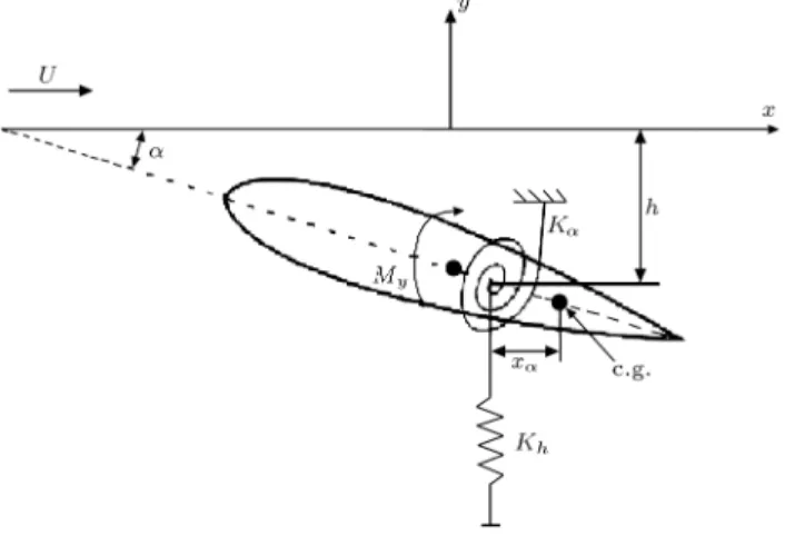
2.2. Structural model

A NACA 0012 airfoil section model with plunging and pitching motion has been considered as a two-dimensional test case of the structural model. As shown in Figure 4, the exibility of each degree of freedom has been shown using two discretized spring models.

Figure 3. Neighboring stencils.

Figure 4. Typical section model.

The structural dynamics equations of motion can be written as follows [3]:

mh + S + Khh = Qh;

Sh + I + K = Q: (26)

Since the aerodynamic equations are developed in dimensionless form, it is better to use the non-dimensional form of the structural equations. Thus, they can be written as [3]:

h + 1

2x + 4 !2

r

~u2h = cl ; (27)

xh + 1₂r2 + 2r 2

~u2 =

4cm

; (28)

where h is dened by the following relation:

h = h_c; (29)

is dened as:

=b2

m : (30)

Also, !r can be explained as:

!r=_!!h

: (31)

Finally, the above equations, along with the aero-dynamic equations, could be incorporated into the framework of aero-elastic analysis.

2.3. Solution methodology

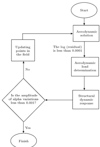
To perform elastic analysis, structural and aero-dynamic equations are solved sequentially. In this way, the unsteady aerodynamic loads are rstly determined using the mesh-less method for certain free-stream conditions. In the next step, these computed loads are

applied to the structural model and they are solved by a transient dynamic analysis. Then, the obtained results, including deformations (structural dynamic response) and induced velocities, are applied to the aerodynamic model in order to update its geometry and boundary conditions for the next unsteady solution. This process continues until the user dened end condition of the problem is met. In this situation, the solution is repeated until the dierence between the amplitudes of two successive picks of the alpha and displacement response become less than 0.001. For the aerodynamic solver, it is notable that at each time step, the average error should reach the level of less than 0.0001. It must be noted that for transient dynamic analysis, the 4th order Runge-Kutta scheme is used. The owchart of this aeroelastic solution algorithm is shown in Figure 5. Using the above mentioned methodology, an investigation is carried out about the eects of dierent parameters using the complete CFD-structural system.

3. Results

To validate the present method and show its capability for aeroelastic computations, several numerical inves-tigations are carried out which are explained in the following subsections.

Figure 5. The owchart of the aeroelastic analysis.

Figure 6. Point distribution around NACA0012 (viscous case).

3.1. Viscous case

To show the eect of viscosity and to show the ability of the method in comparison with the control volume, the rst case is considered with ow conditions of Ma = 0:8 and Re = 500. The generated point distribution around the airfoil is shown in Figure 6, which includes 13233 points in total, 72 points of which are located on the outer boundary and 364 nodes lie on the solid boundary. In this case, both Euler and Navier-Stokes solutions are obtained, and the related results are shown in Figures 7 and 8, respectively. It is notable that in this case, the amounts of dissipation terms, "(2)

and "(4)_{, are 0.5 and 0.015, respectively.}

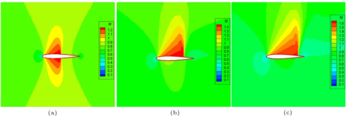
In these gures, Mach number contours for dif-ferent angles of attacks are shown. As illustrated, there are considerable dierences between the inviscid and viscous results, which clearly show the viscosity eect in this problem. Surface pressure distributions in dierent situations are shown in Figure 9. As is clear, viscous terms play an important role in shock involved problems. To show the ability of the method, the con-vergence rate and the pressure coecient distribution of the method at Ma = 0:8 and AOA=2.5 are compared with similar CV methods with the same discretization and the same initial data [18]. Figure 10(a) illustrates that good results are achieved in comparison with the CV method. The convergence history is shown in Figure 10(b). As is obvious, the mesh-less method has better convergence in comparison with the CV method. The computations are performed on a Dual core PC with 2.00 GHz speed. This benet can be more helpful in aeroelastic analysis, especially in saving CPU time.

3.2. Unsteady case

The next case is chosen to simulate the unsteady ow solution around an oscillating NACA0012 airfoil at

Figure 7. Mach contours around NACA0012 using Euler equations at Ma = 0:8: (a) AOA=0; (b) AOA=2.5; and (c) AOA=5.0.

Figure 8. Mach number contours around airfoil using N-S equations at Ma = 0:8: (a) AOA=0; (b) AOA=2.5; and (c) AOA=5.0.

Figure 9. Surface pressure distributions at dierent times at Ma = 0:8: a) AOA=0; b) AOA=2.5; and c) AOA=5.0.

Figure 10. (a) The pressure coecient distribution. (b) The convergence rate for NACA 0012. Ma = 0.8, AOA = 2.5, Re = 500

Figure 11. Point distribution model around NACA00012 airfoil.

Mach number of 0.8. The close-view of the point distribution around the airfoil is shown in Figure 11. The point cloud contains 6509 points, of which 275 points lie on the solid boundary. The outer boundary is located 10 chords away from the airfoil with 65 points on it. The point distribution is chosen the same as in the rst case. In this case, the periodic pitch angle can be considered as follows:

(t) = (m+ 0sin(!t)) ; (32)

where mand 0are equal to 0.00 and 1.0, respectively.

! can be calculated as follows: ! =2kU1

c : (33)

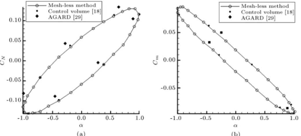
In this investigation, k is chosen as 0.1. Figure 12 shows normal force coecients and pitching moment coecients for inviscid ow. In this gure, the results are compared with CV numerical results from [18] and the experimental data of the AGARD [29]. As shown, good results are achieved in comparison with other reliable methods.

Table 1. Specications of typical section model. (kg/m3_{) 1.2255 M (kg) 19.6245} I (kg.m2_{) 4.1021 Kh (N/m) 1962.45518}

K (N.m/rad) 2563.8178 x 0.1

C = 2b (m) 1.8288 -0.2

3.3. Flutter study

The ability of the present method to predict aeroelastic instability is investigated by the utter analysis of a typical section. The structural and geometrical specications of the model are listed in Table 1.

To conduct aeroelastic analysis, rstly, the de-veloped unsteady Euler solver is utilized for uid computations in the coupled uid-structure simulation. The point cloud is considered the same as in the inviscid case. Table 2 shows the obtained utter velocity and utter frequency of this model in comparison with other reference data [30,31]. It must be noted that the mentioned reference data are obtained using an analytical aerodynamic model (Theodorsen's theory) to capture the utter speed. Also, for the velocity beyond this critical value, for example v = 0:3, some snap shots of the ow eld and structural response are presented in Figures 13 and 14. These gures reveal that both amplitude responses of the system increase in a rapidly progressive manner. Thus, the aeroelastic system behaves in an unstable fashion.

The other notable point is that by choosing an unsuitable time interval (t), numerical instability can occur. This can aect the results and an inap-propriate utter speed, which are predicted by the present method [32]. For example, by choosing v = 49 m/sec and two dierent time intervals, as shown in Figure 15, dierent results are achieved. As is obvious, in Figure 15(a), by choosing t = 0:000001, the amplitude response of the system increases, while in Figure 15(b), with the same initial data, and by choosing t = 0:0001, the utter is predicted. These

Figure 13. A few snap shots of the ow eld for v = 0:3 at (a) 1 min, (b) 2 min, (c) 3 min, (d) 4 min, (e) 4:30 min, and (f) 5 min.

Figure 14. (a) vs. time, and (b) h vs. time at v = 0:3. Table 2. Flutter speed of typical section model.

Present result Ref. [30] Ref. [31] Flutter velocity 49.164 m/sec 50.5968 m/sec 52.42 m/sec Flutter frequency 96.345 rad/sec 100.19 rad/sec 104.34 rad/sec

results show that a proper time interval should be chosen to prevent numerical instability.

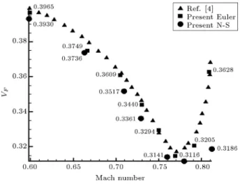
For investigation of the ability of the present method to analyze aeroelasticity under a compress-ibility eect, especically in the transonic regime, an aeroelastic analysis of the previous model, under dierent Mach numbers, is conducted, and the obtained results are shown in Figure 16. This gure shows that the present method, based on the Euler equation,

has good agreement with Ref. [4], and conrms the acceptable accuracy of the presented mesh-less method in aeroelastic computations. It must be noted that in Ref. [4], Euler equations are applied using interpolation techniques, such as kriging and Articial Neural Net-works (ANN), to predict utter speed in the transonic regime.

For comparing the results of dierent studies, the utter index (VF) is dened as:

Figure 15. The eect of time interval on utter speed predicting at (a) t = 0:000001, and (b) t = 0:0001.

Figure 16. VF vs. Mach number.

VF =p~u (34)

Figure 16 shows that the utter index decreases with increasing the Mach number until critical Mach num-ber. However, after this value, the utter index increases sharply with increasing Mach number. The transonic dip [33] can be seen in this gure, which is because of the compressibility eects [34]. Also, the obtained results show that considering the viscosity in aeroelastic computations has little eect on the stability results if the ight Mach number is less than critical. Thus, for this ight condition, the Euler equation can be considered to overcome numerical complexity [9]. For higher Mach number, the N-S curve dierences become large because, in this region, the viscous eect cannot be neglected. In this zone, the viscosity can replace the position of the shock, which has an important role to play in separation of the boundary layer. Thus, the utter index can be aected by boundary layer separation [34]. The dierences between the position of separations and shock waves in Euler and N-S equations after Ma = 0.76 creates enormous variations between the two results.

4. Conclusions

In this paper, a numerical aeroelastic model for a typical section (two-dimensional wing) via a mesh-less model is developed. For utilizing the time-marching technique, a dual-time implicit time discretization scheme was applied and the computational eciency was enhanced by adopting accelerating techniques. The obtained results showed the validity of the devel-oped solver for the uid ow computations in compari-son with available data. In addition, it was found that the time of convergence in this method is better than in the CV method. The ability of the method was shown by simulating the unsteady ow solution around an oscillating NACA0012 airfoil. Also, the capability of the present method to conduct aeroelastic analysis was shown using two dierent test cases in subsonic and compressible regimes (up to transonic regime). The results show the ability and accuracy of the present method to perform transonic aeroelastic analysis. Also, it has been shown that the viscosity eect can be neglected in transonic aeroelastic analysis when the ight Mach number is less than critical. It was shown that the choice of time interval has a signicant eect on the proper prediction of utter speed.

Nomenclature

u Velocity component in x direction v Velocity component in y direction U Relative velocity in x direction V Relative velocity in y direction un Normal velocity

ut Tangential velocity

xt Nodal velocity in x direction

yt Nodal velocity in y direction

Vv Nodal velocity

E Total energy

dij Distance between points i and j

aij Least square coecient in x direction

bij Least square coecient in y direction

D Articial dissipation Ma1 Mach number in far eld

Re1 Reynolds number in far eld

h Plunging motion h Dimensionless form of h m Mass of the airfoil c Chord length k Reduced frequency U1 Free-stream velocity

VF Flutter index

S Static mass unbalance

I Mass moment of inertia about the

elastic center

Kh plunge spring constant

K Pitch spring constant

Qh Lift force

Q Aerodynamic pitching moment about

the elastic center

~sij Unit vector between i and j

S Static mass unbalance

I Mass moment of inertia about the

elastic center

~u Dimensionless reduced velocity

r Dimensionless radius of gyration about

the elastic center

x A scale of distance between the center

of gravity and the elastic center vij Pressure sensor shock at any edges (ij)

"(2) _{Local adaptive coecients in critical}

zones

"(4) _{Local adaptive coecients in}

non-critical zones !i Weighting factor

Pitching angle m Mean angle

0 Oscillation amplitude

! Frequency of the system Non-dimensional mass Ratio of the specic heats

!r Ratio of uncoupled natural frequencies

!h Uncoupled plunge natural frequency

! Uncoupled pitch natural frequency

Density

r'_j+1=2 The average of gradients of any variable at midpoint

References

1. Garrick, I.E. and Reed, W.H. \Historical development of aircraft utter", Journal of Aircraft, 18(11), pp. 897-912 (1981).

2. Edwards, J.W., Bennett, R.J. and Seidel, D. \Time marching transonic utter solutions including angle of attack eects", AIAA Journal, 20(11), pp. 899-906 (1982).

3. Clark, R., Cox, D., Curtiss, H., Edwards, J., Hall, K., Peters, D., Scanlan, R., Simiu, E., Sisto, F., Strganac, T. and Dowell, E.H., A Modern Course in Aeroelasticity (Solid Mechanics and Its Applications), Springer, 4th Rev. Ed. (2004).

4. Timme, S., Rampurawala, A. and Badcock, K.J. \Ap-plying interpolation techniques to search for transonic aeroelastic instability: ANN vs kriging", The RAES Aerodynamics Conference, Bristol, United Kindom (2010).

5. Mariem, J.B. and Hamdi, M.A. \A new boundary nite element method for uid-structure interaction problems", Int. J. for Numerical Methods in Engineer-ing, 24(9), pp. 1251-1267 (1987).

6. Wang, X. and Bathe, K.J. \Displacement/pressure based mixed nite element formulations for acoustic uid-structure interaction problems", Int. J. for Nu-merical Methods in Engineering, 40 (11), pp. 2001-2017 (1997).

7. Kousen, K.A. and Bendiksen, O.O. \Nonlinear aspects of the transonic aeroelastic stability problem", Pre-sented at the AIAA/ASME/ASCE/AHS29th Struc-tures, Structural Dynamics, and Materials Confer-ence, Williamsburg, Virginia, DOI: 10.2514/6.1988-2306 (1988).

8. Lee, S. \Viscosity inuence on utter boundary and limit cycle oscillation in transonic regime", Journal of Fluid Science and Technology, 3(1) pp. 195-206 (2008).

9. Kholodar, D.B., Dowell, E.H. and Thomas, J.P. \Limit cycle oscillations of a typical section airfoil in transonic ow", Journal of Aircraft, 41(5), pp. 1067-1072 (2004).

10. Thomas, J.P., Dowell, E.H. and Hall, K.C. \Nonlinear inviscid aerodynamic eects on transonic divergence, utter and limit cycle oscillations", AIAA Journal, 40(4), pp. 638-646 (2002).

11. Thomas, J., Dowell, E. and Hall, K. \Modeling viscous transonic limit-cycle oscillation behavior using a har-monic balance approach", Journal of Aircraft, 41(6), pp. 1266-1274 (2004).

12. Schwarz, J.B., Dowell, E.H. and Thomas, J.P. \Im-proved utter boundary prediction for an isolated two-degree-of freedom airfoil", Journal of Aircraft, 46(6), pp. 2069-2076 (2009).

13. Guruswamy, G.P. \Vertical ow computations on swept exible wings using Navier-Stokes equations", AIAA Journal, 28(12) pp. 2077-2133 (1990).

14. Aftosmis, M.J. \Solution adaptive Cartesian grid methods for aerodynamic ows with complex geome-tries", von Karman Institute for Fluid Dynamics, 28th Computational Fluid Dynamics Lecture Series, 1997-02, Chaussee de Waterloo 72, B-1640 Rhode-Saint-Genese, Belgium (1997).

15. Liu, G.R. and Gu, Y.T., An Introduction to Mesh free Methods and Their Programming, Springer, The Netherlands (2005).

16. Katz, A. and Jameson, A. \A comparison of various meshless schemes within a unied algorithm", 47th AIAA Aerospace Sciences Meeting and Exhibit, Or-lando, Florida, AIAA paper 2009-0596 (2009).

17. Jahangirian, A. and Hashemi, Y. \An ecient implicit mesh-less method for compressible ow calculations", International Journal for Numerical Methods in Flu-ids, 67(6) pp. 754-770 (2011).

18. Jahangirian, A. and Hadidoolabi, M. \Unstructured moving grids for implicit calculation of unsteady com-pressible viscous ows", Int. J. for Num. Methods in Fluids, 47(10-11) pp. 1107-1113 (2005).

19. Wang, G., SUN, Y. and YE, Z. \Gridless solution method for two-dimensional unsteady ow", Chinese Journal of Aeronautics, 18(1), pp. 8-14 (2005).

20. Ortega, E., O~nate, E., Idelsohn, S. and Flores, R. \A meshless nite point method for three-dimensional analysis of compressible ow problems involving mov-ing boundaries and adaptivity", Int. J. Numer. Meth. Fluids, 73(4) pp. 323-343 (2013).

21. Wang, H., Chen, H.Q. and Periaux, J. \A study of gridless method with dynamic clouds of points for solving unsteady CFD problems in aerodynamics", Int. J. Numer. Meth. Fluids, 64(1), pp. 98-118 (2010).

22. Hu, P., Kamakoti, R., Xue, L., Wang, Z. and Li, Q. \A meshless method for aeroelastic applications in ASTE-P toolset", AIAA Modeling and Simulation Technologies Conference, Toronto, Canada (2010).

23. Wendland, H. \Spatial coupling in aeroelasticity by mesh-less kernel-based methods", European Confer-ence on Computational Fluid Dynamics ECCOMAS, (2006).

24. Sarigul-Klijn, N. \Ecient interfacing of uid and structure for aeroelastic instability predictions", Int. J. for Num. Meth. in Eng., 47(1), pp. 705-728 (2000).

25. Lesoinne, M. and Kaila, V. \Meshless aeroelastic simulations of aircraft with large control surface deec-tions", AIAA paper 2005-1089, AIAA 43rd Aerospace Sciences Meeting and Exhibit, Reno, NV (2005).

26. Sattarzadeh, S. and Jahangirian, A. \3D implicit mesh-less method for compressible ow calculations", Journal of Scientia Iranica, 19(3), pp. 503-512 (2012).

27. Katz, A. and Jameson, A. \Edge-based meshless methods for compressible ow simulations", 46th AIAA Aerospace Sciences Meeting and Exhibit, Reno, Nevada, AIAA Paper 2008-699 (2008).

28. Jameson, A. \Time dependent calculations using multigrid, with applications to unsteady ows past airfoils and wings", AIAA Paper 91-1596, AIAA 10th Computational Fluid Dynamics Conference, Honolulu (1991).

29. AGARD Fluid Dynamics Panel \Compendium of Un-steady Aerodynamic Measurements", AGARD, R -702 (1982).

30. \MSC/NASTRAN verication problem manual", The Maclean-Schwendler Corporation (1988).

31. Haddadpour, H. and Firouz-Abadi, R.D. \Evaluation of quasi-steady aerodynamic modeling for utter pre-diction of aircraft wings in incompressible ow", Thin-Walled Structures, 44(9), pp. 931-936 (2006).

32. Benini, G.R., Belo, E.M. and Marques, F.D. \Numer-ical model for the simulation of xed wings aeroelastic response", J. Braz. Soc. Mech. Sci. & Eng., 26(2), pp. 129-136 (2004).

33. Isogai, K. \Transonic-dip mechanism of utter of a sweptback wing", AIAA Journal, 17(7), pp. 793-795 (1979).

34. Pradeepa, T.K. and Venkatraman, K. \Shock-boundary layer interaction and transonic utter", Bul-letin of the American Physical Society, 65th Annual Meeting of the APS Division of Fluid Dynamics, San Diego, California, 57(17), pp. 22-28 (2012).

Biographies

Samad Sattarzadeh received his MS degree in Aerospace Engineering from Amirkabir University of Technology (AUT), Tehran, Iran, where he is currently, a PhD degree student. His research interests include mesh-less methods.

Alireza Jahangirian received a BS degree in Mechan-ical Engineering from Amirkabir University of Tech-nology (AUT), Tehran, Iran, in 1988, his MS degree in Mechanical Engineering from Sharif University of Technology, Tehran, Iran, in 1992, and a PhD degree from Manchester University, England, in 1997. He is currently Associate Professor in the Department of Aerospace Engineering at AUT. His research interests include: computational uid dynamics, grid generation and evolutionary aerodynamic optimization.

Hossein Shahverdi received BS, MS and PhD degrees in Aerospace Engineering from Amirkabir University of Technology (AUT), Tehran, Iran, in 1997, 2000 and 2006. He is currently Assistant Professor in the Department of Aerospace Engineering at AUT. His research interests include aeroelasticity, structural dynamics and structural analysis.