BAYESIAN NONPARAMETRIC METHODS FOR
CONDITIONAL DISTRIBUTIONS
Suprateek Kundu
A dissertation submitted to the faculty of the University of North Carolina at Chapel Hill in partial fulfillment of the requirements for the degree of Doctor of Philosophy in the Department of Biostatistics.
Chapel Hill 2012
Approved by:
Dr. David B. Dunson Dr. Pranab K. Sen Dr. Michael R. Kosorok Dr. Hongtu Zhu
c
2012
Suprateek Kundu ALL RIGHTS RESERVED
Abstract
SUPRATEEK KUNDU: BAYESIAN NONPARAMETRIC METHODS FOR CONDITIONAL DISTRIBUTIONS
(Under the direction of Dr. David B. Dunson and Dr. Pranab K. Sen)
In the first paper, we propose a flexible class of priors for density estimation avoiding discrete mixtures, based on random nonlinear functions of a uniform latent variable with an additive residual. Although discrete mixture modeling has formed the backbone of the literature on Bayesian density estimation incorporating covariates, the use of discrete mixtures leads to some well known disadvantages. We propose an alternative class of priors based on random nonlinear functions of a uniform latent variable with an additive residual. The induced prior for the density is shown to have desirable properties including ease of centering on an initial guess for the density, posterior consistency and straightforward computation via Gibbs sampling.
In the second paper, we propose a Bayesian variable selection method involving non-parametric residuals, noting that the majority of literature has focused on the parametric counterpart. We generalize methods and asymptotic theory established for mixtures of g-priors to linear regression models with unknown residuals characterized by DP location mixture. We propose a mixture of semiparametric g-priors allowing for straightforward posterior computation via a stochastic search variable selection algorithm. In addition, Bayes factor and variable selection consistency is shown to result under a class of proper priors on g allowing the number of candidate predictors
Our third paper is motivated by the fact that although there are standard al-gorithms for estimating minimum length credible intervals for scalars, there are no such methods for estimating minimum volume credible sets for vectors and functions. We propose a minimum volume covering ellipsoids (MVCE) approach for vector val-ued parameters, guaranteed to construct credible regions with probability ≥ 1−α, while yielding highest posterior density regions under asymptotic normality. For one-dimensional random curves, our proposed approach starts with a MVCE region evalu-ated at finitely many knots, and then interpolates between the knots linearly or relying on Lipschitz continuity. For multivariate random surfaces, our approach uses Delaunay triangulations to approximate the credible region. Frequentist coverage properties and computational efficiency compared with frequentist alternatives are assessed through simulation studies.
.
Acknowledgments
I would like to thank my advisor Dr. David Dunson for his enormous support and guidance at every juncture of my dissertation. I would also like to thank my co-advisor Dr. Pranab K. Sen for his constant motivation and encouragement. A special thanks to Dr. Michael Kosorok for pointing me towards literature on minimum volume covering ellipsoids. I am grateful to Dr. Hongtu Zhu for his insights into my work on simultaneous credible regions. Last but not the least, thanks to Dr. Carolyn Halpern for her insights into potential applications of the proposed methodology.
My doctoral career has been a wonderful period of self discovery, unexpected friendships and unforgettable experiences. There have been quite a few people who have made innumerable contributions to my growth and success, and although it would never be possible to acknowledge everyone, I would like to give it my earnest try. I am grateful to my friends in Chapel Hill and beyond who have supported me through thick and thin. A special mention to Drs Rinku and Samarpan Majumder, Arpita Ghosh, Santanu Pramanik for their support and friendship. I also owe a lot to the talented and generous doctoral students in the department of Biostatistics at UNC, who have helped me time and again, and not just academically.
I am also thankful to the incredible YES+ ! group who are an amazingly fun and wonderful group of people. A special mention to Nirupama and Ananth Shankar
.
Preface
Bayesian nonparametrics is a rapidly expanding area in terms of methodological and theoretical developments, and is being successfully used in an increasing number of applications including, but not limited to, density estimation, density regression, survival analysis, hierarchical models and model validation, and more recently model selection techniques. These models are used to avoid critical dependence on parametric assumptions and to robustify parametric models.
The contribution of my dissertation is to develop very general nonparametric Bayes methods which can be used in a wide range of applications incorporating covari-ates, and which are shown to have appealing theoretical justifications. I have worked on three fundamental problems in statistical methodology and have proposed solutions based on a Bayesian nonparametrics paradigm. These problems include probability density estimation and density regression, variable selection in linear models with non-parametric residuals and constructing simultaneous credible regions for vectors and infinite dimensional functions, guaranteed to contain posterior probability of at least 1−α.
Table of Contents
List of Tables . . . xii
1 Introduction . . . 1
1.1 Literature Review and Motivation . . . 1
1.1.1 Latent Factor Models for Density Estimation . . . 1
1.1.2 BVS in Semiparametric Linear Models . . . 7
1.1.3 Bayesian credible regions for vectors and functions . . . 14
2 Latent Factor Models for Density Estimation . . . 19
2.1 Model Specification . . . 19
2.2 Prior Specification . . . 20
2.3 Theoretical Properties . . . 22
2.4 Single Factor Density Regression . . . 25
2.5 Posterior Computation . . . 26
2.6 Simulation Study . . . 27
2.6.1 Univariate Density Estimation . . . 28
2.6.2 Single Factor Density Regression . . . 29
2.7 Epidemiological Application . . . 30
2.7.1 Study Background . . . 30
2.7.2 Analysis and Results . . . 31
3 Bayes Variable Selection in Semiparametric Linear Models . . . 33
3.1 Model Formulation . . . 33
3.2 Bayes Factor in Semiparametric Linear Models . . . 35
3.3 Posterior Computation . . . 37
3.4 Asymptotic Properties . . . 38
3.5 Simulation Study . . . 41
3.6 Application to Diabetes Data . . . 43
3.7 Discussion . . . 46
4 Bayesian Credible Regions for Vectors and Functions . . . 47
4.1 Credible regions for vectors . . . 47
4.2 Credible regions for one dimensional curves . . . 50
4.3 Functions with vector valued arguments . . . 54
4.4 Simulation Studies . . . 55
4.4.1 One Dimensional Functions . . . 55
4.5 Discussion and Future Directions . . . 59
5 Future Directions . . . 60
Appendices . . . 61
A Chapter 2 . . . 62
A.1 Tables . . . 67
A.2 Figures . . . 68
B Chapter 3 . . . 73
B.1 Tables . . . 78
B.2 Figures . . . 84
C Chapter 4 . . . 87
C.1 Tables . . . 89
C.2 Figures . . . 90
List of Tables
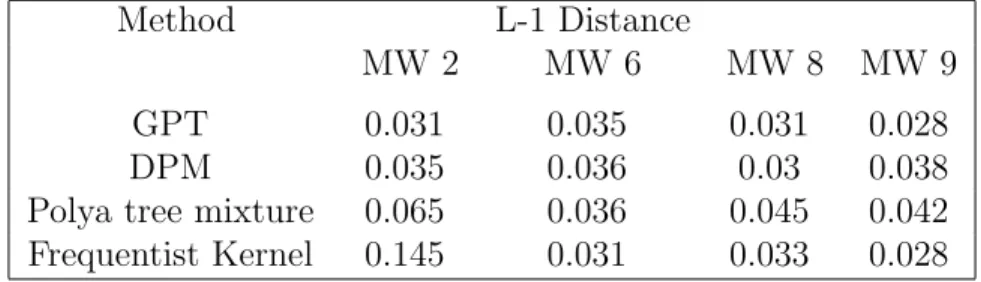
A.1 Marron-Wand Curves: L-1 error . . . 67
A.2 Predictive MSE & L-1 error . . . 67
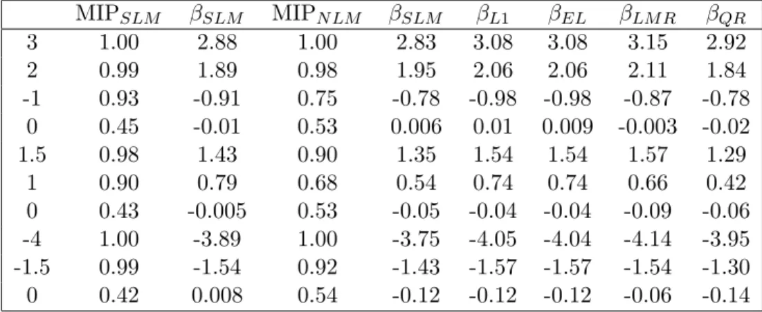
B.1 Estimates and MIPs for fixed effects for Case I when n=100 . . . 78
B.2 Summaries for Case I when n=100 . . . 79
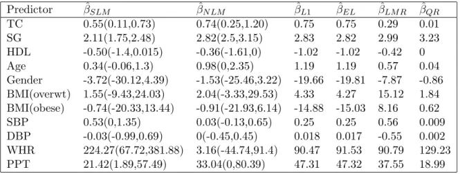
B.3 Fixed effects (times 100) for type-II diabetes example . . . 80
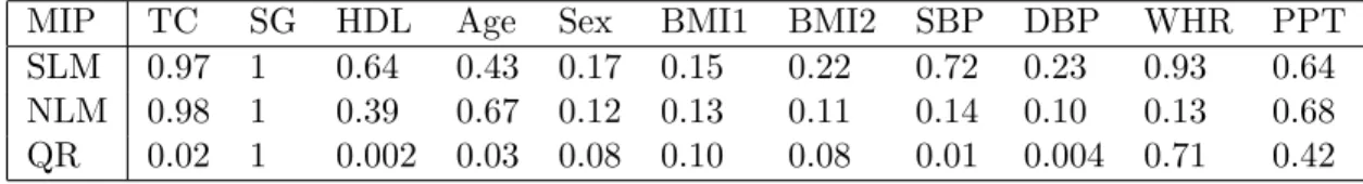
B.4 Marginal Inclusion Probabilities for SLM, NLM and QR . . . 81
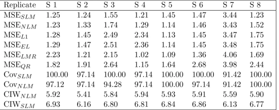
B.5 Prediction (Cov: 95% coverage, CIW: 95% C.I. width) . . . 82
B.6 Auto-correlations across lags for fixed effects . . . 83
C.1 Frequentist Coverage (Fcov) of Credible Regions . . . 89
List of Figures
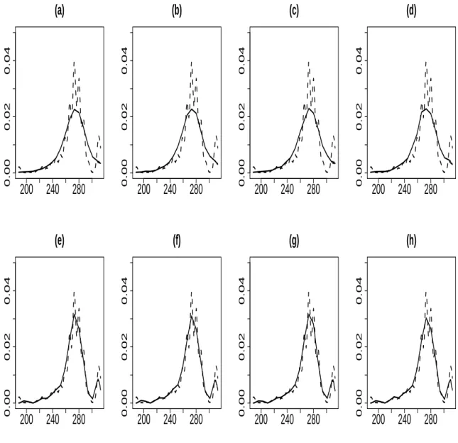
A.1 Prior realizations from the GPT for gestational age
at delivery (solid lines) along with frequentist kernel density estimate (dotted lines). The rows correspond to φ1 = (0.01,0.1);
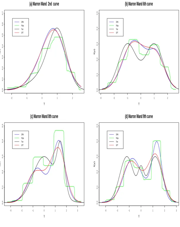
columns correspond to φ2 = (0.1,1,25,100) . . . 68 A.2 Marron-Wand curves - density estimates for GPT, DPM
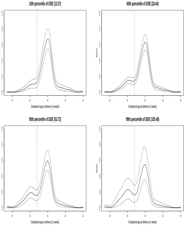
and Polya tree mixtures . . . .69 A.3 GPT conditional density estimates and 90% credible intervals
for 10th, 60th, 90th, 99th DDE quantiles. Vertical dashed line
for cut-off at 37 weeks . . . 70 A.4 DPM conditional density estimates and 90% credible intervals
for 10th, 60th, 90th, 99th DDE quantiles. Vertical dashed line
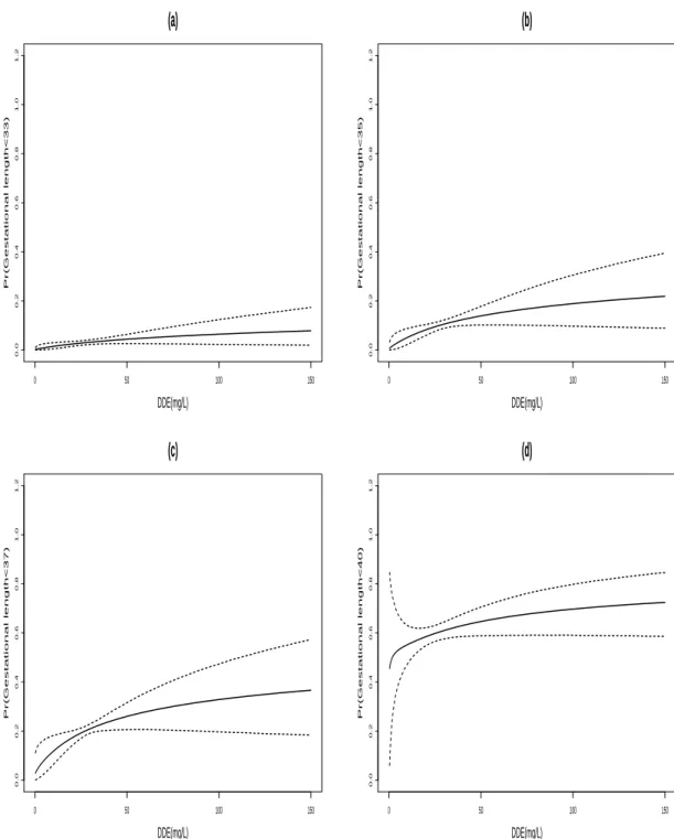
for cut-off at 37 weeks . . . 71 A.5 Estimated probability that gestational age at delivery
is less than T weeks versus DDE dose, for (a) T = 33, (b) T = 35, (c) T = 37, (d) T = 40. Solid lines are posterior means
and dashed lines are pointwise 90% credible intervals . . . 72 B.1 MIP for Case I: Solid lines - SLM, dashed lines - NLM . . . 84 B.2 MIP for Case II: Solid lines - SLM, dashed lines - NLM . . . 85 B.3 Residual plots for Diabetes study for Semi-parametric
Linear Model . . . 86 C.1 Comparison of two dimensional credible regions. Blue Dots:
95% HPD set generated from mixture of bivariate Gaussian and t distribution; Blue line: MVCE credible region
(posterior prob = 0.9507); Red Line: Credible region
Chapter 1
Introduction
1.1
Literature Review and Motivation
1.1.1
Latent Factor Models for Density Estimation
In the first paper of my dissertation, we propose a flexible class of priors for density estimation based on random nonlinear functions of a uniform latent variable with an additive residual. It is well known that nonparametric kernel mixture models are increasingly popular in density estimation, density regression and high dimensional data modeling. Kernel mixture models for density estimation have the form
f(y;G) =
Z
K(y;θ)G(dθ), (1.1)
where G(·) is a mixing distribution and K(·) is a probability kernel. The majority of the nonparametric Bayesian development in this area relies on Dirichlet process (DP) priors (Ferguson, 1973; 1974) for G. A DP on (χ,A) with parameter α is es-sentially a stochastic process where, for any measurable paritition (A1, . . . , Ak) of χ,
the random vector (P(A1), . . . , P(Ak)) follows a Dirichlet distribution with parameters
(α(A1), . . . , α(Ak)). The seminal paper by Ferguson (1973) shows that if P is a DP
distribution of P givenX1, . . . , Xn is also a DP on (χ,A) with parameter (α+
Pn
1 δx).
Ghosal, Ghosh and Ramamoorthi (1999) provided general conditions in terms of L1 metric entropy to ensure strong posterior consistency and verified those conditions for Dirichlet process location mixtures of normal kernels under certain regularity condi-tions. Tokdar (2006) extended their result to the location-scale mixture case while encompassing a significantly larger class of ‘true’ densities. Sethuraman (1994), gave a constructive definition of DP of the form
P =
∞
X
j=1
wjαj, αj ∼N(0, τ−1), wj =νj
Y
l<j
(1−νl), νl ∼Beta(1, m),
which enabled posterior computation involving DP kernel mixtures to become much more manageable. The weights wj are called stick-breaking weights as they can be
obtained by repeatedly breaking a stick of initial length 1 into proportions νh and
1−νh, and continuing the proces with the fraction 1−νh. Pati, Dunson and Tokdar
(2011) has also shown large support and weak/strong posterior consistency for a broad class of generalized stick-breaking priors, which includes the Chung and Dunson (2009) probit stick-breaking prior as a special case. Walker (2007) proposed the slice sampler which greatly improved computational speed. His method relies on augmentation with uniform latent variables as follows
fw,α(y) =
X
j∈Bw(u)
N(y|αj), Bw(u) = {j :wj > u}.
our prior on a prior guess for the density.
These models have been generalized to density regression by defining dependence on the covariates x in various ways. If the covariates have a finite number of levels the Product of Dirichlet processes model introduced by Cifarelli and Regazzini (1978) allows the modelling of dependent distributions. Dependence is introduced through the use of a parametric regression model as the centering distribution of independent Dirichlet processes at each level of the covariates. M¨uller, Elkanli and West (1996) used a DP mixture of multivariate normals to jointly model the density of the response and predictors to induce a prior on f(y|x). Their development boils down to a local linear regression of the form E(y|x, θ)=Pk
j=0sj(x)mj(x), where mj(x) is the mean of the jth component distribution of y given x, which is linear due to the normality of the kernels. The regression weights sj(x) determine that components mj(x) will be more
highly weighted in predicting y when the value of the densityfj(x|θ) is relatively large.
In order to let the parameters of the DP vary over the predictor space X, MacEachern (1999) defined dependent Dirichlet processes (DDP) by assigning stochastic processes on the components in Sethuraman’s (1994) DP representation: Gx =P
∞
i=1pi(x)δθi(x).
This ensures that the parameters of the non-parametric prior are able to adapt across the parameter space, thus giving it more flexibility. De Iorio et al. (2004) proposed a fixed-p DDP in ANOVA models, while Griffin and Steel (2006) introduce dependence in nonparametric distributions by making the weights in the Sethuraman (1994) repre-sentation dependent on the covariates. They modeled each weight as a transformation of i.i.d. random variables and implemented the dependence by inducing an ordering of these random variables at each covariate value such that distributions for similar covariates values will be associated with similar orderings and, thus, be close. At any covariate value, the random distribution would be a so-called stick-breaking prior, and they focused on the special case where they assigned DP for the stick breaking prior.
Dunson, Pillai and Park (2007) instead used predictor-dependent convex combinations of DP components. More specifically, they introduced kernel stick breaking processes of the form
Gx =
∞
X
h=1
U(x;Vh,Γh)
Y
l<h
1−U(x;Vl,Γl)
G∗h U(x;Vh,Γh) =VhK(x,Γh)for all x ∈ X.
HereVh ∼Be(ah, bh),Kh :<p× <p →[0,1] is a bounded kernel function andG∗h is the
base measure located at Γh. ThusGx is a predictor-dependent mixture over an infinite
sequence of basis probability measures. Such a construction can encourage sparsity and borrowing of information acrossX through careful choice of hyper-parameters and kernelsKh.
complex systems involving correlated variables in high-dimensional spaces. FA aims principally to reduce the dimensionality of the data by projecting high-dimensional vectors on to lower-dimensional spaces. However, because of its inherent linearity, the generic FA model is essentially unable to capture data complexity when the input space is nonhomogeneous. A finite Mixture of Factor Analysers (MFA) is a more flexible extension of the basic FA model that overcomes the above limitation by assigning a mixture distribution to the latent factors. The structure of the MFA model offers the potential to model the density of high-dimensional observations adequately while also allowing both clustering and local dimensionality reduction. Chen et al. (2009) and Carvalho et al. (2008) proposed nonparametric Bayes MFA where they allowed an uncertain number of factors by placing DP and Beta process priors respectively on the the number of factors. On the other hand, Dunson (2006) used dynamic mixtures of DPs to allow a latent variable distribution to change nonparametrically across groups. Lee, Lu, and Song (2008) placed a truncated DP on the distribution of the exogenous latent variables within a structural equation model (SEM). In order to ensure identifiability and interpretability in SEM, Yang and Dunson (2010) modelled the exogenous variable using centered Dirichlet processes (CDP) (Yang et al., 2010) in a latent class model and CDP mixtures in a latent trait model. To review, the SEM is specified using two components, (1) the measurement model, which relates the measurement variables to latent variables; and (2) the latent variable or structural model, which describes relationships among the latent variables, typically through a linear structural relations or LISREL model.
The above approaches relying on discrete mixture models, have a number of well known complications motivating alternative methods for modeling unknown densities, such as Polya trees (Mauldin et al, 1992; Lavine, 1992, 1994) and logistic Gaussian processes (LGP) (Lenk 1988, 1991; Tokdar 2007). The Polya tree generates random
probabilities G, such that for any partitioning subset B ( = (1, . . . , m)), G(B) =
Qm
j=1,j=0Y1,...,j−10
Qm
j=1,j=1(1−Y1,...,j−10), where Y0 ∼Be(α0, α1). Polya trees have
appealing properties in terms of denseness, conjugacy and posterior consistency but have disadvantages in terms of favoring overly spiky densities. On the other hand LGP’s are defined as fw(t) = e
w(t)
R
ew(s)ds, where w(·) is assigned a GP prior. The smoothness
properties of the GP transfers on to the LGP, thus rendering it sound theoretical properties and control over the smoothness of the densities through the covariance kernel in the GP. However, posterior computation is a major hurdle. Recently, Jara and Hanson (2010) proposed dependent tail-free processes where they modeled the tail-free probabilities with LGP dependent on covariates. Their approach is shown to approximate the Polya tree marginally at each predictor value. An alternative was suggested by Tokdar, Zhu and Ghosh (2010) relying on LGP for density regression with dimensionality reduction. More specifically, they modeled the conditional density by equivalently modelling quantities such asp(G0(y)|F(z)) using LGP, whereG0 is any cumulative distribution function, F is a d-dimensional function having monotonically increasing components from < to (-1,1) and z belongs to the d-dimensional central subspace of the predictor spaceX.
models. Unlike LGP-based models, the proposed model has conjugacy properties fa-cilitating posterior computation. In addition, the method has appealing theoretical properties in terms of large support and posterior consistency.
Relative to some density estimation priors, the proposed latent factor approach is quite easy to generalize to more challenging settings involving multivariate densities, conditional density estimation, hierarchical modeling and other complexities. Although our primary focus in this article is to introduce the formulation, providing a basic intu-ition for how the model works, basic properties and computation, we also give a flavor of generalizations through a simple conditional density estimation example. In particular, we consider a model that induces a prior on the conditional densityf(y|x) through joint modeling of the response and predictors through separate nonparametric latent factor models containing the same latent variables. This formulation is completely flexible in the marginal densities, while making strong restrictions on the dependence to address the curse of dimensionality in a related manner to a copula model. An attractive fea-ture of our model is that it naturally allows for incorporation of prior information on the marginal densities of response and predictors through the mean function of the GP.
1.1.2
BVS in Semiparametric Linear Models
BVS or Bayesian variable selection is very widely applied, with a rich literature on alternative priors and computational methods. For a recent review of Bayesian variable selection methods, refer to O’Hara and Sillanp¨a¨a (2009). Most of the liter-ature has focused on Gaussian linear regression models, with common methods in-cluding stochastic search variable selection (SSVS) (George and McCulloch, 1993; 1997), reversible jump MCMC (Green, 1995) and adaptive shrinkage (Tibshirani, 1996; Park and Casella, 2008; Yi and Xu, 2008). SSVS puts the prior on effect sizes as
P(βj|Ij) = (1−Ij)N(0, τ2) +IjN(0, gτ2), where Ij is the variable inclusion indicator
and the first density is centered around 0 and has a small variance. The specification of parametersτ, g are data-dependent. Alternatively, SSVS could involve a point mass at 0 instead ofN(0, τ2) in the above formulation. Reversible jump MCMC is a flexible technique for model selection, which lets the Markov chain explore spaces of different dimensions. For variable selection, the positions (indices) of the selected variables are defined as l1, . . . , lNv , and the model is updated by randomly selecting variable j and
then proposing either addition to (Nv := Nv + 1) or deletion from (Nv := Nv − 1)
the model of the corresponding effect. The length of the parameter vector is therefore not fixed but varies during the estimation. The updating is done using a Metropolis-Hastings algorithm, but with the acceptance ratio adjusted for the change in dimension. The degree of sparseness can be controlled by setting the prior for Nv. On the other
the exponential family (Raftery and Richardson 1993; Meyer and Laud 2002).
It is well known that Bayesian variable selection can be sensitive to the prior, and there is an increasingly rich literature showing asymptotic properties providing support for carefully-chosen priors, such as mixtures of g-priors (Zellner and Siow, 1980; Liang et. al., 2008), with such priors also having appealing computational properties. This literature is essentially entirely focused on Gaussian linear regression models, and the emphasis of this article is on developing methods that generalize this work to semiparametric regression models having unknown residual distributions.
To set the stage, first consider the well-studied problem of comparison of linear models of the following type:
M1 :Yn = α1n+Xγ1βγ1 +1, 1 ∼N(0, τ
−1I
n),
M2 :Yn = α1n+Xγ2βγ2 +2, 2 ∼N(0, τ
−1I
n), (1.2)
where Yn is n×1 vector of responses, α is the common intercept, X
γj is a n×pj design
matrix (j=1,2) excluding the column of intercepts, and j’s are Gaussian residuals,
j=1,2. The models may or may not be nested, and the number of candidate predictors is p. Among numerous model selection criteria available for such comparisons, the Bayes factor (Kass and Raftery, 1995) has received substantial attention as the most widely accepted Bayesian measure of the weight of evidence in the data in favor of one model over another. The Bayes factor for comparing M1 versusM2 based on a sample Yn is defined as BFn
12 =
L(Yn|M
1)
L(Yn|M
2), the ratio of marginal likelihoods under M1 and M2.
Assuming one of the models under comparison is true, Bayes factor consistency refers to the phenomenon where BFn12 → ∞P as n → ∞ under M1 and BFn12
P
→ 0 as n → ∞
underM2. A stronger form of consistency is also possible when the convergence happens almost surely. When comparing the true model pairwise to each model in a list, Bayes
factor consistency typically implies that the posterior probability on the true model goes to one.
Although priors most commonly used in practice assume a priori independence in the elements of the coefficient vectors (β1 and β2), priors that have been shown to result in Bayes factor consistency typically incorporate dependence. Examples include the intrinsic prior (Berger and Pericchi, 1996; Moreno, 1997; Moreno, Bertolino and Racugno, 1998) which builds a prior for the alternative model with varying degrees of concentration around the null, and Zellner’s g-prior (Zellner, 1986) specified by
βj ∼ N(0, gτ−1(Xj0Xj)−1), j=1,2. The intrinsic priors have proven to behave very well
for multiple testing problems (Casella and Moreno, 2006). Moreno and Gir´on (2005) showed consistency for the intrinsic Bayes procedure for nested linear models, while Casella (2009) extended consistency for the intrinsic Bayes procedure to non-nested linear models. Zellner’s g-prior allows for a convenient correlation structure and can control for the amount of prior information relative to the sample through only one hyperparameter g. Among others, Fern´andez et al. (2001) investigated Bayes factor consistency under various choices of fixedg, which was allowed to depend on the sample size and/or the number of candidate predictors. In order to resolve difficulties associated with a fixed choice of g, such as Bartlett’s paradox (Bartlett, 1957; Jeffreys 1961) and information paradox (Zellner 1986; Berger and Pericchi 2001), Zellner and Siow (1980) placed an inverse-gamma prior on g, while Liang et. al. (2008) extended the idea of Strawderman (1971) to the regression context by proposing hyper-g and hyper-g/n
priors ong, under which they established Bayes factor consistency. To review, Bartlett’s paradox refers to the fact that in the limiting case wheng → ∞while (n, pγ) are fixed,
the Bayes factor for comparing Mγ to the null model will go to 0. That is, large spread
the information in the data. On the other hand, the information paradox refers to the fact that the Bayes factor in favor of Mγ goes to a constant for a fixed choice ofg as the
coefficient of determination of Mγ goes to 1 (i.e. when there is overwhelming evidence
in favor of Mγ,), keeping (n, pγ) fixed. This is against conventional wisdom, as one
expects the Bayes factor in favor of Mγ to go to ∞ as evidence against the null model
accumulates. Coming back to the afore-mentioned approaches, they entail specifying improper priors on common model parameters and proper priors on model parameters unique to any one model, which results in a prior specification for the more complex model depending upon the simpler model. To avoid such pitfalls, Guo and Speckman (2009) adopted the idea of Marin and Robert (2007) and placed mixtures of g−priors on all the elements of bothβ1 andβ2, which leads to tractable Bayes factors as well as Bayes factor consistency.
There has also been a growing interest in model selection procedures for normal linear models when the number of candidate predictors (p) increase with sample size (n). Such increases occur in a wide variety of applications, such as in nonparamet-ric regression when the number of candidate kernels or basis functions depends on n. Shao (1997) analyzed the consistency of several frequentist and Bayesian approximation criteria for model selection in normal linear models with increasing model dimensions, assuming the true model to be the submodel minimizing the average squared prediction error. Moreno et. al. (2010) examined consistency of Bayes factors and the BIC under intrinsic priors for nested normal linear models, when the dimension of the parameter space increases with the sample size. Jiang (2007) considered Bayesian variable selec-tion in generalized linear models in p > n settings and provided conditions to obtain near optimal rates of convergence in estimating the conditional predictive distribution, but did not consider asymptotic properties in selecting the important predictors.
To our knowledge, this area has entirely focused on parametric models with a
particular focus on normal linear regression. Such a parametric assumption on the residual error is rather stringent and may not hold in practice, thus invalidating the earlier assumption of the true model belonging to the class of models under comparison and potentially leading to inconsistent Bayes factors. Simulations illustrate that when residuals are generated from a bimodal distribution, Bayesian variable selection under a Gaussian linear regression model tends to have poor performance. With this motivation, our focus is on developing Bayes variable selection methods that do not require Gaussian residuals and that can be shown to be consistent.
the cluster structure. They updated the variable selection index using a Metropolis algorithm and obtained inference on the cluster structure via a split-merge Markov chain Monte Carlo technique. Mostofi and Behboodian (2007) model a symmetric and unimodal residual density using a Dirichlet process scale mixtures of uniforms, while conducting Bayesian variable selection by selecting the highest posterior probability model. Chung and Dunson (2009) modeled the conditional response density given predictors using a flexible probit stick-breaking mixture of Gaussian linear models, allowing variable selection via a Bayesian stochastic search method. More specifically, they introduced the probit stick-breaking process (PSBP) as a prior for an uncountable collection of predictor-dependent random probability measures and proposed a PSBP mixture (PSBPM) of normal regressions for modeling the conditional distributions. They incorporated a global variable selection structure so as to discard unimportant predictors, while allowing estimation of posterior inclusion probabilities. Further, they did local variable selection while relying on the conditional distribution estimates at different predictor points.
These articles focused on defining methodology and computational algorithms, but without study of theoretical properties, such as consistency. In fact, to our knowl-edge, there has been no previous work on consistent Bayesian variable selection in semi-parametric models, though there is recent work on consistent non-semi-parametric Bayesian model selection (Ghosal, Lember and van der Vaart, 2008 among others). Ghosal, Lember and van der Vaart (2008) considered nonparametric Bayesian estimation of a probability density based on a random sample of size n from this density using a hierarchical prior. They presented a general theorem on the rate of contraction of the resulting posterior distribution asn → ∞which gives conditions under which the rate of contraction is the one attached to the model that best approximates the true density of the observations. This shows that, for instance, the posterior distribution can adapt
to the smoothness of the underlying density. They also studied the posterior distri-bution of the model index, and found that under the same conditions the posterior distribution gives negligible weight to models that are bigger than the optimal one, and thus selects the optimal model or smaller models that also approximate the true density well. However, it is not straightforward to apply such theory directly to the problem of variable selection in semiparametric linear models.
With this motivation, we define a practical, useful and general methodology for Bayesian variable selection in semiparametric linear models, while providing basic the-oretical support by showing Bayes factor and variable selection consistency. We accom-plish this by generalizing the methods and asymptotic theory for mixtures of g-priors to linear regression models with unknown residuals characterized via Dirichlet process (DP) location mixture of Gaussians. We propose a new class of mixtures of semi-parametric g-priors under a family of proper priors for g, which results in consistent Bayesian variable selection even when there are many more candidate predictors (p) than samples (n) as long as the prior assigns probability zero to models having greater than or equal to n predictors. Additionally, posterior computation for the proposed method is straightforward via a SSVS algorithm.
1.1.3
Bayesian credible regions for vectors and functions
for estimating HPD regions for vectors or functions. Current state-of-the-art methods for Bayesian estimation of credible regions focus on using either large sample elliptical regions that can be justified by asymptotic normality of the posterior or rectangular regions that inflate the size of scalar regions for each parameter using multiplicity adjustments. Given the routine use of credible sets in practice, there is a clear need for improved methods for efficiently estimating minimum volume credible sets for vectors and functions based on MCMC output.
To adjust for conservatism while maintaining a rectangular region, Crainiceanu et al. (2007) assumed approximate posterior normality and proposed inflated hyper-rectangular regions as
ˆ
θj −c1−α
q
d
var(θj),θˆj+c1−α
q
d
var(θj);j = 1, . . . , p
,
where ˆθ= (ˆθ1, . . . ,θˆp)0 is the posterior mean of the parameter of interestθ= (θ1, . . . , θp)0,
and c1−α is the 1−α percentile of maxj=1,...,p
θs
j−θˆj
√ d
var(θj)
with θ
s corresponding to the
sth MCMC draw from the posterior.
Unfortunately, restricting consideration to rectangular regions ignores the true topology of the joint posterior and can lead to 100(1−α)% credible regions that can have dramatically larger volume than necessary. As an alternative for estimating convex credible regions based on MCMC samples, we initially considered convex hull peeling in which one starts with the convex hull of the MCMC samples and peels off outer layers by discarding outer points until obtaining a region containing 100(1−α)% of the samples. Although such an approach is promising, even fast algorithms for calculating the convex hull of a set of points have substantial computational burden. For example, the worst case complexity of the quick-hull algorithm (Barber et. al, 1996) is O(nfr/r)
forp >3, where ris the number of processed points and fr is the maximum number of
faces forrvertices. The number of processed points is much larger thanp, implying that
fr =O(rbp/2c/bp/2c) (Klee, 1966) increases rapidly aspincreases, so that computation
becomes unmanageable quickly. Hence, we do not consider such an approach further. In developing an alternative, we use the equivalence between HPD regions, mini-mum volume (MV) sets and density level sets of the posterior to ascertain the subset of MCMC samples falling within the HPD region. MV sets (Polonik, 1995, 1997) summarize regions with a pre-assigned probability content where the mass is most con-centrated, and are closely related to density level sets (Tsybakov, 1997; Ben-David and Lindenbaum, 1997; Cuevas and Rodriguez-Casal, 2003; Steinwart et al., 2005). The main difference is that the latter requires the specification of a density level of interest instead of the probability mass to be enclosed. The equivalence between MV sets and density level sets was established by Nunez-Garcia et al. (2003) under some reasonable conditions.
Assuming that the posterior g(θ|Yn) ∝ h(θ, Yn) = π(θ)L(Yn|θ) (L(·) being the
likelihood) is known up to a normalizing constant, we can exploit the aforementioned equivalence to assert that any posterior MCMC sample θj, j=1,. . . ,J, satisfying
h(θj, Yn)> λ, P{θ:h(θ, Yn)> λ|Yn}= 1−α, (1.3)
will belong to the 100(1−α)% HPD credible region. An estimate for λ can be ob-tained from the MCMC samples as ˆλ such that #{θ
j:h(θj,Yn)≥λˆ}
J ≥ 1 − α. To
al-low for additional parameters ψ in the model without requiring a known analytic form for the marginal h(θ, Yn) = R
L(Yn|θ, ψ)π(θ|ψ)π(ψ)dψ, we can rely on an
ap-proximation, with a simple choice corresponding to the Monte Carlo approximation ˆ
h(θ, Yn) = 1/HPH h=1L(Y
n|θ, ψh)π(θ|ψh), where ψhs (h = 1, . . . , H) are realizations
from the prior π(ψ). Such an approximation is not possible under improper priors for
We propose a method for constructing elliptical credible regions which enclose the 100(1−α)% HPD set defined as the collection of posterior MCMC samples satis-fying (1.3), with the estimated density level ˆλ. In the presence of nuisance parameters, we replace h(θ, Yn) with ˆh(θ, Yn). In cases when such an approximation is poor, the
HPD set may contain samples outside of the 100(1−α)% HPD region, thereby po-tentially yielding slightly inflated finite dimensional credible regions. Elliptical regions provide a convenient approximation, with the exact credible region having an ellipti-cal form under multivariate normality of the posterior. Bernstein von Mises theorems guarantee asymptotic normality for sufficiently regular parametric models, with similar results arising in certain semi- or nonparametric models (Castillo, 2012; Rivoirard and Rousseau, 2009). Our approach utilizes minimum volume covering ellipsoids (MVCE) (Rousseeuw 1985), which have been implemented in a variety of application areas (Knorr et al., 2001; Kumar and Orlin, 2008). Typically approximate algorithms are used (Khachiyan, 1996; Kumar and Yildirim, 2005; Sun and Freund, 2004), as exact computation is often not feasible.
Another major focus of our paper is constructing credible regions for functions. Although there is a rich literature on Bayesian semi- and nonparametric methods, with recent theoretical results on properties of credible regions for functions (Knapik, van der Vaart and van Zanten, 2011), there is a surprising lack of methods for calculating such regions in practice. Most commonly one reports pointwise intervals for the function at different locations or for functionals of interest. However, this clearly provides an inadequate characterization of uncertainty in the function as a whole. Simultaneous credible regions have useful applications in hypothesis testing for random functions. For example, we might conclude that a curve is well approximated by a parametric function if the parametric curve falls entirely within the estimated credible region. In addition, there is often interest in assessing whether the region includes a flat line
or surface corresponding to a null hypothesis under consideration. In nonparametric regression, such a null hypothesis may correspond to there being no effect of a predictor or predictors of interest. In other settings, the null corresponds to there being no difference in group-specific surfaces.
Chapter 2
Latent Factor Models for Density
Estimation
2.1
Model Specification
Initially suppose yi ∈ < are iid draws from an unknown density f ∈ F, where F
is the set of densities on < with respect to Lesbesgue measure. We propose to induce a priorf ∼Π through
yi = µ(xi) +i, i ∼Γσ,
µ∼Π∗, σ ∼ ν, xi ∼Uniform(0,1), (2.1)
where µ ∈ Θ is an unknown [0,1] → < function, xi is a uniformly distributed latent
variable, and the error distribution Γσ is centered at 0 and has scale parameter σ.
Hence, in the special case in which µ(x) = µ, so that the regression function is a constant, and Γσ is normal, we have f(y;µ, σ2) = N(y;µ, σ2) so we obtain a normal
density. The density of y conditionally on the unknown regression functionµ and σ is obtained on marginalizing out the latent variable as
f(y;µ, σ) =fµ,σ(y) =
Z 1
0
To complete the specification, we letµ∼Π∗, σ∼ν and obtain the marginal density
f(y) =
Z ∞
0
Z
Θ
Z 1
0
Γσ(y−µ(x))dxΠ∗(dµ)ν(dσ). (2.3)
Hence, a prior f ∼ Π is induced through assigning independent priors to µ and σ in expression (2.2). When the prior on µis a Gaussian process and the error distribution isN(0, σ2) (denoted as Γ
σ =φσ), we refer tofµ,σ as a Gaussian process transfer (GPT)
model and the induced prior f ∼Π as a GPT prior.
The GPT prior does not have the kernel mixture form (1.1). There will be no clustering of subjects or label switching issues. Instead, the prior f ∼ Π is induced through adding a Gaussian residual to a Gaussian process regression model in a uniform latent variable. This is a simple structure aiding computation and interpretability. One can control the smoothness of the density through the covariance in the GP prior for the regression function µ and the size of the scale parameter σ. In limiting cases, one can obtain realizations ofµconcentrated close to a flat line, leading to a normal density as a special case. In addition, by makingσsmall and choosing the GP covariance to generate a very bumpyµ, one can obtain arbitrarily bumpy densities. In practice, by choosing hyperpriors for key covariance parameters, we obtain a data adaptive approach that often outperforms discrete kernel mixtures. The performance of discrete kernel mixtures relies on the ability to accurately approximate the density with few components, and DP mixtures tend to heavily favor a small number of dominate kernels. This tendency can sometimes lead to relatively poor estimation, as illustrated in section 2.7.
2.2
Prior Specification
many parameters. Most of the Bayesian nonparametrics literature relies on default pri-ors, which do not reflect available prior knowledge in a particular application area, but are chosen to lead to good performance in terms of posterior behavior in a wide variety of applications. However, as in parametric models, well chosen informative priors that utilize information, such as historical data on the variables under study, can substan-tially improve the performance in small to moderate samples. In DP mixtures, such prior information is typically incorporated through choice of hyperparameters in the base measure, while maintaining conjugacy for ease in computation. For example, in Gaussian kernel mixtures, a normal-inverse gamma base measure would be chosen hav-ing parameters representhav-ing prior knowledge. This is appropriate when prior knowledge implies that the density follows a t distribution, but when one has prior information that the density follows a more complex form (as in our premature delivery application) then elicitation is substantially more difficult. Obtaining a base measure that leads to a particular elicited density is a deconvolution problem, which can be difficult to solve for non-atomic base measures. In addition, posterior computation under the resulting complex and non-conjugate base measure may be challenging. An advantage of the GPT is that the prior for the density can be centered on an arbitrary choice easily through the prior mean in the GP prior forµ.
To elaborate, Theorem 3 (section 2.3) ensures that µ ≈ µ˜ = ˜F−1 implies that
fµ,σ ≈ fµ,σ˜ = ˜f, with ˜f = dydF˜ and σ ≈ 0. In terms of application, this translates to incorporating a prior guess ˜f for the density through the corresponding mean function ˜
µ = ˜F−1 of the GP, and letting the prior for σ to have mode near 0. Such a mean function can be constructed by obtaining frequentist kernel estimates of the concerned density using some external data, and then converting it into an inverse cdf on a grid of points in [0,1] (using a linear approximation). Thus, the characteristics of the entire density is captured through ˜F−1 as the mean function of the GP, and we let the data
influence the deviation of the posterior from the prior guess.
These ideas are demonstrated in Figure A.1, where we use some earlier data on gestational age at delivery to construct prior densities. We choose a Ga(25,1) prior for the residual precision, and different sets of hyper-parameters for the covariance kernel of the GP. The frequentist kernel estimates were obtained by the bandwidth selection method of Sheather and Jones (1991), using a Gaussian kernel (‘kernel’ function in R). It is evident that the smoothness as well as the degree of deviation of the prior from the frequentist estimate can be controlled through the hyper-parameters in the covariance kernel of the GP.
2.3
Theoretical Properties
To further justify the proposed prior, we show large support and posterior con-sistency properties. Large support is an important property in that it ensures that our prior can generate densities that are arbitrarily close to any true densityf0 in a large class, a defining property for a nonparametric Bayesian procedure and a necessary con-dition to allow the posterior to concentrate in small neighborhoods of the truth. Instead of focusing narrowly on GPT priors, we provide broad theoretical results for priors in the general class of expression (3.1).
Before proceeding, it is necessary to define some notation and concepts. We denote the Kullback-Leibler (KL) divergence of fµ,σ from f0 as KL(fµ,σ, f0) and an
−sized KL neighborhood around f0 asKL(f0) ={fµ,σ :KL(fµ,σ, f0)< }. The sup-norm distance is denoted by ||.||∞. We note that, to generate yi ∼ f0, one can draw
xi ∼Uniform(0,1) and letyi =F0−1(xi),F0−1 being the inverse cdf on<(assumingF
−1 0
the cdf of fµ0,σ. More precisely,
(A1): The true (data generating) density can be represented as the limiting case
f0(y) = lim
σ→0
Z 1
0
Γσ(y−µ0(x))dx∈(0,∞), (2.4) whereµ0 =F0−1, for all y∈ < and assuming Γσ is chosen so that such the limit exists.
Since the limiting distribution of model (3.1) can be used to generate samples from any arbitrary distribution,(A1) includes the class of all strictly positive and finite densities for which convergence in distribution implies convergence of the corresponding density functions. Further in the proofs, we will also repeatedly use the fact that for µ close toµ0 and σ ∈ <+, logfµ,σf0 <∞ for f0 defined in (A1) and Γσ = Gaussian or Laplace.
For notational convenience, we will often useµandµ(x) interchangeably in the sequel. Theorem 1 Let Γσ be normal or Laplace having scale parameter σ withf0 being the
corresponding density in F defined as in (A1). If Π∗⊗ν
(µ, σ) :||µ−µ0||∞< η1, σ∈
(0, η2)
>0for arbitrarily small(η1, η2)>0, then Π(KL(f0))>0for all(η1, η2)>0. Theorem 1 allows us to verify that the induced prior on the density f assigns positive probability to KL neighborhoods of any strictly positive and finite true density
f0. From Schwartz (1965), if the true densityf0 is in the KL support of the prior for
f, the posterior distribution for f will concentrate asymptotically in arbitrarily small weak neighborhoods of f0. Theorem 1 requires the prior µ ∼ Π∗ to place positive probability in sup-norm neighborhoods of the inverse cdfF0−1. Although one can verify this condition for certain choices of Π∗, such as appropriately chosen Gaussian process priors, it is nonetheless somewhat stringent. We show in Theorem 2 that this condition can be relaxed to only require that the prior µ∼Π∗ assigns positive probability to L-1 neighborhoods of any elementµ0 of Θ. It is well known that positive sup-norm support automatically guarantees positive L-1 support but the converse is not true. Let us
denote an1-sized L-1 neighborhood aroundµ0 asN1(µ0) =
fµ,σ :
R
|fµ,σ−f0|< 1 . Theorem 2 Let Γσ = φσ and f0 be the corresponding density in F defined in (A1).
If Π∗ ⊗ν{(µ, σ) :µ∈Nη1(µ0), σ∈(0, η2)} > 0 for arbitrarily small η1, η2 > 0, then
Π(KL(f0))>0 for all (η1, η2)>0.
As the prior f ∼Π is specified indirectly through priors µ∼Π∗ and σ ∼ν, it is desirable for elicitation purposes to verify that, for sufficiently small σ, µ ≈ µ˜ = ˜F−1 implies that fµ,σ ≈ fµ,σ˜ = ˜f, where ˜f = dydF˜. Theorem 3 provides such a verification assuming Gaussian errors. This implies one can potentially center the prior for the densityf on an initial parametric guess ˜f by centering µ∼Π∗ on the inverse cdf ˜F−1
while choosing the prior forσ to have mode near zero. The data will then inform about the degree to whichµ deviates from ˜F−1 and σ deviates from 0.
Theorem 3 Supposef˜= limσ→0
R1
0 φσ(y−µ˜(x))dx, where µ˜= ˜F
−1, the inverse cdf
corresponding to f˜. Then for µ∈N1(˜µ) andσ ∈(2,
∗
2), we have fµ,σ ∈N1
2
˜
f for
arbitrarily small 1, 2, ∗2 such that 0< 1 < 2 < ∗2.
(A2): Suppose µ∼ GP(m, c) such that the mean function m(·) is continuously differ-entiable with supxm(x)<∞, and the covariance function c(·,·) has continuous fourth
derivatives.
Theorem 4 Suppose (A2) holds and define f0 as in (A1) where Γσ = φσ. Further
letν(σ∈(0, Ln))< d1exp(−d2n)withd1, d2 >0for large n andlimn→∞Ln= 0. Then,
f0 is in the KL support of Π implies that the posterior is strongly consistent at f0.
The above assumptions can be verified for many popular GP covariance functions, both stationary and nonstationary. Some such examples can be found in Choi et. al. (2004). The proof of the above Theorem relies on Theorem 2 of Ghosal, Ghosh and Ramamoorthi (1999), which is listed as Theorem 5in Appendix A.
2.4
Single Factor Density Regression
As a simple and parsimonious single factor model that generalizes the model of Section 2.1 to include predictorszi = (zi1, . . . , zip)0 of a responseyi, we let
yi = µY(xi) +i, i ∼N(0, σY2),
zik = µZk(xi) +∗ik,
∗
ik ∼N(0, σ
2
Zk), k = 1,2, . . . , p,
xi ∼ Uniform(0,1),
µY ∼ ΠY, µZk ∼ΠZk, k = 1,2, . . . , p,
σY ∼ ν, σZk ∼ν, (2.5)
where µY, µZk ∈ Θ are unknown [0,1] → < functions, ’s are independent errors and
xi is the latent variable. For simplicity, we assume the same prior ν on the precision
of the measurement errors in each component model, though this assumption is trivial to relax. Expression (2.5) is a multivariate generalization of the univariate density
estimation model (3.1). Marginally each of the variables is assigned exactly the prior in (3.1) and to allow dependence we incorporate the same latent factor xi in each of
the models.
Our goal in defining a joint model is to induce a flexible but parsimonious model for the conditional density of yi given the predictors zi. In estimating conditional
densities for multiple predictors, one encounters a daunting dimensionality problem in that one is attempting to estimate a density nonparametrically while allowing arbitrary changes in this density across a multivariate predictor space. Clearly, aspincreases even for large samples there will be many regions of the predictor space that have sparse observations. As a compromise between flexibility and parsimony in addressing the curse of dimensionality, we propose to use a single factor model in which the marginals for each variable are fully flexible but restrictions come in through assuming dependence on a single xi. Extensions to the multiple factor case are straightforward.
2.5
Posterior Computation
For simplicity, we focus on the single predictor density regression case when out-lining an MCMC algorithm for posterior computation. Let Yn×1 and ZN×1 denote the vector of observations and covariates, respectively. We are interested in pre-diction of yn+1, . . . , yN based on zn+1, . . . , zN. Let µnY (n× 1) and µNZ (N ×1)
de-note the (unobserved) realizations of the GP µY and µZ at the latent variable values x = (x1, . . . , xn, xn+1, . . . , xN)0. From the GP prior, we have µnY ∼ Nn(mnY,K
n Y) and
µN
Z ∼ NN(mNZ,K N
Z). Let N(A|B) denote the conditional normal distribution. The
covariance kernels are squared exponential with KY(x, x0) = φ1
Y exp
−CY(x−x0)2
and KZ(x, x0) = φ1Z exp
− CZ(x − x0)2
. We specify conjugate gamma priors:
σ−Y2 ∼ Ga(aσ, bσ), σZ−2 ∼ Ga(aaσ, bbσ), φY ∼ Ga(aφ, bφ) and φZ ∼ Ga(aaφ, bbφ). For
evenly distributed grid pointsg1∗, g2∗, . . . , g∗G∈(0,1). LetµnY(−i) include all elements of
µnY except µY(xi), and similarly for µNZ(−i). The Gibbs sampling algorithm alternates
between the following steps.
Step1: Update σ2
Y and σ2Z using π(σ
−2
Y |−)∼Ga(aσ+n/2, bσ+
1 2
Pn
i=1(yi−µY(xi))2) and
π(σZ−2|−)∼Ga(aaσ+N/2, bbσ+12PNi=1(zi−µZ(xi))2) respectively.
Step2: To sample the latent variables, choose xi =gk∗ with probability pik, where
pik =P[xi =gk∗|−] =
pY
ikpZikN(µY(xi =g∗k)|µnY(−i))N(µZ(xi =gk∗)|µNZ(−i))
PG
l=1p
Y ilp
Z
ilN(µY(xi =g
∗
l)|µ n
Y(−i))N(µZ(xi =gl∗)|µNZ(−i))
, if i≤ n
= p
Z
ikN(µZ(xi =g∗k)|µNZ(−i))
PG
l=1p
Z
ilN(µZ(xi =g
∗
l)|µ N Z(−i))
, if n< i≤ N,
wherepY
ik =N(yi;µY(xi =g∗k), σY2),pZik =N(zi;µZ(xi =gk∗), σZ2) and k=1,2, . . . , G.
Step3: Updateµn
Y andµNZ using π(µnY|−) =Nn
(D−Y1+(KYn)−1)−1(DY−1Y+(KnY)−1mnY),(D−Y1+
(KnY)−1)−1
andπ(µNZ|−) =NN
(D−Z1+(KNZ)−1)−1(D−Z1Z+(KZN)−1mNZ),(DZ−1+(KNZ)−1)−1
,
whereDY=σ2YIn and DZ=σZ2IN.
Step4: Updateµ∗G Y =
µY(g∗
1), . . . , µY(g
∗
G) andµ
∗G Z =
µZ(g∗
1), . . . , µZ(g
∗
G) using the
conditional normal distributions N(µ∗G
Y |µnY) and N(µ
∗G Z |µNZ).
Step5: UpdateφY andφZusingπ(φY|−)∼Ga(aφ+n2, bφ+12(µnY−mnY)
0(Kn Y)
−1(µn Y−mnY)
) and π(φZ|−)∼Ga(aaφ+N2, bbφ+12(µNZ −mNZ)
0(KN Z)
−1(µN
Z −mNZ) ) respectively.
Step6: Update CY and CZ using Metropolis random walk for log(CY) and log(CZ).
For prediction ofykbased onzk, k =n+ 1, . . . , N, we useπ(yk|−) =N(yk;µY(xk), σ2Y),
while the conditional density estimate is calculated as ˆf(y|z) =
1
G
PG
k=1φσY(y−µY(gk∗))φσZ(z−µ
Z(g∗
k))
1
G
PG
k=1φσZ(z−µZ(g
∗
k))
.
2.6
Simulation Study
To assess the performance of the GPT approach in density estimation as well as density regression, we conducted several simulation studies. We chose the mean
function for the GP as m(x)=2sin(x)+cos(x) and utilized the squared exponential co-variance kernel. For computational purposes, we worked with the standardized data and then transformed it back in the final step. The hyperparameters for the gamma priors were chosen to be one throughout. Although we used 75 grid points for the griddy Gibbs approach, the number of points could be as low as 60. The number of iterations used was 10000 with a burn in of 1000. The convergence for the main quantities such asµ was rapid with good mixing. All results are reported over 5 replicates.
2.6.1
Univariate Density Estimation
To see how well the GPT does in practice for density estimation, we looked at a variety of scenarios, where the truth was generated from the densities considered in Marron and Wand (1992), which are essentially finite mixtures of Gaussians. We present the results from four of those cases which we thought to be interesting deviations from normality and could be potentially encountered in applications. These are the 2nd, 6th, 8th and 9th Marron-Wand densities. The sample size used was 100. For comparison, we looked at DP mixture of Gaussians (Escobar and West, 1995), mixtures of Polya trees (Hanson, 2006) and frequentist kernel estimates using a Gaussian kernel (and the bandwidth selection method of Sheather and Jones, 1991). More specifically, for both DP mixtures and mixtures of Polya trees, we used the DP package in R and the standard hyperparameter values therein. We used algorithm 8 of Neal (2000) with m=1 for DP mixtures of Gaussians. For frequentist kernel, we used the function “density” in R with Gaussian kernel. Overall, we found that varying the hyperparameter values within a reasonable range does not significantly alter the density estimation results for a sample size of 100, for any of the competitors. Table A.1 presents the L-1 distance between true and estimated densities while Figure A.2 depicts the density plots.
of Gaussians, the GPT tends to do better or at least as well as the DP mixture of Gaussians. Mixtures of Polya trees have somewhat worse performance and result in overly spiky looking estimates.
2.6.2
Single Factor Density Regression
For density regression, we generated a univariate response by allowing the condi-tional mean as well as the residual error distribution to vary with the covariate. We compared the out of sample predictive performance of GPT with other competitors such as DP mixture of bivariate normals (M¨uller, Erkanli and West, 1996), Bayesian additive regression trees (BART) (Chipman, George and McCulloch, 2010), GP mean regression (O’Hagan and Kingman, 1978) and treed GP (Gramacy and Lee, 2008), based on standard packages in R. We used the DP package for DP mixtures of Gaus-sians and the Bayestree package for the other three methods, and the hyperparameter values therein. The density regression results did not change significantly on varying the hyperparameter values within a reasonable range, for all the competitors. We used the following scheme for simulations:
Z ∼FZ, yi = λexp
− e
zi
1 +ezi
+ e
zi
1 +ezii, i ∼N(0, σ
2 ),
whereFZis the distribution of the predictors which was chosen to be a trimodal density
(9th Marron-Wand curve). We chose λ = 3 and split the total sample size of 100 into training set of 50 and test set of 50. The above data generating model allows the shape of the conditional density to change with predictors, hence making prediction non-trivial. Table A.2 shows the performance of the GPT along with a few competitors. We computed the mean square error (MSE), 95% coverage for the mean (COV), as well as the L-1 distance between true and estimated densities at 25th, 50th and 75th
percentiles of the predictor distribution.
The results in table A.2 are consistent with our experience in simulations- when the predictor distribution is multimodal and the shape of the conditional density is allowed to change with predictors, then the GPT tends to do as well or better than DP mixture of Gaussians. For the above study, the average number of components in the conditional distribution obtained from DP mixtures was around 15 which is quite high for a sample size of 50. As illustrated in table 2, BART, treed GP and the GP mean regression methods are primarily mean regression methods and so cannot possibly do well in terms of characterizing the entire conditional of response given predictors. They might perhaps estimate the mean surface reasonably well, but eventually fail in capturing multimodality or tail behavior, the latter often being an important focus of inferences.
2.7
Epidemiological Application
2.7.1
Study Background
the GAD density with increasing DDE.
2.7.2
Analysis and Results
We used the GPT to analyze the dose response relationship in a subset of 182 women of advanced maternal age (≥ 35 yrs) in the above dataset. We examined the conditional distribution of GAD at 10th, 60th, 90th and 99th percentile of DDE. Further, we looked at the dose response relationship between preterm birth and DDE, by examining the left tail of GAD over varying doses of DDE. We used normalized data for analysis and converted it back in the final step. Using the prior specification approach of section 2.2, we were able to incorporate prior information on the marginal density of GAD (using an external data) through the mean function of the GP. Note that prior on σ−2 for GAD was chosen as Ga(25,1). Given the limited sample size and the complexity of the data we are trying to model, we adjusted other hyperparameter settings to reflect our prior belief about the data. The starting value for the length-scale parameter in the covariance kernel in the Metropolis random walk was chosen to be 25, so as to have smooth Gaussian process prior. Instead of working with DDE, we used log(DDE) which resembled a Gaussian distribution, with a 0 mean function for the predictor component and Ga(1,1) prior for the corresponding residual precision.
Figure A.3 shows the conditional distribution curves for GPT along with 90% credible intervals. Although we focused on a small subsample of 182 women of ad-vanced maternal age, the GPT results for the conditional density are remarkably sim-ilar to the ones reported in Dunson et al. (2008), which suggests that there is no systematic difference for women of advanced maternal age. The conditional densities show an increasing bump in the left tail with increasing DDE, suggesting increased risk of preterm birth at higher doses. This is further supported by dose-response curves
for P(GAD<T) in Figure A.5, with different choices for cut-off T. Although the dose-response curve is mostly flat for T=33 weeks, the relationship becomes more significant as cut-off increases, with the dose-response tapering off at T=40 weeks. This suggests that increased risk of preterm birth at higher DDE dosage is attributable to premature deliveries between 33 and 37 weeks. Trace plots of f(y|z) for different DDE percentiles (not shown) exhibit excellent rates of convergence and mixing. For comparison, Figure A.4 shows the density estimates from the DP mixture of Gaussians which has a ten-dency to overly favor multimodal densities, which is as expected given our simulation study results. These results were obtained using DP package in R (and the data driven hyperparameter values therein), which utilizes algorithm 8 of Neal (2000) with m=1.
2.8
Discussion
Chapter 3
Bayes Variable Selection in
Semiparametric Linear Models
Having proposed an elegant solution based on non-mixture alternatives to the important problem of Bayesian density estimation and density regression, we now turn our attention to another fundamental problem in statistics, namely variable selection. Variable selection involves selecting an important and potentially parsimonious subset of predictors which significantly affects the outcome. As stated in the introduction, majority of the literature has focused on linear regression models involving Gaussian residuals. Our objective is to propose a consistent Bayes variable selection method in linear regression models having unknown residuals, which is expected to perform well in a wide variety of situations due to greater flexibility of the proposed model.
3.1
Model Formulation
process (DP) location mixture of Gaussians. In particular, let
yi = x0γ,iβγ+i, i ∼f, i= 1, . . . , n,
f(·) =
Z
N(·;α, τ−1)dP(α), P ∼DP(mP0), P0 =N(0, τ−1), (3.1)
wherexγ,i is theith row of Xγ and does not include an intercept as we do not restrict
f to have zero mean, and f is a density with respect to Lebesgue measure on <. We address uncertainty in subset selection by placing a prior on γ, while the prior on βγ
characterizes prior knowledge of the size of the coefficients for the selected predictors. The DP mixture prior on the density f induces clustering of the n subjects into
k groups/subclusters, wherek is random and each group has a distinct intercept in the linear regression model. LetAdenote ann×k allocation matrix, withAij = 1 if theith
subject is allocated to thejth cluster and 0 otherwise. Thejth column ofA then sums to nj, the number of subjects allocated to subcluster j, with
Pk
j=1nj = n. Following
Kyung, Gill and Casella (2009), conditionally on the allocation matrix A, (3.1) can be represented as a linear model with random intercepts
Yn =Aη+Xγβγ+, η∼N(0, τ−1Ik), ∼N(0, τ−1In), (3.2)
where A is random with a certain prior probability given by the coefficients in the summation of the likelihood expression (3.7).
as follows:
π(βγ) = N(0, gτ−1(Xγ0Σ
−1
A Xγ)−1), ΣA =I+AA0, g ∼π(g). (3.3)
Prior (3.3) inherits the advantages of the traditional mixtures of g-priors including computational efficiency in computing marginal likelihoods (conditional onA) and ro-bustness to mis-specification of g. In addition, the prior can be interpreted as having arisen from the analysis of a conceptual sample generated using a scaled design matrix Σ−A1/2Xγ, reflecting the clustering phenomenon due to the DP kernel mixture prior.
Moreover, the proposed prior leads to Bayes factor and variable selection consistency in semi-parametric linear models (3.1), as highlighted in the sequel.
Note that since (Xγ0Σ−A1Xγ)−1 ≥ (Xγ0Xγ)−1, the prior variance of Y conditional
on (g, τ) is higher for the semi-parametric g−prior as compared to the traditional
g−prior for any allocation matrix A. To assess the influence of A on the prior for
βγ, we did simulations which revealed that for fixed (n, p), var(βγl) increases but the
cov(βγl, βγl0) decreases as the number of underlying subclusters in the data increase
(l0, l = 1, . . . , p, l0 6=l). This suggests that as the number of groups in A increase, the components of βγ are likely to be more dispersed with decreasing association between
each other.
3.2
Bayes Factor in Semiparametric Linear Models
Throughout the rest of the paper, we will assume that the data Yn=(Y
1, . . . , Yn)0
are generated from the true model MT :Yn =Xγ1βγ1 +, with i i.i.d. from the true
residual density f0, which is a density on < with respect to Lesbesgue measure. For modeling purposes, we put a DP location mixture of Gaussians prior on the unknown
f0. For pairwise comparison, we evaluate the evidence in favor ofM1 compared toM2
using the Bayes factor, where
M1 : Yn=Xγ1βγ1 +1, 1i ∼f
M2 : Yn=Xγ2βγ2 +2, 2i ∼f
f(·) =
Z
N(·;α, τ−1)dP(α), P ∼DP(mP0), P0 =N(0, τ−1)
βγj ∼ π(βγj), j = 1,2, π(τ
−1)∝1/τ−1, g ∼π(g), (3.4)
whereγj ∈Γ indexes models of dimensionpj andπ(βγj) is defined in (3.3),j = 1,2.Our
prior specification philosophy is similar to the one adopted by Guo and Speckman (2009) for normal linear models, in that we assign proper priors on all elements of bothβγ1, βγ2
conditional on (g, τ−1), and an improper prior onτ−1 for a more objective assessment. However unlike Guo and Speckman (2009), our focus is on Bayesian variable selection in semi-parametric linear models.
Note that the conditional likelihood of the response after marginalizing out η in (3.2) is L(Yn|A, β
γ, τ−1) = N(Xγβγ, τ−1ΣA) (Kyung et. al., 2009). Thus conditional
onA and under the DPM of Gaussians prior on f,Mj in (3.4) reduces to the normal
linear model:
Σ−A1/2Yn=ZA= ˜XA,γjβγj +, ∼N(0, τ
−1I
n), π(βγj) =N(0, gτ
−1( ˜X0
A,γj
˜ XA,γj)
−1), (3.5)
where ˜XA,γj = Σ
−1/2
A Xγj. Under a mixture of semi-parametricg-priors, we can directly
use expression (17) in Guo and Speckman (2009) to obtain (conditional on A) for
j = 1,2
L(ZA|Mj)≡L(Yn|A,Mj)∝(ZA0ZA)−n/2
Z ∞
0
(1 +g)−pj/2
"
1− g
1 +g
ZA0H˜A,jZA
Z0
AZA
#−n/2
π(dg), (3.6)
where ˜HA,j = ˜XA,γj( ˜X
0
A,γj
˜
XA,γj)
−1X˜0
A,γj is the equivalent of a hat matrix in normal
linear regression.
n, the following marginal likelihood can be obtained under a DP prior on f (Kyung et. al., 2009):
L(Yn|Mj) =
Γ(m) Γ(m+n)
n
X
k=1
mk X
A∈Ak
k
Y
i=1
Γ(ni)L(Yn|A,Mj) =
X
Al∈Cn
wlL(Yn|Al,Mj)(3.7),
where Ak is the collection of all possible n × k matrices corresponding to different
allocations ofn subjects intok subclusters,Cnis the collection of all possible allocation
matrices for a sample size n with P
Al∈Cnwl = 1. In the limiting case as n → ∞, we
have C∞ as the class of limiting allocation matrices. Further using (3.6), the Bayes
factor in favor ofM2 conditional on the allocation matrix A is given by
BF21n,A = L(ZA|M2)
L(ZA|M1) =
R∞
0 (1 +g)
−p2/2
h
1− 1+ggR˜2
A,2
i−n/2
π(dg)
R∞
0 (1 +g)
−p1/2
h
1− 1+ggR˜2
A,1
i−n/2
π(dg)
, (3.8)
where ˜R2
A,j =Z
0
AH˜A,jZA/ZA0 ZA, (j = 1,2). Finally using (3.7), the unconditional Bayes
factor in favor ofM2 marginalizing outA is
BF21n = L(Y
n|M
2)
L(Yn|M
1) =
P
Al∈CnwlL(ZAl|M2) P
Al∈CnwlL(ZAl|M1)
. (3.9)
3.3
Posterior Computation
We propose an MCMC algorithm for posterior computation for (3.1), which com-bines a stochastic search variable selection algorithm (George and McCulloch, 1997) for variable selection with recently proposed methods for efficient computation in DP mixture models. In particular, we utilize the slice sampler of Walker (2007) incorpo-rating the modification of Yau et al.(2011). Using Sethuraman’s (1994) stick-breaking