Volume 39, Issue 1
The cost of the travel ban to high-tech firms: An event study
Euikyu Choi West Chester University
Wei Du
West Chester University
Michael Malcolm West Chester University
Abstract
We study the impact of the Trump administration's travel ban on the stock prices of high-tech firms. Using an event study analysis, we find that these firms experienced an average abnormal return of approximately −0.6% on the first trading day after its announcement. We show that these abnormal losses were larger for firms with higher R&D expenditures, but smaller for globalized firms with business segments located outside of the US.
Citation: Euikyu Choi and Wei Du and Michael Malcolm, (2019) ''The cost of the travel ban to high-tech firms: An event study'', Economics Bulletin, Volume 39, Issue 1, pages 64-72
Contact: Euikyu Choi - [email protected], Wei Du - [email protected], Michael Malcolm - [email protected]. Submitted: July 27, 2018. Published: January 10, 2019.
When he makes claims like this, the press takes him literally, but not seriously; his supporters take him seriously, but not literally.
-Salena Zito, The Atlantic, 9/23/16
1.
Introduction
On January 27, 2017, seven days after his inauguration, President Donald J. Trump signed Executive Order 13769, which barred citizens from seven predominantly Muslim countries from entering the United States. While the executive order, which has come to be known as the “travel ban”, was temporary and limited in scope, it signaled to many observers that President Trump was more serious about his policy proposals than much of the media conjectured that he would be.1 In
a column two days later, Nate Silver called this media sentiment a “runaway front-runner in the wrongest idea of 2016 derby”, the travel ban being his primary illustration.
The favorable climate for entrepreneurship and innovation in the United States is key to its technological edge and is a primary driver of long-run economic growth. Malecki (1997) stresses the importance of human capital and globalization for technological progress, and so public policy actions that restrict movement of labor and skills damage the competitiveness of firms in the technology sector. In this specific case, the fact that the ban applied even to current green-card holders potentially destabilized the working environment for other immigrants, especially amid fears that the administration might introduce restrictions on additional countries. Over the long-run, a policy shift in this direction makes the US a less attractive place for talented workers to emigrate and it increases the costs for firms to recruit immigrants. This raises the specter of human capital losses among high-tech firms, with an attendant reduction in profit. As a result, it is unsurprising that capital markets reacted negatively to the travel ban with respect to these high-tech firms.
Using event study methodology we show that, on the first trading day after the announcement of the travel ban, high-tech firms experienced average abnormal returns of −0.55% or −0.68%, depending upon the benchmark return used for comparison. We then proceed to investigate the mechanism underlying these abnormal returns. We show that the losses were larger for firms with greater R&D intensity, but that the losses were smaller for global firms, which can presumably mitigate damage more easily by moving operations or workers overseas. Both results are consistent with our hypothesis that concerns over the loss of human capital drove the decline in these firms’ stock prices.
The paper proceeds as follows. Section 2 describes our data and methodology. Section 3 presents the results and section 4 concludes.
2.
Methods and Data
2.1Event study methodology
Fama et al. (1969) introduced event study analysis, which today is widely used in economics and finance to estimate the impact of an exogenous event on the stock price of a firm or a collection of firms that experience a common shock (e.g. Austin 1993, Chang et al. 2007). The underlying
1 Citizens of Iran, Iraq, Libya, Somalia, Sudan, Syria and Yemen were barred from entering the US for at least 90
assumption is that the market is efficient and quickly prices in new public information. As a result, if an event does influence a firm’s market valuation, we should observe a stock price movement immediately following the event. The magnitude of this movement reflects the firm’s exposure to the event and is called an abnormal return.
The basic idea is to compare the returns on the assets under study to a benchmark return. For each security �, the abnormal return on day is
� �,� = �,�− � �,�
Here, �,� is the realized return on security � at day and � �,� is the expected return on security � at day if the event had not occurred. That is, if we can develop an unbiased estimate for � �,�, then � �,� would capture the impact of the date event on the firm’s valuation.
For our study, we use two benchmarks as our proxy for � �,�. The first is the return on the market index at date , using the CRSP value-weighted index. The second proxy for � �,� is a firm-specific estimate using Carhart’s (1997) four-factor model:
� �,� = �� + ̂� �,�+ ̂� ���+ℎ������+ ������
Here, is the CRSP value-weighted index, �� is the return on the small-minus-big portfolio to capture size effects, ��� is the return on the high-minus-low portfolio to capture value effects and ��� is the return on the up-minus-down portfolio to capture momentum effects. Following Fernando et al. (2012), we estimate the coefficients for each firm under study based on the historical daily return over the time window [−260,−10] preceding the event, with at least 180 days of data required. With these coefficient estimates in hand, � �,� is the benchmark return for firm � at date .
2.2Sample construction
Our sample is constructed using trading data from CRSP along with accounting data on firms from Standard & Poor’s Compustat Annual Database. Our sample includes all firms that meet the following six criteria:
1. US public company with common stock listed on NYSE, NASDAQ or AMEX 2. Operates in a high-tech industry
3. Traded on January 30, 2017
4. Market value of equity, book value of equity and total assets all higher than $1 million 5. The stock is not a “penny stock” (share price less than $5)
6. All accounting information is available
3.
Results
3.1Abnormal returns
President Trump signed the travel ban at 4:43 PM on Friday, January 27, 2017, which was after regular trading hours. Therefore, we use the first trading day after the announcement as Day 0, with our estimation windows around this event day.
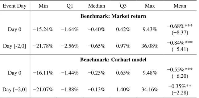
Table I shows statistics on the abnormal returns of the firms in our sample against both benchmarks for � �,�. Using the market return as a benchmark, high-tech firms experienced an average abnormal return of −0.68% on Day 0. Using Carhart’s four-factor model to develop a benchmark expected return for each firm, the average abnormal return was −0.55%. The table shows t-statistics in parentheses for a standard t-test of the null hypothesis that the mean abnormal return is zero. Against both benchmarks, the test rejects this null hypothesis at the 1% level, indicating a significant and adverse impact of the announcement on high-tech firms.
Vox leaked the text of the travel ban on January 25, two days before its official announcement, so it is possible that the adverse impact on stock prices may have begun on January 26.2 Therefore,
we expand our event window to [−2,0] to include the trading days between the leak and the official announcement. We again find significant, abnormal returns for high-tech firms. Using the market return as a benchmark, the average abnormal return over this three-day window was −0.84%, and was −0.35% using Carhart’s four-factor model.
Table I: Abnormal Returns of High-tech Firms
Event Day Min Q1 Median Q3 Max Mean
Benchmark: Market return
Day 0 −15.24% −1.64% −0.40% 0.42% 9.43% −0.68%*** (−8.37)
Day [-2,0] −21.78% −2.56% −0.65% 0.97% 36.08% −0.84%*** (−5.41)
Benchmark: Carhart model
Day 0 −16.11% −1.44% −0.25% 0.65% 9.48% −0.55%*** (−6.20)
Day [−2,0] −21.07% −1.88% −0.13% 1.40% 34.16% −0.35%** (−2.28)
Notes: Table gives the average abnormal returns for �= 616 high-tech firms in our sample. Day 0 is the first trading day after the announcement of the travel ban. T-statistic in parentheses is for the test of the null hypothesis that the mean abnormal return is zero. ***, ** and * indicate significance at 10%, 5% and 1% respectively.
In examining these results, it is worth noting that the abnormal losses over the event window
[−2,0] are larger than the Day 0 losses using the market return as a benchmark, but smaller than the Day 0 losses using the Carhart model, suggesting an inconsistency on days [−2,−1] . President Trump’s first week in office was extremely active. For example, on January 25, he signed Executive Order 13767, directing the construction of a wall along the Mexican border. On January 26, he cancelled a high-profile meeting with Mexican president Enrique Peña Nieto. With this in mind, a potential explanation for the discrepancy in our results is that the Carhart model controls for firm-specific size and growth factors. That is, other intervening events on days [−2,−1] likely affected large firms and small firms differently. In particular, instability in our relationship with major trading partners has a stronger effect on the operating costs of large firms that rely heavily on international supply chains, and this firm size effect could drive the inconsistency in our results. To test this claim, we removed the size factor from the Carhart model and re-estimated the abnormal returns. In this case, the average abnormal return over event days [−2,−1] changes to negative and significant, consistent with the market return benchmark, and thus consistent with our explanation that firm size effects drive the difference in results.
3.2Drivers of Abnormal returns
Having established the existence of abnormal returns for high-tech companies on the first trading day after the travel ban was announced, we now examine how these losses in stock value varied across the firms in our sample.
First, firms with greater R&D intensity experienced larger losses. Measuring R&D intensity as R&D expense divided by total asset value, we find preliminarily that firms in the top half of the distribution of R&D intensity experienced an average abnormal return of −0.96% on the first trading day following the announcement, versus an average of −0.13% for the firms with lower R&D intensity.3 The difference is significant at the 1% level.
Second, global firms experienced smaller losses. We define a global firm as a company that has at least one business segment outside of the United States, as identified in Compustat. Our sample includes 416 global firms and 200 firms with strictly domestic operations. Using Carhart’s four-factor model for the benchmark return, the global firms experienced an average abnormal return of −0.11% on the first trading day following the announcement. By contrast, firms without an international segment experienced an average abnormal return of −1.45%. The difference is significant at the 1% level.
To explore these associations more robustly, we regress the abnormal return of each firm � on its R&D intensity, a dummy variable reflecting whether the firm is a global firm with an international segment, and a vector of firm characteristics ��.
� � = + ⋅(R&D Intensity�) + ⋅(Global�) + �� +��
Our firm-specific controls � include the logarithm of total assets, financial leverage (total debt divided by total assets), profitability (return on equity), and to-market ratio. ROE and book-to-market ratio are winsorized at the 2.5 and 97.5 percentiles to adjust for outliers. We also control
3 These averages use Carhart’s four-factor model for the benchmark. Results are similar using the market return as a
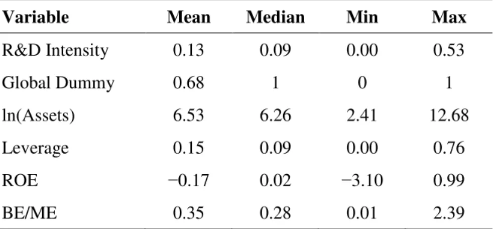
for industry fixed effects (based on 3-digit SIC). Table II gives descriptive statistics on all firm characteristics.
Table II: Descriptive Statistics
Variable Mean Median Min Max
R&D Intensity 0.13 0.09 0.00 0.53
Global Dummy 0.68 1 0 1
ln(Assets) 6.53 6.26 2.41 12.68
Leverage 0.15 0.09 0.00 0.76
ROE −0.17 0.02 −3.10 0.99
BE/ME 0.35 0.28 0.01 2.39
Notes: R&D intensity is R&D expenditures divided by total assets. Global is a dummy equal to 1 if the firm has at least one segment outside of the US. ln(Assets) is the natural log of the firm’s assets. Leverage is total debt divided by total assets. ROE is earnings divided by last year’s book value of equity. BE/ME is book value (stockholder equity plus balance sheet deferred taxes and investment tax credit minus book value of preferred stock) divided by market value of equity. ROE and BE/ME are winsorized at the 2.5 and 97.5 percentiles.
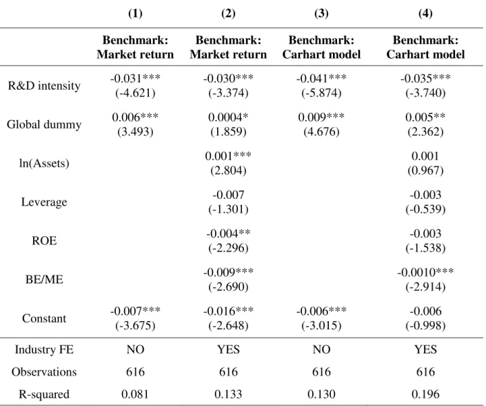
Table III gives the results from these regressions. Models (1) and (2) use the market return as the benchmark for abnormal returns, without and with firm-specific controls respectively. Models (3) and (4) use Carhart’s four-factor model as the benchmark, again without and with controls respectively. Consistent with the descriptive results above, our estimates of are negative and significant at the 1% level in all four models, reflecting larger losses for firms with greater R&D intensity. Conversely, our estimates of are positive, reflecting a mitigation of losses for firms with an international segment. Estimates of are significant at the 5% level in all but model (2), where the coefficient estimate is significant at the 10% level.
To interpret these coefficients, consider model (4), using Carhart’s four-factor model and including all firm-specific controls. The coefficient estimates suggest that a firm with R&D intensity at the sample median level of 9% would have been expected to experience abnormal losses 0.32% larger than those of a firm with no R&D expenditures.4 On the other hand, the
average abnormal losses of a global firm were 0.50% smaller than those of a firm without an international segment, all else equal.
An interesting feature of our results is that the coefficient on book value divided by market value of equity (BE/ME) is negative and significant in both model (2) and model (4), which suggests that value firms experienced larger price drops than growth firms. This finding is consistent with results from the existing literature that value stocks are fundamentally riskier than
4 Each 1% increase in R&D intensity is associated with a 0.035% larger abnormal loss, and the median firm’s R&D
growth stocks and that they exhibit a larger response to economic shocks (Petkova and Zhang 2005; Choi 2013).
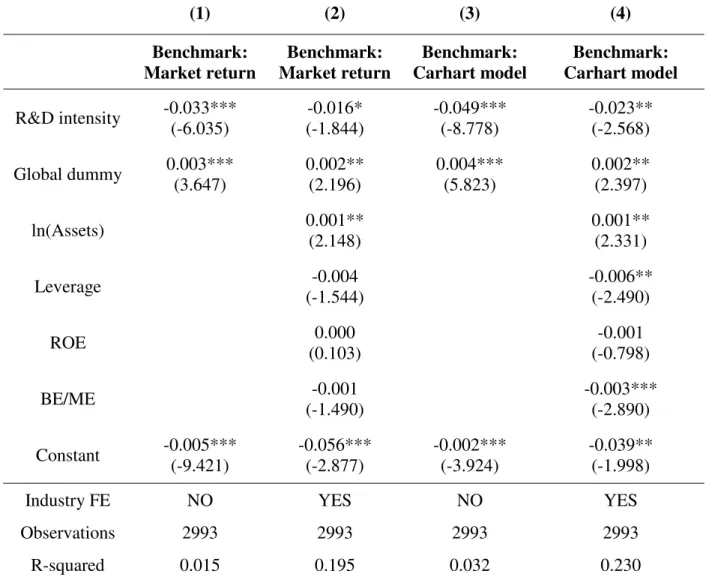
Finally, we check whether the same basic result holds for all firms listed on the stock exchange. To do this, we repeat our analysis, but with all firms listed on NYSE, NASDAQ or AMEX that satisfy the criteria outlined in section 2.2 other than the condition that the firm operate in a high-tech industry. This increases the sample size from 616 firms to 1,993 firms. The results are given in Table IV. The directional results are the same – Firms with higher R&D intensity experienced larger losses, but losses were mitigated for global firms. However, using our robust models with firm-specific controls, these effects are much stronger for high-tech firms than they are for all firms listed on the exchange. In other words, the factors we are studying are qualitatively more important in explaining the exposure of high-tech firms to this shock than they are for other firms on the market.
Together, our results suggest that the potential for the travel ban to damage R&D capacity drove the abnormal losses of high-tech firms. These firms rely on skilled immigrants to relieve a domestic shortage of skilled workers and researchers (Ozden and Schiff 2005), so it is unsurprising that capital markets reacted negatively with respect to these firms on the announcement of new restrictions on the movement of labor and skills. However, our results also suggest that global firms have more readily available options for alleviating the impact of these restrictions. For example, a firm with an international segment could move a skilled worker to an overseas branch in order to keep him in the company, an option not available to domestic firms.
4.
Conclusion
Table III: Determinants of Abnormal Returns of High-tech Firms
(1) (2) (3) (4)
Benchmark: Market return Benchmark: Market return Benchmark: Carhart model Benchmark: Carhart model
R&D intensity -0.031*** (-4.621) -0.030*** (-3.374) -0.041*** (-5.874) -0.035*** (-3.740)
Global dummy 0.006*** (3.493) 0.0004* (1.859) 0.009*** (4.676) 0.005** (2.362)
ln(Assets) 0.001***
(2.804)
0.001 (0.967)
Leverage -0.007
(-1.301)
-0.003 (-0.539)
ROE -0.004**
(-2.296)
-0.003 (-1.538)
BE/ME -0.009***
(-2.690)
-0.0010*** (-2.914)
Constant -0.007*** (-3.675) -0.016*** (-2.648) -0.006*** (-3.015) -0.006 (-0.998)
Industry FE NO YES NO YES
Observations 616 616 616 616
R-squared 0.081 0.133 0.130 0.196
Table IV: Determinants of Abnormal Returns of All Firms on Exchange
(1) (2) (3) (4)
Benchmark: Market return Benchmark: Market return Benchmark: Carhart model Benchmark: Carhart model
R&D intensity -0.033*** (-6.035) -0.016* (-1.844) -0.049*** (-8.778) -0.023** (-2.568)
Global dummy 0.003*** (3.647) 0.002** (2.196) 0.004*** (5.823) 0.002** (2.397)
ln(Assets) 0.001**
(2.148)
0.001** (2.331)
Leverage -0.004
(-1.544)
-0.006** (-2.490)
ROE 0.000
(0.103)
-0.001 (-0.798)
BE/ME -0.001
(-1.490)
-0.003*** (-2.890)
Constant -0.005*** (-9.421) -0.056*** (-2.877) -0.002*** (-3.924) -0.039** (-1.998)
Industry FE NO YES NO YES
Observations 2993 2993 2993 2993
R-squared 0.015 0.195 0.032 0.230
References
Austin, D. H. (1993) “An event-study approach to measuring innovative output: The case of biotechnology” The American Economic Review83, 253-258.
Brown, J. R., Fazzari, S. M. and B. C. Petersen (2009) “Financing innovation and growth: Cash flow, external equity, and the 1990s R&D boom” The Journal of Finance64, 151-185.
Carhart, M. M. (1997) “On persistence in mutual fund performance” The Journal of Finance52, 57-82.
Chang, E. C., Cheng, J. W. and Y. Yu (2007) “Short‐sales constraints and price discovery: Evidence from the Hong Kong market” The Journal of Finance62, 2097-2121.
Choi, J. (2013) “What drives the value premium? The role of asset risk and leverage” The Review of Financial Studies26, 2845-2875.
Fama, E. F., Fisher, L., Jensen, M. C. and R. Roll (1969) “The adjustment of stock prices to new information” International Economic Review10, 1-21.
Fernando, C. S., May, A. D., and W.L. Megginson (2012) “The value of investment banking relationships: Evidence from the collapse of Lehman Brothers” The Journal of Finance67, 235-270.
Malecki, E. J. (1997) “Technology and economic development: the dynamics of local, regional, and national change”, Retrieved from https://ssrn.com/abstract=1496226
Petkova, R. and L. Zhang (2005) “Is value riskier than growth?” Journal of Financial Economics
78, 187-202.
Ozden, C. and M. Schiff (Eds.) (2006) International Migration, Remittances, and the Brain Drain, The World Bank: Washington DC.
Silver, N. (2017) “Trump is doing what he said he’d do” FiveThirtyEight, Retrieved from https://fivethirtyeight.com/features/trump-is-doing-what-he-said-hed-do/
Zito, S. (2016) “Taking Trump seriously, not literally” The Atlantic, Retrieved from