Fast optimization methods for image registration in adaptive radiation therapy

(1)

Cover Page

The following handle

h

olds various files of this Leiden University dissertation:

http://hdl.handle.net/1887/59448

Author: Qiao, Y.

(2)

Fast optimization methods for image

registration in adaptive radiation

therapy

(3)

Colophon

About the covers:

This is a pathway to find the summit (optimal value).

Fast optimization methods for image registration in adaptive radiation therapy Yuchuan Qiao

ISBN: 978-94-6299-732-5

Thesis layout & cover designs by Yuchuan Qiao Printed by Ridderprint BV

(4)

Fast optimization methods for image

registration in adaptive radiation

therapy

Proefschrift

ter verkrijging van

de graad van Doctor aan de Universiteit Leiden,

op gezag van Rector Magnificus prof.mr. C.J.J.M. Stolker,

volgens besluit van het College voor Promoties

te verdedigen op woensdag, 1 november, 2017

klokke 10:00 uur

door

Yuchuan Qiao

(5)

Promotor: Prof. dr. ir. B. P. F. Lelieveldt

Co-promotor: Dr. ir. M. Staring

Leden promotiecommissie: Prof. dr. Andrew Webb

Dr M. Hoogeman Erasmus MC, Rotterdam Prof J.P.W. Pluim

Technische Universiteit Eindhoven, Eindhoven

Advanced School for Computing and Imaging

This work was carried out in the ASCI graduate school. ASCI dissertation series number: 377

Financial support for the publication of this thesis was kindly provided by:

• China Scholorship Council (CSC),

• Bontius Stichting,

(6)

1

Introduction

1.1 Medical image registration

Medical imaging has become an indispensable tool in health care for diagnosis, treatment planning and therapy monitoring. In many cases, medical images are acquired at different stages of the diagnosis and treatment chain. However, medical imaging data is often very heterogenous, in that it can be acquired at different time points (to monitor disease course), or at different imaging devices (providing complementary information). In many cases, the anatomical structures in the images may move or deform due to internal movement (e.g. breathing, bladder filling or cardiac motion) or external function differences between imaging modalities. Also, in studies across multiple subjects, the anatomical structures of different subjects may also differ a lot due to inter-individual differences. The main goal of medical image registration is to find the spatial connection between heterogeneous images or populations.

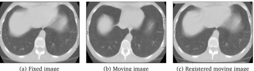
With the increasing use of medical imaging in routine clinical care, medical image registration is an important driver for the development of innovative image analysis technologies. Application examples are CT screening for lung cancer, atlas-based segmentation and image-guided interventions [1, 2, 3]. For instance, in CT screening for lung cancer, follow-up CT scans of the same subject are compared against a

(a) Fixed image (b) Moving image (c) Registered moving image

(11)

(a) CT image (b) MRI image (c) Registered image

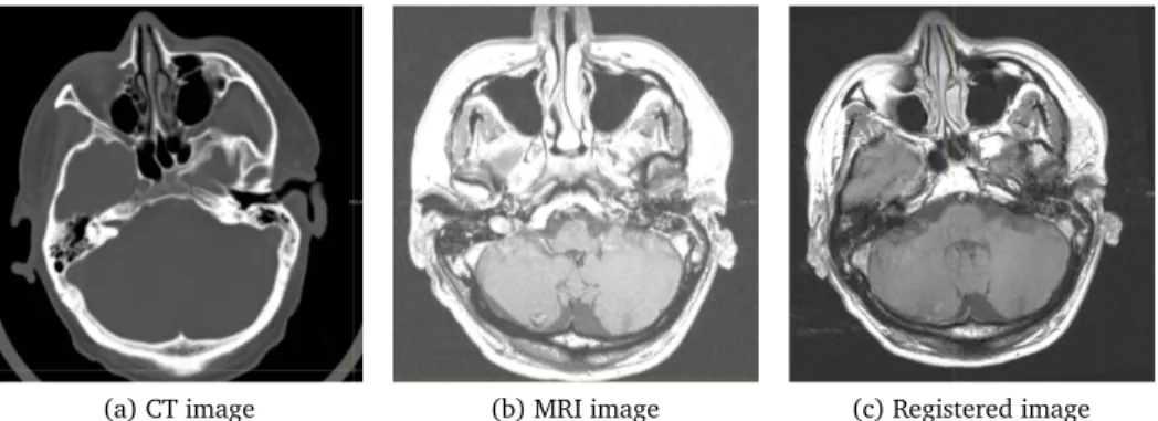
Figure 1.2: Example of CT-MRI registration for target-volume delineation of brain tumors.

baseline CT scan, and a comparison is performed to assess the tumor changes. Even though lung CT scans are acquired at more or less standardized respiration stages, the deformations of the lung can be large. It is essential to register the CT scans to investigate the tumor development in the lung with respect to normal tissues. Figure 1.1 shows an example of deformable image registration to register a follow-up lung CT scan to a baseline CT scan. Besides mono-modal image registration, multi-modal image registration is also used frequently. For example, it can be used to delineate the target volume of brain tumors for the same patient. An example is shown in Figure 1.2. As CT imaging and MR imaging have different resolution and different tissue contrast properties, image registration could integrate these sources of information and provide a better observation of the tumor size change.

In image-guided interventions, for instance image-guided radiation therapy, a planning CT scan is acquired, based on which a treatment plan is generated. The total dose in the treatment plan is usually delivered in daily fractions. The treatment, in particular proton therapy, is sensitive to daily changes in patient setup, the location and shape of the tumor and target volume, and changes in tissue density along the proton beam path. These changes can be captured with the acquisition of a daily CT scan as shown in Figure 1.3. The induced uncertainties by these changes could dramatically distort the dose distribution compared to the planned dose distribution [4, 5, 6, 7, 8]. To achieve highest possible accuracy, the planned dose distribution need therefore be adjusted for the deformations of the tumors over the course of the treatment, which can be computed by image registration.

(12)

C

H

A

P

T

E

R

1

I

N

T

R

O

D

U

C

T

IO

N

(a) Planning CT image (b) Daily CT image

Figure 1.3: Example of organ motion in the planned dose distribution for IMPT of prostate cancer. The prostate and rectum are delineated and represented as a yellow and red solid line, respectively. The shape change of the prostate can be observed.

complicated cost functions, transformation models and optimization methods. It would therefore be highly desirable to accelerate the procedure of image registration, to enable its use in real-time interventions.

1.2 The image registration framework and acceleration approaches

Many approaches can be applied for image registration, such as feature-based image registration and intensity-based image registration. As intensity-based image registra-tion is widely used and most algorithms are developed based on it, we focus on this type of problem in this thesis.

The procedure of intensity-based image registration can be formulated as a

para-metric optimization problem to minimize the dissimilarity between ad-dimensional

fixed imageIF and moving imageIM:

b

µ=arg min

µ C(IF,IM◦Tµ), (1.1)

in whichTµ(x)is a coordinate transformation parameterized byµ. Often used

dissimi-larity measuresC for intensity-based image registration include mutual information

(MI), normalized correlation (NC) and the mean squared intensity difference (MSD) [1, 2, 3]. To account for rotations, translation, global scaling, shrinking and local deformations that occur in medical images, different transformation models are adopted including the translation transform, affine transform and B-spline transform. In particular, complex local deformation models require more degrees of freedom for the transformation models, and are thus more computationally expensive. Multi-resolution strategies on both the image data and the transformation model, allow for a fast and robust image registration [10].

To solve this registration optimization problem, the following iterative scheme is commonly used:

(13)

wherekis the iteration number,γkis the step size at iterationk, anddkis the search

direction in the parameter space. For fast registration methods the search directiondk

as well as the estimation of the step sizeγkneed to be performed with high efficiency.

Gradient descent directions are widely used for the search directiondk.

Gradient-type search directions include steep gradient descent, conjugate gradient descent,

Newton gradient descent and theirstochasticvariations. Because of the exponential

growth of data and parameter spaces in the past twenty years, the computational burden eventually became a bottleneck to find the optimal solution. Stochastic variations of these methods are therefore commonly used with its commendable properties: efficient implementation, little computational burden per iteration and overall less computation cost. These type of methods approximate the deterministic gradient by subsampling the fixed image. However, the inherent drawbacks of stochastic gradient methods are its slow convergence rate and unstable oscillations even if sufficient iterations are provided.

To improve the convergence rate, there are two common approaches. One can use the second order gradient to capture the curvature information of the cost function. A different option is the use of a preconditioning scheme to transform an ill-conditioned cost function to a well-conditioned one at the very beginning of the optimization. Both

are well-known for deterministic gradient type methods. Forstochastictype gradient

methods, the noise in the curvature calculation or the preconditioner estimation may amplify the errors, resulting in a slow convergence rate or a failed registration. Besides this, the calculation of the Hessian or the preconditioner should also be fast, otherwise the gain in the convergence will be lost. New schemes of fast calculation of the Hessian

or the preconditioner forstochastictype gradient methods are therefore needed.

Besides the acceleration schemes in the calculation of the search directiondk, the

selection of the step sizeγk is also important. There are two classes of methods to

determine the step sizeγk: exact and inexact methods. An exact way could be the

conjugate gradient method to determine the step size. An example of an inexact approximation uses for instance a line search method to find the step size that satisfies the Wolfe conditions [11]. However, both schemes are developed for deterministic optimization methods and could not guarantee the convergence of stochastic type methods. For stochastic methods such as stochastic gradient descent, the step size is also an important condition to ensure the convergence, which should meet the following constraints [12, 13, 14, 15],

∞

X

k=1

γk= ∞,

∞

X

k=1

γ2

k < ∞. (1.3)

A common choice for the step size that satisfies this constraint is a monotonically non-increasing sequence. Consider the following decay function for the stochastic methods:

γk=

a

(A+k)α, (1.4)

with a>0, A≥1, 0<α≤1, where α=1 gives a theoretically optimal rate of

convergence [16].

As we can see, in Equation (1.4) the selection of a is important. In medical

(14)

C

H

A

P

T

E

R

1

I

N

T

R

O

D

U

C

T

IO

N

0 200 400 600 800 1000

Runtime (s)

R0 R1 R2 R3

Estimation time Pure registration time

Figure 1.4: An example of runtime in seconds of ASGD for the mutual information measure and a B-spline transformation model. The blue line is the pure registration time and the red line the estimation time of the step size. R0 until R3 are the four resolution levels. The number of transformation parameters for these four resolutions

is around103,104,105and106, respectively. It can be seen that the estimation time

for the step size becomes even larger than the registration time.

and different similarity measures. To select a good step size, the magnitude of a

should be not too large, otherwise the estimated optimal value of cost function will be "bouncing", and not too small, otherwise the convergence will be slow [17, 18].

Choosing a suitable step size therefore is difficult to perform manually. Klein et

al. [15] proposed a method to automatically estimate the step size for adaptive

stochastic gradient descent (ASGD) by considering the distribution of transformations. This method works for few parameters within a reasonable time, but for a large

number of transformation parameters, i.e. in the order of105or higher, the runtime

is unacceptable and the time used in estimating the step size will dominate the optimization procedure. An example to illustrate this limitation is given in Figure 1.4. This limitation disqualifies ASGD for real-time image registration tasks. A fast alternative is therefore needed for real-time registration problems.

1.3 Outline of the thesis

The aim of this thesis is to develop novel optimization strategies for fast image registra-tion. In particular, we address the following specific aims: 1) to investigate strategies to determine the step-size and search direction to accelerate image registration; 2) to develop new stochastic schemes for second order gradient optimization methods; 3) to investigate a new time-efficient preconditioner for preconditioned gradient descent optimization; 4) to validate these novel fast image registration techniques in the context of online adaptive image-guided radiation therapy. The thesis is further structured as follows:

(15)

ASGD) to automatically determine the step size for gradient descent methods, by considering the observed distribution of the voxel displacements between iterations. A relation between the step size and the expectation and variance of the observed distribution is derived. While ASGD has quadratic complexity with respect to the transformation parameters, the fast ASGD method only has linear complexity. Extensive validation has been performed on different datasets with different modalities, inter/intra subjects, different similarity measures and transformation models. To perform a large scale experiment on 3D MR brain data, we have developed efficient and reusable tools to exploit an international high performance computing facility. This method is already integrated in an

open source deformable image registration packageelastix.

Chapter 3 ASGD not only outperforms deterministic gradient descent methods but also quasi-Newton method in terms of runtime. ASGD, however, only exploits first-order information of the cost function. In this chapter, we explore a stochastic quasi-Newton method (s-LBFGS) for non-rigid image registration. It uses the classical limited memory BFGS method in combination with noisy estimates of the gradient. Curvature information of the cost function is estimated

once everyLiterations and then used for the nextLiterations in combination

with a stochastic gradient. The method is validated on follow-up data of 3D chest CT scans (19 patients), using a B-spline transformation model and a mutual information metric.

Chapter 4 In case of ill-conditioned problems, ASGD only exhibits sublinear con-vergence properties. In Chapter 4, we propose an efficient preconditioner estimation method to improve the convergence rate of ASGD. Based on the observed distribution of voxel displacements in the registration, we estimate the diagonal entries of a preconditioning matrix, thus rescaling the optimization cost function. This makes the preconditioner suitable for stochastic as well as for deterministic optimization. It is efficient to compute and can be used for mono-modal as well as multi-modal cost functions, in combination with different transformation models like the rigid, affine and B-spline models.

Chapter 5 In Chapter 5, we have investigated the performance of the method de-veloped in Chapter 2, for fast and robust contour propagation in the context of online-adaptive IMPT for prostate cancer. The planning CT scan and 7-10 repeat CT scans of 18 prostate cancer patients were used in this study. Automatic contour propagation of repeat CT scans was performed and compared with manual delineations in terms of geometric accuracy and runtime. Dosimetric accuracy was quantified by generating IMPT plans using the propagated contours expanded with a 2-mm (prostate) and 3.5-mm margin (seminal vesicles and lymph nodes) and calculating coverage based on the manual delineation. A

coverage ofV95%≥98%was considered clinically acceptable.

(16)

C

H

A

P

T

E

R

2

F

A

S

T

A

U

T

O

M

A

T

IC

S

T

E

P

S

IZ

E

S

T

IM

A

T

IO

N

2

Fast Automatic Step Size Estimation for

Gradient Descent Optimization of Image

Registration

This chapter was adapted from:

Y. Qiao, B. van Lew, B.P.F. Lelieveldt and M. Staring. Fast Automatic Step Size

(17)

Abstract

Fast automatic image registration is an important prerequisite for image guided clinical procedures. However, due to the large number of voxels in an image and the complexity of registration algorithms, this process is often very slow. Among many classical optimization strategies, stochastic gradient descent is a powerful method to iteratively solve the registration problem. This procedure relies on a proper selection of the optimization step size, which is important for the optimization procedure to converge. This step size selection is difficult to perform manually, since it depends on the input data, similarity measure and transformation model. The Adaptive Stochastic Gradient Descent (ASGD) method has been proposed to automatically choose the step size, but it comes at a high computational cost, dependent on the number of transformation parameters.

In this chapter, we propose a new computationally efficient method (fast ASGD) to automatically determine the step size for gradient descent methods, by considering the observed distribution of the voxel displacements between iterations. A relation between the step size and the expectation and variance of the observed distribution is derived. While ASGD has quadratic complexity with respect to the transformation parameters, the fast ASGD method only has linear complexity. Extensive validation has been performed on different datasets with different modalities, inter/intra subjects, different similarity measures and transformation models. To perform a large scale experiment on 3D MR brain data, we have developed efficient and reusable tools to exploit an international high performance computing facility. For all experiments, we obtained similar accuracy as ASGD. Moreover, the estimation time of the fast ASGD method is reduced to a very small value, from 40 seconds to less than 1 second when

the number of parameters is 105_{, almost 40 times faster. Depending on the registration}

(18)

C

H

A

P

T

E

R

2

F

A

S

T

A

U

T

O

M

A

T

IC

S

T

E

P

S

IZ

E

S

T

IM

A

T

IO

N

2.1 Introduction

Image registration aims to align two or more images and is an important technique in the field of medical image analysis. It has been used in clinical procedures including radiotherapy and image-guide surgery, and other general image analysis tasks, such as automatic segmentation [19, 2, 3, 20]. However, due to the large number of image voxels, the large amount of transformation parameters and general algorithm complexity, this process is often very slow [13]. This renders the technique impractical in time-critical clinical situations, such as intra-operative procedures.

To accelerate image registration, multiple methods have been developed targeting the transformation model, the interpolation scheme or the optimizer. Several studies investigate the use of state-of-the-art processing techniques exploiting multi-threading on the CPU or also the GPU [21, 22]. Others focus on the optimization scheme that is used for solving image registration problems [23, 24, 25]. Methods include gradient descent [26, 27], Levenberg-Marquardt [28, 29], quasi-Newton [30, 31], conjugate gradient descent [25], evolution strategies [32], particle swarm methods [33, 34], and stochastic gradient descent methods [35, 15]. Among these schemes, the stochastic gradient descent method is a powerful method for large scale optimization problems and has a superb performance in terms of computation time, with similar accuracy as deterministic first order methods [25]. Deterministic second order methods gave slightly better accuracy in that study, but at heavily increased computational cost. It may therefore be considered for cases where a high level of accuracy is required, in a setting where real-time performance is not needed.

In this study, we build on the stochastic gradient descent technique to solve the optimization problem of image registration [27]:

b

µ=arg min

µ C(IF,IM◦Tµ), (2.1)

in whichIF(x)is thed-dimensional fixed image,IM(x)is thed-dimensional moving

image,T(x,µ)is a parameterized coordinate transformation, andC the cost function

to measure the dissimilarity between the fixed and moving image. To solve this problem, the stochastic gradient descent method adopts iterative updates to obtain the optimal parameters using the following form:

µk+1=µk−γkg˜k, (2.2)

where k is the iteration number, γk the step size at iteration k, g˜k =gk+²k the

stochastic gradient of the cost function, with the true gradientgk=∂C/∂µkand the

approximation error²k. The stochastic gradient can be efficiently calculated using

(19)

is a non-increasing and non-zero sequence withP∞

k=1γk= ∞and P∞

k=1γ 2

k< ∞[12].

A suitable step size sequence is very important, because a poorly chosen step size will cause problems of estimated value "bouncing" if this step size is too large, or slow convergence if it is too small [17, 18]. Therefore, an exact and automatically estimated step size, independent of problem settings, is essential for the gradient-based optimization of image registration. Note that for deterministic quasi-Newton methods the step size is commonly chosen using an (in)exact line search.

Methods that aim to solve the problem of step size estimation can be categorized in three groups: manual, semi-automatic, and automatic methods. In 1952, Robbins and Monro [12] proposed to manually select a suitable step size sequence. Several methods were proposed afterwards to improve the convergence of the Robbins-Monro method, which focused on the construction of the step size sequence, but still required manual selection of the initial step size. Examples include Kesten’s rule [39], Gaivoronski’s rule [40], and the adaptive two-point step size gradient method [41]. An overview of these methods can be found here [42, 43]. These manual selection methods, however, are difficult to use in the practice, because different applications require different settings. Especially for image registration, different fixed or moving images, different similarity measures or transformation models require a different step size. For example, it has been reported that the step size can differ several orders of magnitude between cost functions [15]. Moreover, manual selection is time-consuming.

Spall [36] used a step size following a rule-of-thumb that the step size times the

magnitude of the gradient is approximately equal to the smallest desired change ofµin

the early iterations. The estimation is based on a preliminary registration, after which the step size is manually estimated and used in subsequent registrations. This manual

procedure is not adaptive to the specific images, depends on the parameterization_µ,

and requires setting an nonintuitive ’desired change’ in_µ.

For the semi-automatic selection, Suri [17] and Brennan [18] proposed to use a

step size with the same scale as the magnitude ofµobserved in the first few iterations

of a preliminary simulation experiment, in which a latent difference of the step size between the preliminary experiment and the current one is inevitable. Bhagalia also used a training method to estimate the step size of stochastic gradient descent optimization for image registration [44]. First, a pseudo ground truth was obtained using deterministic gradient descent. Then, after several attempts, the optimal step size was chosen to find the optimal warp estimates which had the smallest error values compared with the pseudo ground truth warp obtained in the first step. This method is complex and time-consuming as it requires training data, and moreover generalizes training results to new cases.

The Adaptive Stochastic Gradient Descent method (ASGD) [15] proposed by Klein et al. automatically estimates the step size. ASGD estimates the distribution of the gradients and the distribution of voxel displacements, and finally calculates the initial step size based on the voxel displacements. This method works for few parameters within reasonable time, but for a large number of transformation parameters, i.e. in

the order of105or higher, the run time is unacceptable and the time used in estimating

the step size will dominate the optimization [45]. This disqualifies ASGD for real-time image registration tasks.

(20)

C

H

A

P

T

E

R

2

F

A

S

T

A

U

T

O

M

A

T

IC

S

T

E

P

S

IZ

E

S

T

IM

A

T

IO

N

descent optimization, by deriving a relation with the observed voxel displacement. This chapter extends a conference chapter [45] with detailed methodology and exten-sive validation, using many different datasets of different modality and anatomical structure. Furthermore, we have developed tools to perform extensive validation of our method by interfacing with a large international computing facility. In Section 2.2, the method to calculate the step size is introduced. The dataset description is given in Section 2.3. The experimental setup to evaluate the performance of the new method is presented in Section 2.4. In Section 2.5, the experimental results are given. Finally, Section 2.6 and 2.7 conclude the chapter.

2.2 Method

A commonly used choice for the step size estimation in gradient descent is to use a monotonically non-increasing sequence. In this chapter we use the following decaying function, which can adaptively tune the step size according to the direction and magnitude of consecutive gradients, and has been used frequently in the stochastic optimization literature [12, 16, 13, 35, 43, 40, 14, 42, 15]:

γk=

a

(A+tk)α

, (2.3)

with a_>0, A_≥1, 0_<α_≤1, where α=1 gives a theoretically optimal rate of

convergence [16], and is used throughout this chapter. The iteration number is

denoted by k, and tk =max(0,tk−1+f(−g˜_kT₋₁g˜k−2)). The function f is a sigmoid

function with f(0)₌0:

f(x)= fmax−fmin

1−(fmax/fmin)e−x/ω+

fmin, (2.4)

in which fmaxdetermines the maximum gain at each iteration, fmin determines the

maximal step backward in time, andωaffects the shape of the sigmoid function [15].

A reasonable choice for the maximum of the sigmoid function isfmax=1, which implies

that the maximum step forward in time equals that of the Robbins-Monro method

[15]. It has been proven that convergence is guaranteed as long astk≥0[14, 15].

Specifically, from Assumption A4 [14] and Assumption B5 [15], asymptotic normality

and convergence can be assured when fmax> −fmin and ω>0. In [15] (Equation

(59))ω=ζqV ar(εT_kεk−1)was used, which requires the estimation of the distribution

of the approximation error for the gradients, which is time consuming. Moreover, a

parameterζis introduced which was empirically set to 10%. Settingω=10−8avoids a

costly computation, and still guarantees the conditions required for convergence. For

the minimum of the sigmoid function we choose fmin= −0.8in this chapter, fulfilling

the convergence criteria.

In the step size sequence {γk}, all parameters need to be selected before the

optimization procedure. The parameterαcontrols the decay rate; the theoretically

optimal value is 1 [10, 15]. The parameter Aprovides a starting point, which has

most influence at the beginning of the optimization. From experience [10, 15], A₌20

provides a reasonable value for most situations. The parameterain the numerator

determines the overall scale of the step size sequence, which is important but difficult to

(21)

between resolutions (Figure 4 [15]) and for different cost functions (Table 2 [15]). This means that the problem of estimating the step size sequence is mainly determined

bya. In this work, we therefore focus on automatically selecting the parameterain a

less time-consuming manner.

2.2.1 Maximum voxel displacement

The intuition of the proposed step size selection method is that the voxel displacements should start with a reasonable value and gradually diminish to zero. The incremental

displacement of a voxelxj in a fixed image domainΩF between iterationk andk+1

for an iterative optimization scheme is defined as

dk(xj)=T¡xj,µk+1 ¢

−T¡

xj,µk¢,∀xj∈ΩF. (2.5)

To ensure that the incremental displacement between each iteration is neither too

big nor too small, we need to constrain the voxel’s incremental displacement dk

into a reasonable range. We assume that the magnitude of the voxel’s incremental

displacementdk follows some distribution, which has expectationE||dk||and variance

V ar_||dk||, in which k · k is the `2 norm. For a translation transform, the voxel

displacements are all equal, so the variance is zero; for non-rigid registration, the voxel displacements vary spatially, so the variance is larger than zero. To calculate

the magnitude of the incremental displacement||dk||, we use the first-order Taylor

expansion to make an approximation ofdk aroundµk:

dk≈∂

T

∂µ ¡

xj,µk

¢

·¡µk+1−µk

¢ =Jj

¡

µk+1−µk

¢

, (2.6)

in whichJj=∂_∂T_µ

¡ xj,µk

¢

is the Jacobian matrix of sized×|µ|. DefiningMk(xj)=J(xj)gk

and combining with the update ruleµk+1=µk−γkgk,dkcan be rewritten as:

dk(xj)≈ −γkJ(xj)gk= −γkMk(xj). (2.7)

For a maximum allowed voxel displacement, Klein [15] introduced a user-defined

parameterδ, which has a physical meaning with the same unit as the image dimensions,

usually in mm. This implies that the maximum voxel displacement for each voxel

between two iterations should be not larger thanδ: i.ekdk(xj)k ≤δ,∀xj∈ΩF.We can

use a weakened form for this assumption:

P(kdk(xj)k >δ)<ρ, (2.8)

whereρis a small probability value often 0.05. According to the Vysochanskij Petunin

inequality [46], for a random variable X with unimodal distribution, meanµand

finite, non-zero varianceσ2_{, if}_λ_>p_(8/3)_{, the following theorem holds:}

P(|X−µ| ≥λσ)≤ 4

9λ2. (2.9)

This can be rewritten as:

(22)

C H A P T E R 2 F A S T A U T O M A T IC S T E P S IZ E E S T IM A T IO N

Based on this boundary, we can approximate Equation (2.8) with the following expression:

E° °d_k(x_j)

° °+2

q V ar°

°d_k(x_j) °

°≤δ. (2.11)

This is slightly different from the squares used in Equation (42) in [15], which avoids taking square roots for performance reasons. In this chapter we are interested in the incremental displacements, not its square. Combining with Equation (2.7), we obtain the relationship between step size and maximum voxel displacement as follows:

γk

µ

E°°M_k(xj)

° °+2

q

V ar°°M_k(xj)

° ° ¶

≤δ. (2.12)

2.2.2 Maximum step size for deterministic gradient descent

From the step size functionγ(k)=a/(k+A)α,it is easy to find the maximum step size

γmax=γ(0)=a/Aα, and the maximum value ofa, amax=γmaxAα. This means that

the largest step size is taken at the beginning of the optimization procedure for each

resolution. Using Equation (2.12), we obtain the following equation ofamax:

amax= δ

Aα

E_kM0(xj)k +2pV arkM0(xj)k

. (2.13)

For a given_δ, the value ofacan be estimated from the initial distribution ofM0at the

beginning of each resolution.

2.2.3 Noise compensation for stochastic gradient descent

The stochastic gradient descent method combines fast convergence with a reasonable accuracy [25]. Fast estimates of the gradient are obtained using a small subset of the fixed image voxels, randomly chosen in each iteration. This procedure introduces noise to the gradient estimate, thereby influencing the convergence rate. This in turn means

that the optimal step size forstochasticgradient descent will be different compared

todeterministicgradient descent. When the approximation error_²₌g−g˜increases,

the search directiong˜ is more unpredictable, thus a smaller and more careful step

size is required. Similar to [15] we assume that²is a zero mean Gaussian variable

with small variance, and we adopt the ratio between the expectation of the exact and

approximated gradient to modify the step sizeamaxas follows:

η=Ekgk 2

Ekg˜k2=

Ekgk2

Ekgk2₊_E_k²k2. (2.14)

2.2.4 Summary and implementation details

2.2.4.1 The calculation ofamaxfor exact gradient descent

The cost function used in voxel-based image registration usually takes the following form:

C(µ)= 1 |ΩF|

X

xj∈ΩF Ψ¡

(23)

in whichΨis a similarity measure,ΩF is a discrete set of voxel coordinates from the

fixed image and|ΩF|is the cardinality of this set. The gradientg of this cost function

is:

g=∂C

∂µ=

1

|ΩF|

X

xj∈ΩF

∂T0

∂µ

∂IM

∂x

∂Ψ

∂IM

. (2.16)

The reliable estimate of amax relies on the calculation of the exact gradient. We

obtain a trade-off between the accuracy of computingg with its computation time,

by randomly selecting a sufficiently large number of samples from the fixed image.

Specifically, to compute (2.16) we use a subsetΩ1

F⊂ΩFof sizeN1equal to the number

of transformation parametersP= |µ|.

Then,Jj=∂_∂T_µ

¡ xj,µk

¢

is computed at each voxel coordinatexj∈Ω1F. The

expecta-tion and variance of_kM0(xj)kcan be calculated using the following expressions:

E_kM0(xj)k = 1

N1 X

xj∈Ω1F

kM0(xj)k, (2.17)

V ar_kM0(xj)k =_N₁1₋₁

X

xj∈Ω1F ¡

kM0(xj)k −EkM0(xj)k

¢2

. (2.18)

2.2.4.2 The calculation ofη

The above analysis reveals that the noise compensation factorηalso influences

the initial step size. This factor requires computation of the exact gradient g and

the approximate gradientg˜. Because the computation of the exact gradient using

all voxels is too slow, uniform sampling is used, where the number of samples is

determined empirically asN2=min(100000,|ΩF|). To obtain the stochastic gradientg˜,

we perturbµby adding Gaussian noise and recompute the gradient, as detailed in

[15].

2.2.4.3 The final formula

The noise compensated step size is obtained using the following formula:

a=η δA

α

E_kM0(xj)k +2pV arkM0(xj)k

. (2.19)

In summary, the gradientg is first calculated using Equation (2.16), and then the

magnitudeM0(xj)is computed at each voxelxj, finally amaxis obtained. In step 2,

the noise compensationηis calculated through the perturbation process. Finally,ais

obtained through Equation (2.19).

2.2.5 Performance of proposed method

In this section, we compare the time complexity of the fast ASGD method with the ASGD method. Here we only give the final formula of the ASGD method, for more details see reference [15]. The ASGD method uses the following equation:

amax=δ

Aα

σ xminj∈Ω1_F h

Tr(JjC J0_j)+2

p

2kJjC J0_jkF

i−1₂

(24)

C

H

A

P

T

E

R

2

F

A

S

T

A

U

T

O

M

A

T

IC

S

T

E

P

S

IZ

E

S

T

IM

A

T

IO

N

whereσis a scalar constant related to the distribution of the exact gradientg [15],

C=_|Ω11 F|2

P

jJ0_jJj is the covariance of the Jacobian, andk · kF denotes the Frobenius

norm.

From Equation (2.13), the time complexity of FASGD is dominated by three terms:

the JacobianJ(xj)with sized×P, the gradientg of sizeP, and the number of voxelsN1

from which the expectation and variance ofM0are calculated. The matrix computation

M0(xj)=J(xj)grequiresd×Pmultiplications and additions for each of theN1voxelsxj,

and therefore the time complexity of the proposed method isO(d N1P). The dominant

terms in Equation (2.20) are the Jacobian (sized×P) and its covariance matrixC

(sizeP_×P). Calculating JjC J0_j from right to left requiresd×P2multiplications and

additions forC J0

j and an additionald

2

×P operations for the multiplication with the

left-most matrixJj. Taking into account the number of voxelsN1, the time complexity

of the original ASGD method is thereforeO(N1×(d×P2+d2×P))=O(d N1P2), asPÀd.

This means that FASGD has a linear time complexity with respect to the dimension of

µ, while ASGD is quadratic inP.

For the B-spline transformation model, the size of the non-zero part of the Jacobian

is much smaller than the full Jacobian, i.e. onlyd_×P2, whereP2is determined by the

B-spline order used in this model. For a cubic B-spline transformation model, each

voxel is influenced by4dcontrol points, soP2=42=16in 2D andP2=43=64in 3D. For

the fast ASGD method the time complexity reduces toO(d N1P2)for the cubic B-spline

model. However, as the total number of operations for the calculation ofJjC J0_j is still

d×P2×P, the time complexity of ASGD is O(d N1P2P). SincePÀN1≥P2>d, the

dominant term of FASGD becomes the number of samplesN1, while for ASGD it is still

a potentially very large numberP.

2.3 Data sets

In this section we describe the data sets that were used to evaluate the proposed method. Data sets were chosen to represent a broad category of use cases, i.e. mono-modal and multi-modal, intra-patient as well as inter-patient, from different anatomical sites, and having rigid as well as nonrigid underlying deformations. The overview of all data sets is presented in Table 2.1.

2.3.1 RIRE brain data – multi-modality rigid registration

The Retrospective Image Registration Evaluation (RIRE) project provides multi-modality brain scans with a ground truth for rigid registration evaluation [47]. These brain scans were obtained from 9 patients, where we selected CT scans and MR T1 scans. Fiducial markers were implanted in each patient, and served as a ground truth. These markers were manually erased from the images and replaced with a simulated background pattern.

In our experiments, we registered the T1 MR image (moving image) to the CT image (fixed image) using rigid registration. At the website of RIRE, eight corner points of both CT and MR T1 images are provided to evaluate the registration accuracy.

2.3.2 SPREAD lung data – intra-subject nonrigid registration

During the SPREAD study [48], 3D lung CT images of 19 patients were scanned without contrast media using a Toshiba Aquilion 4 scanner with scan parameters: 135

(25)

(26)

C

H

A

P

T

E

R

2

F

A

S

T

A

U

T

O

M

A

T

IC

S

T

E

P

S

IZ

E

S

T

IM

A

T

IO

N

reconstructed with a standardized protocol optimized for lung densitometry, including a soft FC12 kernel, using a slice thickness of 5 mm and an increment of 2.5 mm, with

an inplane resolution of around 0.7×0.7 mm. The patient group, aging from 49 to

78 with 36%-87% predicted FEV1had moderate to severe COPD at GOLD stage II and

III, withoutα1antitrypsin deficiency.

One hundred anatomical corresponding points from each lung CT image were semi-automatically extracted as a ground truth using Murphy’s method [49]. The algorithm automatically finds 100 evenly distributed points in the baseline, only at characteristic locations. Subsequently, corresponding points in the follow-up scan are predicted by the algorithm and shown in a graphical user interface for inspection and possible correction. More details can be found in [50].

2.3.3 Hammers brain data – inter-subject nonrigid registration

We use the brain data set developed by Hammerset al. [51], which contains MR

images of 30 healthy adult subjects. The median age of all subjects was 31 years

(range20_∼54), and 25 of the 30 subjects were strongly right handed as determined

by routine pre-scanning screening. MRI scans were obtained on a 1.5 Tesla GE Sigma Echospeed scanner. A coronal T1 weighted 3D volume was acquired using an inversion recovery prepared fast spoiled gradient recall sequence (GE), TE/TR/NEX 4.2 msec (fat and water in phase)/15.5 msec/1, time of inversion (TI) 450 msec, flip angle

20Âˇr, to obtain 124 slices of 1.5 mm thickness with a field of view of18×24cm with a

192×256matrix [52]. This covers the whole brain with voxel sizes of0.94×0.94×1.5

mm3_{. Images were resliced to create isotropic voxels of}_0.94_×_0.94_×_0.94_mm3_{, using}

windowed sinc interpolation.

Each image is manually segmented into 83 regions of interest, which serve as a ground truth. All structures were delineated by one investigator on each MRI in turn before the next structure was commenced, then a separate neuroanatomically trained operator evaluated each structure to ensure that consensus was reached for the difficult cases. In our experiment, we performed inter-subject registration between all patients. Each MR image was treated as a fixed image as well as a moving image, so the total number of registrations for 30 patients was 870 for each particular parameter setting.

2.3.4 Ultrasound data – 4D nonrigid registration

We used the 4D abdominal ultrasound dataset provided by Vijayanet al.[53], which

contains 9 scans from three healthy volunteers at three different positions and angles. Each scan was taken over several breathing cycles (12 seconds per cycle). These scans were performed on a GE Healthcare vivid E9 scanner by a skilled physician using an active matrix 4D volume phased array probe.

The ground truth is 22 well-defined anatomical landmarks, first indicated in the first time frame by the physician who acquired the data, and then manually annotated in all 96 time frames by engineers using VV software [54].

2.4 Experiment setup

(27)

2.4.1 Experimental setup

The experiments focus on the properties of the fast ASGD method in terms of registration accuracy, registration runtime and convergence of the algorithm. We will compare the proposed method with two variants of the original ASGD method.

While for FASGD fminandωare fixed, the ASGD method automatically estimates them.

For a fair comparison, a variant of the ASGD method is included in the comparison,

that sets these parameters to the same value as FASGD: fmin= −0.8andω=10−8. In

summary, three methods are compared in all the experiments: the original ASGD method that automatically estimates all parameters (ASGD), the ASGD method with

default settings only estimatinga(ASGD0_{) and the fast ASGD method (FASGD). The}

fast ASGD method has been implemented using the C++ language in the open

source image registration toolboxelastix[10], where the ASGD method is already

integrated.

To thoroughly evaluate FASGD, a variety of imaging problems including different modalities and different similarity measures are considered in the experiments. Specifi-cally, the experiments were performed using four different datasets, rigid and nonrigid transformation models, inter/intra subjects, four different dissimilarity measures and three imaging modalities. The experiments are grouped by the experimental aim: registration accuracy in Section 2.5.1, registration time in Section 2.5.2 and algorithm convergence in Section 2.5.3. The RIRE brain data is used for the evaluation of rigid registration. The SPREAD lung CT data is especially used to verify the performance of FASGD on four different dissimilarity measures, including the mean squared intensity difference (MSD) [2], normalized correlation (NC) [2], mutual information (MI) [27] and normalized mutual information (NMI) [55]. The Hammers brain data is intended to verify inter-subject registration performance. The ultrasound data is specific for 4-dimensional medical image registration, which is more complex. An overview of the experimental settings is given in Table 2.1.

For the evaluation of the registration accuracy, the experiments on the RIRE brain data, the SPREAD lung CT data and the ultrasound abdominal data, were performed on a local workstation with 24 GB memory, Linux Ubuntu 12.04.2 LTS 64 bit operation system and an Intel Xeon E5620 CPU with 8 cores running at 2.4

GHz. To see the influence of the parameters Aandδon the registration accuracy,

we perform an extremely large scale experiment on the Hammers brain data using

the Life Science Grid (lsgrid) [56], which is a High Performance Computing (HPC)

facility. We tested all combinations of the following settings: A_∈{1.25, 2.5, . . . , 160, 320},

δ∈{0.03125, 0.0625, . . . , 128, 256} (in mm) and k_∈{250, 2000}. This amounts to 252 combinations of registration settings and a total of 657,720 registrations, see Table 2.1. Each registration requires about 15 minutes of computation time, which totals about

164,000 core hours of computation, i.e∼19 years, making the use of an HPC resource

essential. With thelsgridthe run time of the Hammers experiment is reduced to 2-3

days. More details about thelsgridare given in the Appendix.

For a fair comparison, all timing experiments were carried out on the local workstation. Timings are reported for all the registrations, except for the Hammers data set, where we only report timings from a subset. From Equation (2.19), we

know that the runtime is independent of the parametersAandδ. Therefore, for the

(28)

C

H

A

P

T

E

R

2

F

A

S

T

A

U

T

O

M

A

T

IC

S

T

E

P

S

IZ

E

S

T

IM

A

T

IO

N

100 out of the 870 registrations, as a sufficiently accurate approximation.

The convergence of the algorithms is evaluated in terms of the step size, the Euclidean distance error and the cost function value, as a function of the iteration number.

All experiments were done using the following routine: (1) Perform a linear

registration between fixed and moving image to get a coarse transformationT0, using

a rigid transformation for the RIRE brain data, an affine transformation for the SPREAD lung CT data, a similarity transformation rigid plus isotropic scaling for the Hammers brain data, and no initial transformation for the 4D ultrasound data; (2) Perform a non-linear cubic B-spline based registration [57] for all datasets except the RIRE data

to get the transformationT1. For the ultrasound data, the B-spline transformation

model proposed by Metzet al.[58] is used, which registers all 3D image sequences

in a group-wise strategy to find the optimal transformation that is both spatially and temporally smooth. A more detailed explanation of the registration methodology is in

[53]; (3) Transform the landmarks or moving image segmentations usingT1◦T0; (4)

Evaluate the results using the evaluation measures defined in Section 2.4.2.

For each experiment, a three level multi-resolution strategy was used. The Gaussian smoothing filter had a standard deviation of 2, 1 and 0.5 mm for each resolution. For the B-spline transformation model, the grid size of the B-spline control point mesh is halved in each resolution to increase the transformation accuracy [57]. We used

K=500iterations and5000samples, except for the ultrasound experiment where we

used 2000 iterations and 2000 samples according to Vijayan [53]. We set A=20andδ

equal to the voxel size (the mean length of the voxel edges).

2.4.2 Evaluation measures

Two evaluation measures were used to verify the registration accuracy: the Euclidean distance and the mean overlap. The Euclidean distance measure is given by:

ED=1 n

n

X

i=1

kT(p_Fi)−p_Mi k, (2.21)

in whichpi_F andpi_Mare coordinates from the fixed and moving image, respectively.

For the RIRE brain data, 8 corner points and for the SPREAD data 100 corresponding points are used to evaluate the performance. For the 4D ultrasound image, we adopt the following measure from [53]:

ED₌

µ ₁

τ−1

X

t k

pt−Tt(q)k2

¶1₂

, (2.22)

in which pt=1/JPjpt j and pt j is a landmark at time t placed by observer j, q=

1/τP

tSt(pt)is the mean of landmarks after inverse transformation.

The mean overlap of two segmentations from the images is calculated by the Dice Similarity Coefficient (DSC) [13]:

DSC₌ 1

R X

r

2|Mr∩Fr|

|Mr| + |Fr|

, (2.23)

in whichris a labelled region andR₌83the total number of regions for the Hammers

(29)

0 0.5 1 1.5 2

E

D

(m

m

)

ASGD ASGD′ _FASGD

1

Figure 2.1: Euclidean distance error in mm for the RIRE brain data performed using MI.

To assess the registration accuracy, a Wilcoxon signed rank test (p=0.05) for the

registration results was performed. For the SPREAD data, we first obtained the mean distance error of 100 points for each patient and then performed the Wilcoxon signed rank test to these mean errors.

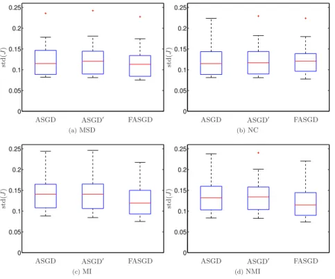
Registration smoothness is assessed for the SPREAD experiment by measuring the

determinant of the spatial Jacobian of the transformation,J_{= |}∂T/∂x|[59]. Because

the fluctuation ofJshould be relatively small for smooth transformations, we use the

standard deviation ofJ to represent smoothness.

The computation time is determined by the number of parameters and the number of voxels sampled from the fixed image. For a small number of parameters the estimation time can be ignored, and therefore we only provide the comparison for the B-spline transformation. Both the parameter estimation time and pure registration time were measured, for each resolution.

2.5 Results

2.5.1 Accuracy results

In this section, we compare the registration accuracy between ASGD, ASGD0 _and

FASGD.

2.5.1.1 RIRE brain data

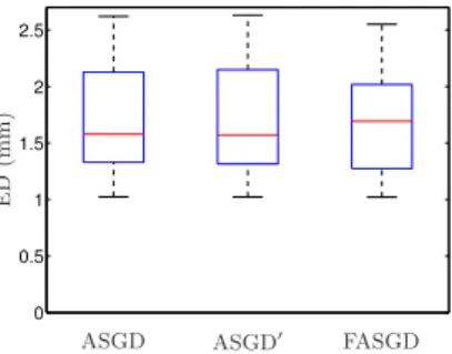
The results shown in Figure 2.1 present the Euclidean distance error of the eight corner points from the brain images. The median Euclidean distance before registration is 21.7 mm. The result of the FASGD method is very similar to the ASGD method: median

accuracy is 1.6, 1.6 and 1.7 mm for ASGD, ASGD0 _{and FASGD, respectively. The}_p

value of the Wilcoxon signed rank test of FASGD compared with ASGD and ASGD0_is

0.36 and 0.30, respectively, indicating no statistical difference.

2.5.1.2 SPREAD lung CT data

(30)

Initial ASGD ASGD0 _FASGD

MSD 3.62 1.09 1.10× 1.12† ‡

NC 3.56 1.50 1.51† 1.55××

MI 3.17 1.65 1.65† 1.66† ‡

NMI 3.17 1.66 1.65× 1.68† ‡

Table 2.2: The median Euclidean distance error (mm) for the SPREAD lung CT data.

The symbols†and‡indicate a statistically significant difference with ASGD and ASGD0_,

respectively.×denotes no significant difference.

−2 −1.5 −1 −0.5 0 0.5 1 1.5

2 ( 0 , 0 ) ( 1 , 0 )

∆ E D (m m )

ASGD′ _FASGD

(a)MSD −2 −1.5 −1 −0.5 0 0.5 1 1.5

2 ( 0 , 0 ) ( 0 , 0 )

∆ E D (m m )

ASGD′ _FASGD

(b)NC −2 −1.5 −1 −0.5 0 0.5 1 1.5

2 ( 0 , 0 ) ( 3 , 1 )

∆ E D (m m )

ASGD′ _FASGD

(c)MI −2 −1.5 −1 −0.5 0 0.5 1 1.5

2 ( 0 , 0 ) ( 8 , 1 )

∆ E D (m m )

ASGD′ _FASGD

(d)NMI

1

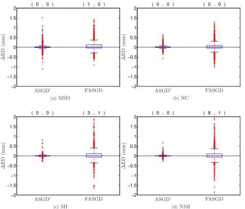
Figure 2.2: The difference of Euclidean distance error in mm compared to ASGD for the SPREAD lung CT data. The two numbers on the top of each box denote the number of the landmark errors larger (left) and smaller (right) than 2 and -2 mm, respectively. All those landmarks, except one for NMI, belong to the same patient.

To compare FASGD and ASGD0_{with ASGD we define the Euclidean landmark error}

difference as∆EDi=EDFASGD_i −EDASGD_i , for each landmarki, and similarly for ASGD0.

This difference is shown as a box plot in Figure 2.2. Negative numbers mean that

FASGD is better than ASGD, and vice versa. It can be seen that both ASGD0_{and FASGD}

provide results similar to ASGD, for all tested cost functions. The spread of the∆ED

box plot for ASGD0_{is smaller than that of FASGD, as this method is almost identical to}

(31)

0 0.05 0.1 0.15 0.2 0.25

ASGD ASGD′ _FASGD

st

d

(

J

)

(a)MSD

0 0.05 0.1 0.15 0.2 0.25

ASGD ASGD′ _FASGD

st

d

(

J

)

(b)NC

0 0.05 0.1 0.15 0.2 0.25

ASGD ASGD′ _FASGD

st

d

(

J

)

(c)MI

0 0.05 0.1 0.15 0.2 0.25

ASGD ASGD′ _FASGD

st

d

(

J

)

(d)NMI

1

Figure 2.3: Box plots of the standard deviation of the Jacobian determinant Jfor the

four similarity measures.

Smoothness of the resulting transformations is given in Figure 2.3 for all similarity measures. FASGD generates somewhat smoother transformations over ASGD and

ASGD0_{for the MSD, MI and NMI measures.}

2.5.1.3 Hammers brain data

In this experiment, FASGD is compared with ASGD and ASGD0 _{in a large scale}

intersubject experiments on brain MR data, for a range of values of A, δ and the

number of iterationsK.

Figure 2.4 shows the overlap results of the 83 brain regions. Each square represents the median DSC result of 870 brain image registration pairs for a certain parameter

combination ofA,δandK. These results show that the original ASGD method has a

slightly higher DSC than FASGD with the same parameter setting, but the median DSC difference is smaller than 0.01. Note that the dark black color indicates DSC values between 0 and 0.5, i.e. anything between registration failure and low performance.

The ASGD and ASGD0_{methods fail for}_δ_≥₃₂_{mm, while FASGD fails for}_δ_≥₂₅₆_mm.

2.5.1.4 Ultrasound Abdomen data

(32)

ASGD, K = 250

A 1.25 2.5 5 10 20 40 80 160 320

ASGD′, K = 250

FASGD, K = 250

ASGD, K = 2000

A

δ[mm]

0.0312 0.0625 0.125 0.25 0.5

1 2 4 8 16 32 64 ₁₂₈ ₂₅₆

1.25 2.5 5 10 20 40 80 160 320

ASGD′, K = 2000

δ[mm]

0.0312 0.0625 0.125 0.25 0.5

1 2 4 8 16 32 64 ₁₂₈ ₂₅₆

FASGD, K = 2000

δ[mm]

0.0312 0.0625 0.125 0.25 0.5

1 2 4 8 16 32 64 ₁₂₈ ₂₅₆

DSC 0.5 0.52 0.54 0.56 0.58 0.6 0.62 0.64 0.66 0.68 0.7

Figure 2.4: Median dice overlap after registration of the Hammers brain data, as a

function ofAandδ. A high DSC indicates better registration accuracy. Note that in

this large scale experiment, each square represents 870 registrations, requiring about

870×15minutes of computation, i.e. almost 200 core hours.

E

D

(m

m

)

ASGD ASGD′ _FASGD

0 1 2 3 4 5 6

Figure 2.5: Euclidean distance in mm of the registration results for Ultrasound data performed using MI.

pvalue of the Wilcoxon signed rank test of FASGD compared with ASGD and ASGD0_is

0.485 and 0.465, respectively, indicating no statistical difference.

2.5.2 Runtime results

In this section the runtime of the three methods, ASGD, ASGD0_{and FASGD is compared.}

(33)

ASGD ASGD′ FASGD R u n ti m e (s ) R1 R1

R1 R2 R3 R2 R3 R2 R3

0 10 20 30 40 50 60 (a) MSD

ASGD ASGD′ FASGD

R u n ti m e (s ) R1 R1

R1 R2 R3 R2 R3 R2 R3

0 10 20 30 40 50 60 (b) NC

ASGD ASGD′ FASGD

R1 R2 R3 R2 R3 R2 R3

0 10 20 30 40 50 60 (c) MI

ASGD ASGD′ FASGD

R1 R2 R3 R2 R3 R2 R3

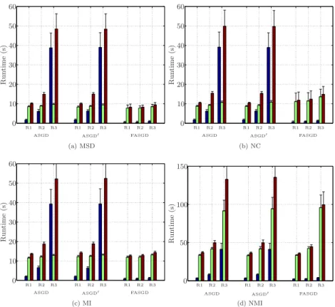
0 50 100 150 (d) NMI 1

Figure 2.6: Runtime of SPREAD lung CT data in seconds. The black, green and red bar indicate estimation time, pure registration time and total time elapsed in each resolution, respectively. R1, R2, R3 indicate a three level multi-resolution strategy from low resolution to high resolution.

2.5.2.1 SPREAD lung CT data

The runtime on SPREAD lung CT data is shown in Figure 2.6, in which the time used in the estimations of the original method takes a large part of the total runtime per resolution, while FASGD consumes only a small fraction of the total runtime. From resolution 1 (R1) to resolution 3 (R3), the number of transformation parameters

P increases from4×103to 9×104. For both ASGD and ASGD0 _{the estimation time}

increases from 3 seconds in R1 to 40 seconds in R3. However, FASGD maintains a constant estimation time of no more than 1 second.

2.5.2.2 Hammers brain data

The runtime result of the Hammers brain data is shown in Figure 2.7. For this dataset,

P_≈1.5_×105in R3, i.e. larger than for the SPREAD data, resulting in larger estimation

times. For ASGD and ASGD0_{the estimation time in the third resolution is almost}₉₅

(34)

C

H

A

P

T

E

R

2

F

A

S

T

A

U

T

O

M

A

T

IC

S

T

E

P

S

IZ

E

S

T

IM

A

T

IO

N

R1 R2 R3 R1 R2 R3 R1 R2 R3 0

20 40 60 80 100 120

ASGD ASGD′ _FASGD

R

u

n

ti

m

e

(s

)

1

Figure 2.7: Runtime of Hammers brain data experiment in seconds. The black, green and red bar indicate estimation time, pure registration time and total time elapsed in each resolution, respectively. R1, R2, R3 indicate a three level multi-resolution strategy from low resolution to high resolution.

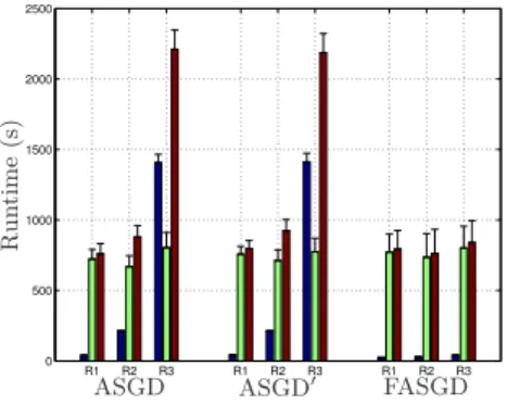
R1 R2 R3 R1 R2 R3 R1 R2 R3 0

500 1000 1500 2000 2500

ASGD ASGD′ _FASGD

R

u

n

ti

m

e

(s

)

1

Figure 2.8: Runtime of Ultrasound data experiment in seconds. The black, green and red bar indicate estimation time, pure registration time and total time elapsed in each resolution, respectively. R1, R2, R3 indicate a three level multi-resolution strategy from low resolution to high resolution.

2.5.2.3 4D ultrasound data

The grid spacing of B-spline control points used in the 4D ultrasound data experiment

is 15_×15_×15_×1 and the image size is227_×229_×227_×96, so the total number of

B-spline parameters for the third resolution R3 is around8.7_×105. From the timing

results in Figure 2.8, the original method takes almost1400seconds, i.e. around 23

minutes, while FASGD only takes 40 seconds.

Figure 2.9 presents the runtime of estimatingamaxandηfor the ultrasound data.

The estimation ofηtakes a constant time during each resolution, so for smallP the

estimation ofηdominates the total estimation time.

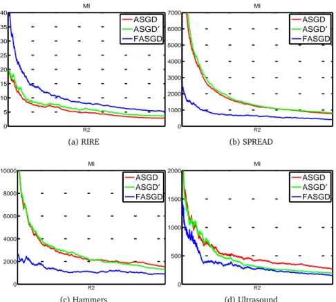
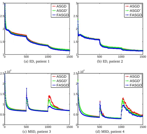
2.5.3 Convergence

From each of the four experiments, we randomly selected one patient and analyzed

Fast optimization methods for image registration in adaptive radiation therapy

Cover Page

The following handle

h

olds various files of this Leiden University dissertation:

http://hdl.handle.net/1887/59448

Author: Qiao, Y.

Fast optimization methods for image

registration in adaptive radiation

therapy

Colophon

Fast optimization methods for image

registration in adaptive radiation

therapy

Proefschrift

ter verkrijging van

de graad van Doctor aan de Universiteit Leiden,

op gezag van Rector Magnificus prof.mr. C.J.J.M. Stolker,

volgens besluit van het College voor Promoties

te verdedigen op woensdag, 1 november, 2017

klokke 10:00 uur

door

Yuchuan Qiao

Contents

1

Introduction

1.1

Medical image registration

1.2

The image registration framework and acceleration approaches

1.3

Outline of the thesis

2

Fast Automatic Step Size Estimation for

Gradient Descent Optimization of Image

Registration

2.1

Introduction

2.2

Method

2.3

Data sets

2.4

Experiment setup

2.5

Results