METHODS FOR POPULATION
PHARMACOKINETICS AND
PHARMACODYNAMICS
Emily Anne Colby
A dissertation submitted to the faculty of the University of North Carolina at Chapel Hill in partial fulfillment of the requirements for the degree of Doctor of Public Health in the Department of Biostatistics.
Chapel Hill 2012
Approved by:
Dr. Eric Bair Gary Koch
c
Abstract
EMILY ANNE COLBY: Methods for Population Pharmacokinetics and Pharmacodynamics
(Under the direction of Dr. Eric Bair)
Current applications of cross validation have been unsuccessful at identifying co-variate effects in the population Pharmacokinetic/Pharmacodynamic (PK/PD) setting when other methods find a covariate effect may exist. Software that does population PK/PD modeling has a nice feature of being able to do a post hoc step without any major iterations to obtain Bayesian parameter estimates and hence predictions for sub-jects that were not in the dataset that was used to fit the model. This work proposes cross validation methods for longitudinal mixed effects models that are effective at identifying covariate effects when they exist.
Acknowledgments
Table of Contents
List of Tables . . . viii
List of Figures . . . ix
1 Introduction and Literature Review . . . 1
1.1 Introduction . . . 1
1.2 Literature Review . . . 2
1.2.1 Background . . . 2
1.2.2 Structure of Population PK/PD Models . . . 3
1.2.3 Population PK/PD Modeling Procedure . . . 8
1.2.4 Challenges in Population PK/PD Modeling . . . 14
1.2.5 Smoothing Splines . . . 15
1.2.6 Cross-Validation . . . 16
1.2.7 Current Uses of Cross-Validation in Population PK/PD . . . 17
1.2.8 Automated Covariate Selection in Population PK/PD . . . 20
1.3 Proposed Research . . . 20
2 Cross validation for Longitudinal Mixed Effects Models . . . 21
2.1 Overview . . . 21
2.2 Introduction . . . 22
2.2.1 Cross-Validation . . . 24
2.3 Methods . . . 25
2.3.1 Comparing models with major structural differences . . . 25
2.3.2 Comparing covariate models . . . 28
2.4 Simulation Example 1 . . . 30
2.5 Simulation Example 2 . . . 33
2.6 Simulation Example 3 . . . 35
2.7 Simulation Example 4 . . . 38
2.8 Simulation Example 5 . . . 42
2.9 Computational details . . . 44
2.10 Simulation Results . . . 45
2.11 Indomethacin Example . . . 49
2.12 Theophylline Example . . . 54
2.13 Discussion . . . 56
3 Automated Model Building Procedure . . . 59
3.1 Overview . . . 59
3.2 Introduction . . . 59
3.3 Methods . . . 61
3.3.1 Comparing covariate models . . . 61
3.3.2 Automated Model Selection Procedure . . . 63
3.4 Remifentanil Example . . . 65
3.5 Simulation Example . . . 68
3.6 Simulation Results . . . 74
3.7 Discussion . . . 76
4 Comparison of Smoothing Splines to Pop PK . . . 77
4.2 Methods . . . 77
4.2.1 Traditional Population Pharmacokinetic Modeling . . . 78
4.2.2 Smoothing Splines . . . 79
4.3 Simulated Data Examples . . . 80
4.4 Results . . . 83
4.5 Real Data Examples . . . 83
4.6 Discussion . . . 85
Appendix . . . 88
Bibliography . . . 96
List of Tables
2.1 Proportion correct out of 200 replicates . . . 46
2.2 Summary of AIC and BIC in simulation scenarios . . . 48
2.3 Summary of nPRESS in simulations . . . 49
2.4 Summary of mPRESS in simulations . . . 50
2.5 Summary of wtmPRESS in simulations . . . 51
2.6 Theta from final model of Indomethacin dataset . . . 52
2.7 Omega from final model of Indomethacin dataset . . . 53
3.1 Theta from final model of Remifentanil dataset . . . 67
3.2 Omega from final model of Remifentanil dataset . . . 68
3.3 Omega for simulation . . . 73
3.4 Models chosen for each replicate . . . 74
3.5 Models chosen for each replicate (cont’d) . . . 75
4.1 Theta from final model of Indomethacin dataset . . . 84
List of Figures
1.1 A three-compartment pharmacokinetic model . . . 5
1.2 Drug concentration versus time for a two-compartment model . . . 11
2.1 Simulation Example 1 data . . . 32
2.2 Simulation Example 2 data, by age quartiles . . . 34
2.3 Simulation Example 3 data, by age quartiles . . . 37
2.4 Simulation Example 4 data, by hepatic impairment . . . 41
2.5 Simulation Example 5 data . . . 44
2.6 Concentration versus time from Indomethacin dataset . . . 52
2.7 Final model of Indomethacin dataset . . . 54
2.8 Residuals from final model of Indomethacin dataset . . . 55
2.9 Observed versus predicted values for Indomethacin model . . . 56
2.10 Concentration versus time from Theophylline dataset . . . 57
2.11 Eta versus covariate plots for Theophylline dataset . . . 58
3.1 Concentration versus time from Remifentanil dataset . . . 65
3.2 Residuals with Additive residual error model . . . 66
3.3 Final model of Remifentanil dataset . . . 69
3.4 Residuals from final model of Remifentanil dataset . . . 69
3.5 Observed versus predicted values from Remifentanil model . . . 70
3.6 Predictive check from final Remifentanil model . . . 70
3.7 Simulated data . . . 73
4.1 Simulated data . . . 80
4.2 Concentration versus time from Indomethacin dataset . . . 84
4.3 Final model of Indomethacin dataset . . . 86
4.4 Residuals from final model of Indomethacin dataset . . . 86
Chapter 1
Introduction and Literature Review
1.1
Introduction
Cross validation has been used in various forms in the population pharmacokinetic (PK) setting. With all the variations, there are two common uses of cross valida-tion currently being used for populavalida-tion Pharmacokinetic/Pharmacodynamic (PK/PD) modeling. Those are final model validation and model comparison.
For model comparison, cross validation has been unsuccessful at finding covariate effects when other methods seem to imply that covariate effects exist (Zomorodi et al., 1998), (Fiset et al., 1995). However, cross validation has been successful at identifying models with major structural differences (Valodia et al., 2000).
First, a review of the literature is presented. Then, the methods are proposed and evaluated using simulated data examples and real data examples.
1.2
Literature Review
This chapter reviews the literature pertaining to population pharmacokinetics and pharmacodynamics.
1.2.1
Background
Population pharmacokinetic and pharmacodynamic (PK/PD) modeling is the char-acterization of the distribution of probable PK/PD outcomes (parameters, concentra-tions, responses, etc.) in a population of interest. These models consist of fixed and random effects. The fixed effects describe the relationship between explanatory vari-ables such as age, body weight, gender, and pharmacokinetic outcomes. The random effects quantify unexplained variation in PK/PD outcomes (FDA, 1999).
Population PK/PD modeling is useful for identifying influential covariates that may warrant some action, such as changes in labeling, dose adjustment, contraindication, and modification of design of future clinical trials. Quantification of unexplained vari-ation in PK may be relevant to assessing safety risks and determining whether dose individualization is desirable or necessary. It can answer questions like “Is it all right to give everyone the same dose, regardless of body weight? If not, how should the doses be scaled?” (FDA, 1999).
There are two approaches to population modeling: the two-stage approach and non-linear mixed effects (NLME) modeling (FDA, 1999). The two-stage approach consists of fitting PK models for each individual separately, then summarizing the PK parameters across individuals. Covariate relationships may be found by regressing the natural log of the PK parameters with covariates of interest. The NLME approach differs in that it fits one model across all individuals. This paper will focus on the NLME approach.
1.2.2
Structure of Population PK/PD Models
Population PK models are hierarchical (Davidian and Giltinan, 1995). There is a model for the individual, a model for the population, and a model for the residual error. The individual model consists of the curve of drug concentrations over time.
To explore the model for the individual, one must have a basic understanding of drug pharmacokinetics. There are four basic phases of drug pharmacokinetics: Absorption, Distribution, Metabolism, and Excretion (ADME). Typically a drug is given as an injection (intravenous), an infusion, or extravascular dose (oral, sublingual, inhalation, patch). Once the drug enters the body, it may undergo an absorptive phase prior to being taken into the plasma. If it is injected as a bolus, this phase does not occur. Once in plasma, the drug is distributed to various organs and tissues. It is often metabolised by an organ such as the liver or kidney, then excreted in urine, feces, or by exhalation. Drug concentration data can be modeled with compartmental modeling, which in-volves curve fitting, or non-compartmental analysis (NCA). Non-compartmental analy-sis conanaly-sists of calculation of pharmacokinetic parameters based on the data alone, with very few assumptions involved. Parameters such as Tmax, the time at which the max-imum concentration, Cmax, occurs, and AUC, the area under the concentration-time curve are calculated. The AUC is calculated using a trapezoidal method, where the
concentration data points are connected with straight lines, and lines are drawn to the x-axis (time) to get trapezoidal areas for each time segment. The sum of the trape-zoidal areas approximates the AUC. Simple linear regression is used to estimate the slope of the line in the elimination phase, referred to as lambdaZ, or rate of elimination (Gabrielsson and Weiner, 2000). There are many variations on this method, including ones that assume the decline in concentrations is log-linear (Gabrielsson and Weiner, 2000).
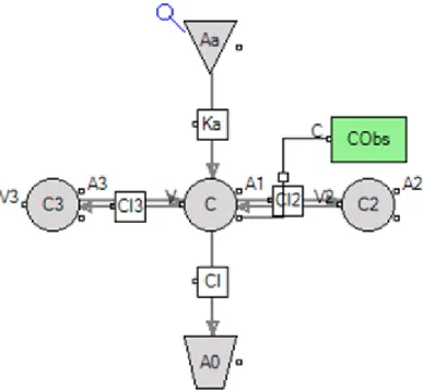
Figure 1.1: A three-compartment pharmacokinetic model
for each compartment.
dAa
dt =−Ka·Aa dA1
dt =Ka·Aa−Cl·C−Cl2·(C−C2)−Cl3·(C−C3) dA2
dt =Cl2·(C−C2) dA3
dt =Cl3·(C−C3)
where Aa is the amount in the absorption compartment, and A1, A2, and A3 are
the amounts in the central and peripheral compartments, respectively. The rate of absorption of the drug into the central compartment is denoted Ka. The flows of the
drug into and out of the peripheral compartments are denoted Cl2 and Cl3, and the
flow of drug out of the body is denotedCl. The corresponding volumes associated with
each compartments areV, V2, and V3, respectively. Then, we have the concentrations
C = A1
V C2 =
A2
V2
C3 =
A3
V3
The equation for C represents the model for the individual in the hierarchy of models. However, one needs to account for unexplained variability. (Note: The above example assumes the kinetics of drug transfer are first order. However, variations of such a model that employ non-linear kinetics can also be accommodated.)
The model for the residual error accounts for overall uncertainty in the concen-trations over time. It captures all variability not captured by the specified fixed and random effects. The errors may weighted so that measurements with higher variabil-ity are given less weight compared with measurements with smaller variabilvariabil-ity. For example, under a constant CV percentage error model,
CObs =C·(1 +C)
where CObs is the observed concentration, C is the predicted concentration, and C is
the residual error. C is almost always assumed to follow a univariate normal
distribu-tion with mean 0 and variance σ2. With a constant CV percent error model, higher
concentration measurements (which tend to be more variable) are given less weight (Gabrielsson and Weiner, 2000). Other options for weighting include
1. Additive (Uniform): CObs =C+C
2. Log-Additive (equivalent to fitting a model to the log of the observations): CObs =
ln(CObs) = ln(C) +C
3. Power: CObs = C+Cpower·C. Special case: Power=0.5 is Poisson weighting:
CObs =C+C0.5·C
4. Mixed is a combination of Proportional and Additive: CObs =C+C+C·C·
CM ixRatio
5. Custom
For a non-population model, the parameters Ka, V, Cl, V2, Cl2, V3, and Cl3 are
modeled with fixed effects only– that is, they are estimated separately for each indi-vidual. For a population model, one estimates the population mean values, and the amount each subject’s values deviate from the population means in a simultaneous fit of all subject’s data. In a population model, the PK parameters can be modeled with regression equations containing fixed effects, covariates, and random effects. The equa-tions for the PK parameters represent the model for the population in the hierarchy of models. For example,
Ka =θKa ·exp(ηKa+ηKa,P1P1+ηKa,P2P2)
V = (θV +dV dT rt·T rt)·exp(ηV)
V2 = (θV2 +dV2dF ed·F ed)·exp(ηV2)
V3 = (θV3 + (W/W t¯ )
dV3dW t)·exp(η
V3)
Cl = (θCl+dCldGene·Gene)·exp(ηCl)
Cl2 =θCl2 ·exp(ηCl2)
Cl3 =θCl3 ·exp(ηCl3)
whereθx denotes the fixed effect or typical value of a PK parameter x, andηx denotes
a random effect for a PK parameterx. The distribution of PK parameters is generally skewed to the right, and is often model with a log-normal distribution (this is why the
random effects are often exponentiated in the equations for the PK parameters). The vector of random effects is assumed to follow a multivariate normal distribution with mean 0 and variance-covariance matrix Ω. Ω may be diagonal, full block, or block diagonal.
Covariates such asT rt, an indicator that a specific drug was given, can be included. In the example above, F ed and Geneare indicators that a subject was fed and that a certain gene is present, andW tis a continuous variable for the body weight of a subject. ( ¯W t represents the mean of W t across all subjects.) The effects of the covariates on the PK parameters are given by dV dT rt,dV2dF ed, dV3dW t, and dCldGene.
Occasion covariates such as P1, an indicator for the first set of visits, and P2, an
indicator for the second set of visits, are typically included with random effects such as
ηKa,P1 and ηKa,P2. They are usually assumed to be independent, normally distributed
with mean 0 and equal variance.
Hence, population pharmacokinetic models are non-linear mixed effects models. The differential equations may or may not have a closed-form solution, and are solved either analytically or numerically. The parameters are estimated using one of the various algorithms available such as first order conditional estimation with interaction (FOCEI) (Bonate, 2006).
1.2.3
Population PK/PD Modeling Procedure
Exploratory Analysis
The exploratory analysis consists of plotting and summarizing the data in a tab-ular format. Individual modeling of concentration data, via compartmental modeling or non-compartmental analysis, may be performed to obtain initial estimates for the population model. Linear regression of the natural log of the PK parameters to the covariates of interest may be done as part of the exploratory analysis. Linear regression may also be used to determine the structure of the PK model (for example, if clear-ance changes with dose, one may consider a Michaelis-Menten model for clearclear-ance) (Gabrielsson and Weiner, 2000).
A Michaelis-Menten model for clearance may have the form Cl = (Vmax/(Km + C)) where Vmax (maximum metabolic rate) and Km (Michaelis Menten constant) are parameters, and C is the predicted concentration. Drugs such as Ethanol exhibit Michaelis-Menten pharmacokinetics. From inspection of the equation for clearance, one can see that the Michaelis-Menten clearance decreases as the concentration increases. This can happen when the metabolizing enzymes become saturated, making the process of metabolism slower with an increase in drug concentration (Gabrielsson and Weiner, 2000).
Population Model Development
Model development consists of spelling out objectives, hypotheses, and assumptions, followed by model building (FDA, 1999). The proposed model building procedure will depend on the objectives, hypotheses, and assumptions. For example, if whether or not a subject is fed is expected to have an effect on the PK, one will plan to include a covariate for fed/fasted state prior to doing the model building and plan to test the hypothesis that fed/fasted state has no effect on the PK during the model building
process.
Population Model Building
Model building consists of three steps: Base/Structural Model, Covariate Model, and Covariance Model (FDA, 1999).
Base/Structural Model
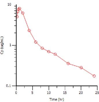
The structure of the PK model is determined largely during the exploratory analysis, where the concentrations are plotted on the log scale versus time. The number of compartments may be determined by observing the number of distinct phases visible in the plot (Gabrielsson and Weiner, 2000). For example, Figure 1.2 is a plot of the drug concentration versus time for a drug that exhibits two compartment pharmacokinetics. In Figure 1.2, the concentration increases from zero as the drug is absorbed, until it reaches the maximum concentration,Cmax. After reachingCmax, the drug concentration
in plasma decreases sharply at first if the distribution is rapid, then decreases again at a different rate. The two distinct phases afterCmax are modeled with two compartments:
a central compartment and a peripheral compartment. However, the steeper decline may represent elimination if distribution is slower than elimination.
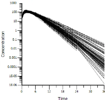
Imagine having several curves like Figure 1.2 in a single plot, varying slightly from one another, representing drug concentrations for several individuals (see Figure 2.5 for an example). In that case, the base/structural population PK model would be a two compartment model with random effects for the PK parameters Ka, V, Cl, V2, and
Cl2. A non-linear mixed effects model is generally used to predict average/population
Figure 1.2: Drug concentration versus time for a two-compartment model
individual deviates from the population PK value.
To obtain initial estimates for the fixed effects PK parameters in the base/structural model, one may use traditional methods such as curve stripping (Gibaldi and Perrier, 1975). This method is built in to the WinNonlin Classic models and is performed automatically when the defaults are accepted. One may also use non-compartmental analysis (Gibaldi and Perrier, 1975) for obtaining initial estimates. Also, the Naive Pooled method in Phoenix NLME (Pharsight) can be used to get rough estimates for the fixed effects (essentially FOCEI with random effects parameters frozen to 0), especially when the data are relatively sparse.
Once fixed effects initial estimates are found, one builds up to obtaining rough estimates for the variances and covariances of the random effects. A method called First Order (FO) can be used to accomplish this (Sheiner, Rosenberg and Melmon, 1972), as well as iterative two stage Expectation-Maximization (IT2S-EM) in Phoenix NLME (Ette and Williams, 2004).
Estimation Methods
The covariate selection, covariance structure selection, and final model are fitted with an FOCEI method, QRPEM, or a Laplacian method. Two kinds of FOCEI, First Order Conditional Estimation- Extended Least Squares (FOCE-ELS) and First Order Conditional Estimation Lindstrom-Bates (FOCE L-B), are implemented in Phoenix NLME. Of the FOCEI methods, the Lindstrom Bates method tends to run faster than the ELS method. The Laplacian method is considered to be the most numerically correct of all the methods, and can be used for things like Poisson regression or other regression models where the likelihood function is specified by the user, though it generally takes longer to run. See (Ette and Williams, 2004) for a description of these methods. QRPEM was recently implemented in Phoenix NLME (in March of 2012) and has been excellent at fitting the more complex models for this work (Leary and Dunlavey, 2012).
Covariate Model
is determined.
Covariance Model
The inter-subject covariance model is defined by the structure of the Ω matrix. Ran-dom effects with low shrinkages (less than around 0.3) are kept in the model (Karlsson and Savic, 2007) (Savic and Karlsson, 2007), otherwise, random effects may be removed. For the random effects that are kept, the Ω matrix may be full block (all random effects correlated), block diagonal (some random effects correlated, some independent of the others), or diagonal (no random effects correlated). A scatter plot of the etas versus the etas for the final covariate model may be used to help determine the structure of Ω.
To obtain a robust estimate of the Ω matrix, one may use a non-parametric method. One is built in to Phoenix NLME. It starts with a parametric solution, then performs parametric iteration(s). If the estimate of the Ω matrix found using the non-parametric method is vastly different from that of the non-parametric method, it may indicate that one or more of the random effects has a bimodal distribution or some other deviation from a normal distribution. This may mean that a covariate was left out that should have been included (Davidian and Giltinan, 1995).
Model Validation
Once a final model is determined, model validation is done. Model validation may be performed using bootstrapping or predictive check. Consider a dataset containing concentration-time data for n subjects. Suppose one were to take a simple random sample with replacement of size n, fit a model, and obtain estimates. Then, perform
thisxtimes, and summarize the model estimates across the xsamples. This procedure is known as bootstrapping (Efron and Tibshirani, 1986) for population PK. Histograms of the bootstrapped model estimates may also be generated. It is known that the estimates of the standard errors of the model estimates can be biased. To account for this, boot-strapping is often employed to get better estimates of the variability. In many cases, it is the only way to obtain estimates of the variability of the model estimates, because the standard errors cannot always be calculated via matrix decomposition (Yafune and Ishiguro, 1999).
Predictive check is used to generate a population of subjects based on the fitted model, and then visually determine if this distribution provides good coverage of the underlying data on which the model was based (Karlsson and Holford, 2008). Beginning with a final model, the final model estimates are assumed to be correct. Then, based on the model assumptions that C is normally distributed with mean 0 and variance
σ2, and η follows a multivariate normal distribution with mean 0 and variance Ω, new
concentration-time observations are simulated for x replicates of n subjects. If the measurements are not taken at the same times for all subjects, similar times are binned (using an algorithm such as the k-means clustering algorithm). For each time bin, quantiles of the observed and simulated concentrations are calculated. A visual plot of the observed data with bands for the observed and simulated quantiles is used to determine whether the model fits the data.
1.2.4
Challenges in Population PK/PD Modeling
resulting in having to set some parameters to a constant (or zero) or fitting a less complex model. Covariate model building can be time consuming and lead to inflated type I error rates (Wahlby, Jonsson and Karlsson, 2001). Estimates of precision of parameters are often biased and require bootstrapping or other techniques. Depending on model complexity, richness of data and other issues, it may take hours (or days) to achieve convergence. Message Passing Interface (MPI) may be used to take advantage of multiple processors on a single machine in Phoenix NLME. Also, a grid or cluster of multiple computers may be used for parallel processing.
1.2.5
Smoothing Splines
A discussion of smoothing splines is given here because in Chapter 4 we will compare population PK models to smoothing splines for prediction of concentrations. Suppose we are given a set of response variables{yi}ni=1 and predictor variables {xi}ni=1 and we
wish to estimate eachyi based on f(xi), where f is a function that minimizes n
X
i=1
[yi−f(xi)]
2
+λ
Z
{f00(t)}2dt (1.1) Any suchfmust be an element of the Sobolev space of functions with second derivatives that are square integrable. The tuning parameter λ controls the tradeoff between goodness of fit and smoothness. When λ = ∞, no second derivative is allowed for f, meaning that f must be linear and (4.2) reduces to the ordinary least squares criteria. When λ= 0, then any f that interpolates the data will minimize (4.2).
It can be shown that (4.2) is minimized when f is a natural cubic spline with knots at eachxi (Hastie, Tibshirani and Friedman, 2008). Letx(1), x(2), . . . , x(n) be the order
statistics of thexi’s. Then a natural cubic splinef(x) with knots x1, x2, . . . , xnsatisfies
the following properties:
1. f(x) is a a piecewise cubic polynomial. In particular, f(x) is a cubic polynomial on [x(1), x(2)],[x(2), x(3)], . . . ,[x(n−1), x(n)].
2. f(x) and its first two derivatives are continuous on [x(1), x(n)].
3. f(j)(x
(1)) = f(j)(x(n)) = 0 for j = 2,3. In other words, the second and third
derivatives of f are zero at the boundary knots, which implies that f is linear outside the boundary knots.
See (Welham, 2009) or (Dierckx, 1995). For a complete description of smoothing splines and methods for fitting spline models (including the choice of the tuning parameterλ), see (Hastie, Tibshirani and Friedman, 2008).
1.2.6
Cross-Validation
A discussion of cross-validation is given here because in Chapters 2 and 3 we propose new cross-validation methods for population PK/PD covariate model building. Cross-validation is a method for evaluating the expected accuracy of a predictive model. Suppose we have a response variable Y and a predictor variable X and we seek to estimateY based onX. Using the observedX’s andY’s we may estimate a function ˆf
such that our estimated value ofY (which we call ˆY) is equal to ˆf(X). Cross-validation is an estimate of the expected loss function for estimatingY based on ˆf(X). If we use squared error loss (as is conventional in population PK modeling), then cross-validation is an estimate ofE
Y −fˆ(X)2
.
A brief explanation of cross-validation is as follows: First, the data is divided into
K partitions of roughly equal size. For the kth partition, a model is fit to predict Y
estimates of prediction error are combined. Formally, let ˆf−k be the estimated value of
f when the kth partition is removed, and suppose the indices of the observations in the
kth partition are contained in Kk. Then the cross-validation estimate of the expected
prediction error is equal to
1 n k X i=1 X
j∈Ki
yj −fˆ−i(xj)
2
Heren denotes the number of observations in the data set. For a more detailed discus-sion of cross-validation, see (Hastie, Tibshirani and Friedman, 2008).
1.2.7
Current Uses of Cross-Validation in Population PK/PD
As mentioned earlier, covariate model building may be carried out using likelihood ratio tests (LRTs) when candidate models are nested. However, there may be an inflated type I error rate associated with the LRTs (Bertrand et al., 2009). For model comparison, cross validation has been unsuccessful at finding covariate effects when other methods seem to imply that covariate effects exist (Zomorodi et al., 1998), (Fiset et al., 1995). However, cross validation has been successful at identifying models with major structural differences (Valodia et al., 2000).
Cross validation is not often done with population PK modeling (Brendel et al., 2007). In one case (Bailey, Mora and Shafer, 1996), data was pooled across subjects to fit a model as though the data were obtained from a single subject. Subjects were removed, one at a time, and the accuracy of the predicted observations with subsets of the data was assessed. The method we propose is different because it does not pool the data across subjects prior to modeling, and we use it to compare candidate mod-els rather than to assess accuracy of prediction. Another paper (Hooker et al., 2008) describes removing a subject at a time to estimate model parameters, then predicting
PK parameters using the covariate values for the subject that was removed and com-paring those with the PK parameters obtained using the full data set, to evaluate the final model and identify influential individuals. The method we propose is different in that it uses a post-hoc step to calculate random effect values for the subject that is removed, and instead of evaluating a final model or identifying influential individuals we use cross validation to compare candidate models.
One article, (Ralph et al., 2006) calculates a prediction error for each subject in the model parameters, and a paired t-test is done on the prediction error between a base and full model to assess whether difference in imprecision of clearance between models is significant. The prediction error is calculated as the difference in the individual and population estimate divided by the individual estimate, times 100 percent, where the individual estimate is obtained using cross validation. The full model is only found to be correct with high levels of the covariate. This is fairly similar to the method we propose, except the statistic is different and a t-test is not employed, thus making it easier to find a covariate effect if there is one.
In (Zomorodi et al., 1998), cross validation is performed and weighted residuals for subjects left out are used to compare a base and full model. Predictions obtained for subjects left out may or may not have been based on the post hoc parameter estimates (article not clear). The base model is found to be better with the cross validation approach, but in other parts of paper the covariate is found to be significant. Actual model development was performed using a likelihood based approach. Later in this work, we explain why covariate effects go unidentified when the cross validation prediction error in the y’s is used for comparing models in the population PK/PD setting.
Predictive performance of the final model is assessed using cross validation. In (Ker-busch et al., 2001), “if model predictions based on partial dataset were in accordance with predictions of full dataset, predictive ability of model was confirmed” (here authors cited (Efron and Tibshirani, 1993)).
Covariate models are compared using cross validation in (Fiset et al., 1995). Cross validation error in concentrations ((Obs - Pred)/Pred)*100 was used for comparing covariate models. All models in the comparison had similar cross validation results. Actual model development was performed using likelihood based approaches.
A poster presented in 2001 at PAGE by Ribbing (Ribbing and Jonsson, 2001) pro-poses a method for cross validation, referred to as cross model validation (CMV). With this method, cross validation is used with the objective function value (similar to log likelihood function) to select a covariate model. A similar method is proposed in (Kat-sube et al., 2011).
It may be that researchers were finding that cross validation as it is typically done for population PK/PD modeling is not helpful for detecting covariates. In (Wahlby, Jonsson and Karlsson, 2001), for the cross validation, one concentration data point for each parameter, the point at which the parameter is most sensitive, was chosen based on partial derivatives. In the cross-validation, the models showed similar predictive ability with respect to both measures of the concentration prediction errors defined in the article. It seems that even using the cross validation prediction error in the y’s at the points that are most sensitive to the PK parameter with the covariate of interest does not help to elucidate a covariate relationship when one appears to exist.
It will be shown in Chapter 2 that when covariate effects are present in an underlying population PK/PD model, a misspecification of failing to include a covariate effect may not hurt the overall predictive performance of the model in the outcome variable or concentration. Random effects in the pharmacokinetic parameters can make up for
the lack of the covariate. Therefore, cross validation metrics that involve the predicted concentration errors will fail to identify a covariate effect. We instead propose using the post hoc estimates of the random effects as metrics for identifying covariate effects in population PK/PD models.
1.2.8
Automated Covariate Selection in Population PK/PD
A commonly used method for automated covariate selection in population PK/PD modeling is forward addition then backward elimination. It is often referred to as “stepwise”, though it’s different from the stepwise procedure used in traditional linear regression in that it does forward once, then backward once (Jonsson and Karlsson, 1998). Another method is GAM (Mandema, Verotta and Sheiner, 1992). A comparison of these methods can be found in (Wahlby, Jonsson and Karlsson, 2002). Maitre first proposed looking at the plots of the random effects versus the covariates to aid covariate model selection (Maitre et al., 1991). It was found that tree based modeling with cross validation to determine the tree size can help identify possible covariate models (Jonsson and Karlsson, 1999), but it does not seem that the cross validation method described involved re-fitting of the population model. This paper further explores the use of cross validation for automated covariate selection, with cross validation in the post hoc etas obtained from re-fitting population models.
1.3
Proposed Research
Chapter 2
Cross validation for Longitudinal
Mixed Effects Models
2.1
Overview
2.2
Introduction
Cross validation has been used in various forms in the population pharmacokinetic setting. With all the variations, there are two common uses of cross validation currently being used for population PK/PD modeling. Those are final model validation and model comparison.
For model comparison, cross validation has been unsuccessful at finding covariate effects when other methods seem to imply that covariate effects exist (Zomorodi et al., 1998), (Fiset et al., 1995). However, cross validation has been successful at identifying models with major structural differences (Valodia et al., 2000). In these instances, cross validation error in the y’s was used for model comparison. There are other methods available to compare population pharmacokinetic/pharmacodynamic (PK/PD) models, such as the likelihood ratio test (LRT), however there may be an inflated Type I error rate associated with these methods in the population PK/PD setting (Bertrand et al., 2009).
When covariate effects are present in an underlying population PK/PD model, a misspecification of failing to include a covariate effect may not hurt the overall predictive performance of the model in the outcome variable y or concentration. Random effects in the pharmacokinetic parameters can make up for the lack of the covariate. Therefore, cross validation metrics that involve the predicted outcome or concentration errors (y’s) will often fail to identify a covariate effect.
Population pharmacokinetic and pharmacodynamic (PK/PD) modeling is the char-acterization of the distribution of probable PK/PD outcomes (parameters, concentra-tions, responses, etc.) in a population of interest. These models consist of fixed and random effects. The fixed effects describe the relationship between explanatory vari-ables such as age, body weight, gender, and pharmacokinetic outcomes. The random effects quantify unexplained variation in PK/PD outcomes.
Population PK models are hierarchical. There is a model for the individual, a model for the population, and a model for the residual error. The individual model consists of the curve of drug concentrations over time, a compartmental model. The pharmacokinetic compartmental model is similar to a black box engineering model. Each of the compartments is like a black box, where a system of differential equations is derived based on the law of conservation of mass (Sandler, 1999).
The equations for the PK parameters represent the model for the population in the hierarchy of models. The PK parameters are modeled with regression equations containing fixed effects, covariates, and random effects (etas). The vector of random effects (eta) is assumed to follow a multivariate normal distribution with mean 0 and variance-covariance matrix Ω. Ω may be diagonal, full block, or block diagonal.
The model for the residual error accounts for overall uncertainty in the concentra-tions over time. The errors may weighted so that measurements with higher variability are given less weight compared with measurements with smaller variability.
Hence, population pharmacokinetic models are non-linear mixed effects models. The differential equations may or may not have a closed-form solution, and are solved either analytically or numerically. The parameters are estimated using one of the various algorithms available such as first order conditional estimation with interaction (FOCEI). See (Wang, 2007) for a mathematical description of these algorithms.
Once model parameters are estimated using an algorithm such as FOCEI, one may
fix the values of the model estimates and perform a post-hoc calculation to obtain random effect values (etas) for each subject. Thus, one may fit a model to a subset of the data and obtain random effect values for the full data set.
2.2.1
Cross-Validation
Cross-validation is a method for evaluating the expected accuracy of a predictive model. Suppose we have a response variable Y and a predictor variable X and we seek to estimate Y based on X. Using the observed X’s and Y’s we may estimate a function ˆf such that our estimated value of Y (which we call ˆY) is equal to ˆf(X). Cross-validation is an estimate of the expected loss function for estimating Y based on ˆf(X). If we use squared error loss (as is conventional in population PK modeling), then cross-validation is an estimate of E
Y −fˆ(X) 2
.
A brief explanation of cross-validation is as follows: First, the data is divided into
K partitions of roughly equal size. For the kth partition, a model is fit to predict Y
based on X using the K−1 other partitions of the data. (Note that the kth partition is not used to fit the model.) Then the model is used to predict Y based on X for the data in the kth partition. This process is repeated for k = 1,2. . . , K, and the K
estimates of prediction error are combined. Formally, let ˆf−k be the estimated value of
f when the kth partition is removed, and suppose the indices of the observations in the
kth partition are contained in Kk. Then the cross-validation estimate of the expected
prediction error is equal to
1 n k X i=1 X
j∈Ki
yj −fˆ−i(xj)
2
Cross validation is not often done with population PK modeling (Brendel et al., 2007). In one case (Bailey, Mora and Shafer, 1996), data was pooled across subjects to fit a model as though the data were obtained from a single subject. Subjects were removed, one at a time, and the accuracy of the predicted observations with subsets of the data was assessed. The method we propose is different because it does not pool the data across subjects prior to modeling, and we use it to compare candidate mod-els rather than to assess accuracy of prediction. Another paper (Hooker et al., 2008) describes removing a subject at a time to estimate model parameters, then predicting PK parameters using the covariate values for the subject that was removed and com-paring those with the PK parameters obtained using the full data set, to evaluate the final model and identify influential individuals. The method we propose is different in that it uses a post-hoc step to calculate random effect values for the subject that is removed, and instead of evaluating a final model or identifying influential individuals we use cross validation to compare candidate models.
2.3
Methods
2.3.1
Comparing models with major structural differences
In this case, a researcher may want to compare models with different numbers of compartments, such as a one-compartment model with a two-compartment model. This method is designed to detect differences in models that affect the overall shape of the curve.
Consider a dataset with subjects i, i = 1, ..., n. Each subject has observations yij
forj = 1, ...,ti (tibeing the number of time points or discrete values of the independent
variable for which there are observations for subject i). The statistic can be calculated as follows.
For i= 1 to n:
1. Remove subject i from the dataset
2. Fit a mixed effects model to the subset of the data
3. Accept all parameter estimates from the last run, and freeze the parameters to those values
4. Fit the same model to the whole dataset, without any major iterations, estimat-ing only the post hoc values of the random effects (Phoenix NLME: NITER=0. NONMEM: MAXITER=0, POSTHOC=Y)
5. Calculate predicted values for subject i (the subject that was left out)
6. Take the average of the squared individual residuals for the subject that was left out (over all time points or over all values of the independent variable ti)
Take the average of the quantity in step 6 over all subjects.
This sequence of steps can also be represented by the equation
mP RESS = 1
n
n
X
i=1
ti
P
j=1
(yij−yˆij,−i)2
ti (2.1)
whereyij is the observed value for theith subject at the jth time point or
indepen-dent variable value. ˆyij,−i is the predicted value for theith subject at thejth time point
For purposes of exploration, another statistic that takes into account the weighting can be calculated
wtmP RESS = 1
n n X i=1 ti P j=1
W T IRES2
ij,−i
ti , W T IRESij,−i =
√
wtij,−i(yij −yˆij,−i)
ˆ
σ−i
(2.2)
where W T IRESij,−i is the individual weighted residual for subject i at time or
independent variable value j in a model where subject i is left out and post hocs are obtained, and wtij,−i is the weight defined by the residual error model (equal to the
squared reciprocal of ˆyij,−i for constant CV error models or 1 for additive error models),
and ˆσ−2i is the estimated residual variance.
When comparing models, the following steps should be applied. If the model with less parameters has a value of the statistic less than or equal to that of the model with more parameters, the model with less parameters should be chosen. For cases where the statistic for the model with more parameters is smaller than that of the model with less parameters, and furthermore, if the statistic for the model with less parameters is within one standard error of the statistic of the model with more parameters, the model with the smaller number of parameters should be chosen. Otherwise, if the model with more parameters has a value of the statistic that is more than one standard error below that of the model with less parameters, the model with more parameters should be chosen. The standard error employed should be that of the model with the smallest value of the statistic.
Alternatively, one may follow the same procedure, removing more than one subject at a time. For example, remove 10 percent of subjects at a time, fit a model, obtain predictions for the subjects left out including the post hoc values of the parameters. Square the individual residuals, average those over the independent variable for each
subject, average over subjects.
This method is similar to, or possibly the same as, cross validation methods already established, though it’s not clear whether current methods include calculating the post hoc parameter values to obtain predictions for the subjects that are left out.
2.3.2
Comparing covariate models
In this case, a researcher may want to compare models with and without covariate effects, such as a model with an age effect on clearance versus a model without an age effect on clearance. This method is designed to detect differences in models that affect the equations for the parameters.
Consider a dataset with subjectsi,i= 1, ...,n. Each subject has observationsyij for
j = 1, ..., ti (ti being the number of time points or discrete values of the independent
variable for which there are observations for subject i). The question of interest is whether or not a fixed effect dPdV for a covariate V should be included in an equation for a parameter P, having fixed effect tvP and random effect ηP. The equation for P
could have any of the typical forms used in population PK/PD modeling, for example,
P =tvP ·(V /mean(V))dP dV ·exp(ηP) (2.3)
and one wishes to compare it with a model having no covariate effect
P =tvP ·exp(ηP) (2.4)
If a covariate, V, has an effect on a parameter, P, the unexplained error in P, modeled by
ηP, when V is left out of the model tends to have higher variance. By including covariate
V in the model, we wish to reduce the unexplained error in P, which is represented by
is needed. While the distribution of ηP under the null and alternative hypotheses is
unknown, cross validation can be performed. We propose a statistic for determining whether a covariate, V, is needed for explaining variability in a parameter, P, when P is modeled with a random effect “eta”,ηP.
The statistic can be calculated as follows.
For i= 1 to n:
1. Remove subject i from the dataset
2. Fit a mixed effects model to the subset of the data
3. Accept all parameter estimates from the last run, and freeze the parameters to those values
4. Fit the same model to the whole dataset, without any major iterations, estimat-ing only the post hoc values of the random effects (Phoenix NLME: NITER=0. NONMEM: MAXITER=0, POSTHOC=Y)
5. Square the post hoc eta estimate for the subject that was left out for the parameter of interest
Take the average of the quantity in step 5 over all subjects.
This sequence of steps can also be represented by the equation
nP RESS = 1
n
n
X
i=1
(ˆηPi,−i)
2 (2.5)
Where ˆηPi,−i is the post hoc “eta” estimate for the ith subject for parameter P in
When comparing models, the following steps should be applied. If the model with less parameters has a value of the statistic less than or equal to that of the model with more parameters, the model with less parameters should be chosen. For cases where the statistic for the model with more parameters is smaller than that of the model with less parameters, and furthermore, if the statistic for the model with less parameters is within one standard error of the statistic of the model with more parameters, the model with the smaller number of parameters should be chosen. Otherwise, if the model with more parameters has a value of the statistic that is more than one standard error below that of the model with less parameters, the model with more parameters should be chosen. The standard error employed should be that of the model with the smallest value of the statistic.
Alternatively, one may follow the same procedure, removing more than one subject at a time. For example, remove 10 percent of subjects at a time, fit a model, calculate the post hoc values for the subjects left out, square the post hoc etas, average them over subjects.
2.4
Simulation Example 1
A one-compartment, extravascular model was simulated with eight subjects using Pharsight’s Trial Simulator. The equations for the model are as follows.
dAa
dt =−Ka·Aa dA1
dt =Ka·Aa−Cl·C C = A1
A 10 percent constant CV percentage was simulated for the residual error. CObs = C * (1 + CEps) where Var(CEps) = 0.01
A fixed effect was added to the absorption rate parameter, Ka. All other parameters were simulated with fixed and random effects.
Ka =tvKa
V =tvV ·exp(nV)
Cl =tvCl·exp(nCl)
The fixed effects for the PK parameters were assumed to be normally distributed at the study level (varying across replicates) with means listed below and standard deviations of 0.1.
mean(tvKa) = 0.35
mean(tvV) = 13.5
mean(tvCl) = 7.4
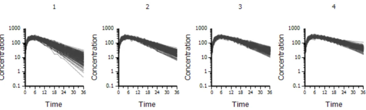
The random effects (nV and nCl) were simulated to be independent and normally distributed at the subject level (varying across subjects) with means of 0 and variances of 0.01. A covariate, GENDER, was simulated, so that there were 50 percent males and 50 percent females. A covariate, BODYWEIGHT, was simulated with a mean of 70 kg for males, 65 kg for females and a standard deviation of 15 for both groups. A covariate, Age, was simulated, with a mean of 40 years and a standard deviation of 10. None of the covariates were simulated to have any effect on the parameters. The true underlying model had no covariate effects. A dose of 5617 was administered at time 0, as an extravascular dose. Two hundred replicates were simulated. See Figure 2.1 for a plot of the simulated data.
The base model was a one compartment extravascular model with random effects for V and Cl and no age effect on clearance. The full model was a one compartment
Figure 2.1: Simulation Example 1 data
extravascular model with random effects for V and Cl and an age effect on clearance. Base (correct) model
Ka =tvKa
V =tvV ·exp(nV)
Cl =tvCl·exp(nCl) Full (incorrect) model
Ka =tvKa
V =tvV ·exp(nV)
Cl =tvCl·(Age/40)dCldAge·exp(nCl)
were all 0.1, close to the true value of 0.01.
2.5
Simulation Example 2
A one-compartment, extravascular model was simulated with eight subjects using Pharsight’s Trial Simulator. The equations for the model are as follows.
dAa
dt =−Ka·Aa dA1
dt =Ka·Aa−Cl·C C = A1
V
A 10 percent constant CV percentage was simulated for the residual error. CObs = C * (1 + CEps) where Var(CEps) = 0.01
A fixed effect was added to the absorption rate parameter, Ka. All other parameters were simulated with fixed and random effects. The systemic clearance was simulated with an age effect.
Ka =tvKa
V =tvV ·exp(nV)
Cl =tvCl·(Age/40)dCldAge·exp(nCl)
The fixed effects (tvKa, tvV, tvCl, and dCldAge) were assumed to be normally distributed at the study level (varying across replicates) with means listed below and
standard deviations of 0.05, 0.1, 0.05, and 0.04, respectively.
mean(tvKa) = 0.35
mean(tvV) = 13.5
mean(tvCl) = 1.2
mean(dCldAge) = −0.9
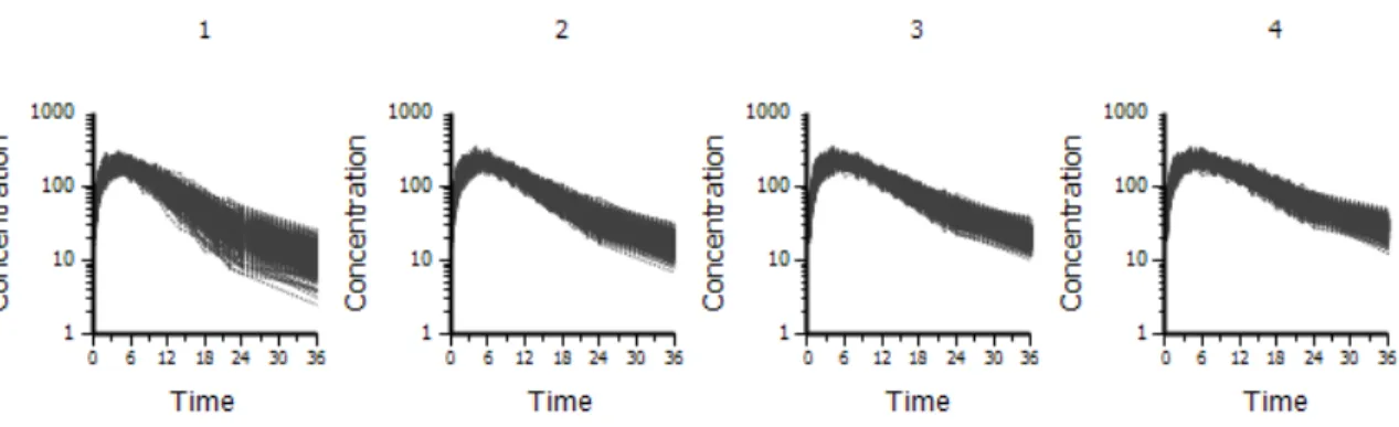
The random effects (nV and nCl) were simulated to be independent and normally distributed at the subject level (varying across subjects) with means of 0 and variances of 0.01. A covariate, GENDER, was simulated, so that there were 50 percent males and 50 percent females. A covariate, BODYWEIGHT, was simulated with a mean of 70 kg for males, 65 kg for females and a standard deviation of 15 for both groups. A covariate, Age, was simulated, with a mean of 40 years and a standard deviation of 10. The true underlying model had a covariate effect– an age effect on clearance. A dose of 5617 was administered at time 0, as an extravascular dose. Two hundred replicates were simulated. See Figure 2.2 for a plot of the simulated data, with clearance decreasing with age.
Figure 2.2: Simulation Example 2 data, by age quartiles
Base (incorrect) model
Ka =tvKa
V =tvV ·exp(nV)
Cl =tvCl·exp(nCl) Full (correct) model
Ka =tvKa
V =tvV ·exp(nV)
Cl =tvCl·(Age/40)dCldAge·exp(nCl)
Where tvKa, tvV, tvCl, and dCldAge are fixed effects parameters to be estimated. Initial estimates for the fixed effects parameters (tvKa, tvV, tvCl, and dCldAge) were set to the true (simulated) parameter values. The initial estimates of the variances of the random effects were all 0.1, close to the true values of 0.01.
2.6
Simulation Example 3
A two-compartment, extravascular model was simulated with eight subjects using Pharsight’s Trial Simulator. The equations for the model are as follows.
dAa
dt =−Ka·Aa dA1
dt =Ka·Aa−Cl·C−Cl2·(C−C2) dA2
dt =Cl2·(C−C2) C = A1
V C2 = A2
V2
A 10 percent constant CV percentage was simulated for the residual error. CObs = C * (1 + CEps) where Var(CEps) = 0.01
A fixed effect was added to the absorption rate parameter, Ka. All other parameters were simulated with fixed and random effects. The systemic clearance was simulated with an age effect.
Ka =tvKa
V =tvV ·exp(nV)
V2 = tvV2·exp(nV2)
Cl =tvCl·(Age/40)dCldAge·exp(nCl)
Cl2 = tvCl2·exp(nCl2)
below and standard deviations of 0.05, 0.1, 0.1, 0.05, 0.05, and 0.04, respectively.
mean(tvKa) = 0.35
mean(tvV) = 13.5
mean(tvV2) = 36
mean(tvCl) = 1.2
mean(tvCl2) = 0.62
mean(dCldAge) = −0.9
The random effects (nV, nV2, nCl, and nCl2) were simulated to be independent and normally distributed at the subject level (varying across subjects) with means of 0 and variances of 0.01. A covariate, GENDER, was simulated, so that there were 50 percent males and 50 percent females. A covariate, BODYWEIGHT, was simulated with a mean of 70 kg for males, 65 kg for females and a standard deviation of 15 for both groups. A covariate, Age, was simulated, with a mean of 40 years and a standard deviation of 10. The true underlying model had a covariate effect– an age effect on clearance. A dose of 5617 was administered at time 0, as an extravascular dose. Two hundred replicates were simulated. See Figure 2.3 for a plot of the simulated data, with clearance decreasing with age.
Figure 2.3: Simulation Example 3 data, by age quartiles
The base model was a two compartment extravascular model with random effects
on V, V2, Cl, and Cl2 and no age effect on clearance. The full model was similar to the base model, but with an age effect included for Cl.
Base (incorrect) model
Ka =tvKa
V =tvV ·exp(nV)
V2 =tvV2·exp(nV2)
Cl =tvCl·exp(nCl)
Cl2 =tvCl2·exp(nCl2) Full (correct) model
Ka =tvKa
V =tvV ·exp(nV)
V2 = tvV2·exp(nV2)
Cl =tvCl·(Age/40)dCldAge·exp(nCl)
Cl2 = tvCl2·exp(nCl2)
Where tvKa, tvV, tvV2, tvCl, tvCl2, and dCldAge are fixed effects parameters to be estimated. Initial estimates for the fixed effects parameters (tvKa, tvV, tvV2, tvCl, tvCl2, and dCldAge) were set to the true (simulated) parameter values. The initial estimates of the variances of the random effects were all 0.1, close to the true values of 0.01.
2.7
Simulation Example 4
dAa
dt =−Ka·Aa dA1
dt =Ka·Aa−Cl·C C = A1
V
A 10 percent constant CV percentage was simulated for the residual error. CObs = C * (1 + CEps) where Var(CEps) = 0.01
A fixed effect was added to the absorption rate parameter, Ka. All other parameters were simulated with fixed and random effects. The systemic volume was simulated with a body weight effect. The systemic clearance was simulated with body weight (BW), age (Age), gender (Gender), and hepatic impairment (HI) effects.
Ka =tvKa
V =tvV ·(BW/70)dV dBW ·exp(nV)
Cl =tvCl·(BW/70)dCldBW ·(Age/40)dCldAge·(1 +dCldG·Gender)
·(1 +dCldHI ·HI)·exp(nCl)
The fixed effects (tvKa, tvV, tvCl, dVdBW, dCldBW, dCldAge, dCldG, and dCldHI) were assumed to be normally distributed at the study level (varying across replicates) with means listed below and standard deviations of 0.05, 0.1, 0.05, 0.1, 0.1, 0.04, 0.05,
and 0.05 respectively.
mean(tvKa) = 0.35
mean(tvV) = 13.5
mean(tvCl) = 1.2
mean(dV dBW) = 1
mean(dCldBW) = 0.75
mean(dCldAge) =−0.9
mean(dCldG) = 0.1
mean(dCldHI) =−0.2
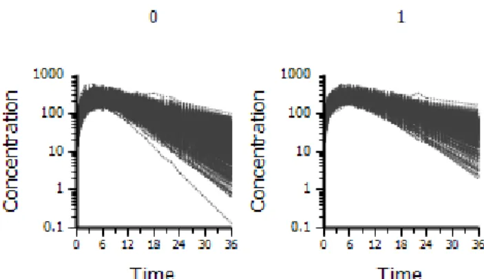
The random effects (nV and nCl) were simulated to be independent and normally distributed at the subject level (varying across subjects) with means of 0 and variances of 0.01. A covariate, Gender, was simulated, so that there were 50 percent males (Gender=1) and 50 percent females (Gender=0). A covariate for body weight, BW, was simulated with a mean of 70 kg for males, 65 kg for females and a standard deviation of 15 for both groups. A covariate, Age, was simulated, with a mean of 40 years and a standard deviation of 10. A covariate for hepatic impairment, “HI”, was simulated, with 70 percent not hepatically impaired (HI=0) and 30 percent hepatically impaired (HI=1). The true underlying model had five covariate effects– a body weight effect on volume, and age, body weight, gender, and hepatic impairment effects on clearance. A dose of 5617 was administered at time 0, as an extravascular dose. Two hundred replicates were simulated. See Figure 2.4 for a plot of the simulated data.
Figure 2.4: Simulation Example 4 data, by hepatic impairment
Base (incorrect) model
Ka =tvKa
V =tvV ·(BW/70)dV dBW ·exp(nV)
Cl =tvCl·(BW/70)dCldBW ·(Age/40)dCldAge·(1 +dCldG·Gender)·exp(nCl)
Full (correct) model
Ka =tvKa
V =tvV ·(BW/70)dV dBW ·exp(nV)
Cl =tvCl·(BW/70)dCldBW ·(Age/40)dCldAge·(1 +dCldG·Gender)
·(1 +dCldHI ·HI)·exp(nCl)
Where tvKa, tvV, tvCl, dVdBW, dCldBW, dCldAge, dCldG, and dCldHI are fixed effects parameters to be estimated. Initial estimates for the fixed effects parameters were set to the true (simulated) parameter values. The initial estimates of the variances of the random effects were all 0.1, close to the true values of 0.01.
2.8
Simulation Example 5
A two-compartment, extravascular model was simulated with six subjects using Pharsight’s Trial Simulator. The equations for the model are as follows.
dAa
dt =−Ka·Aa dA1
dt =Ka·Aa−Cl·C−Cl2·(C−C2) dA2
dt =Cl2·(C−C2) C = A1
V C2 = A2
V2
A 10 percent constant CV percentage was simulated for the residual error. CObs = C * (1 + CEps) where Var(CEps) = 0.01
A fixed effect was added to the absorption rate parameter, Ka. All other parameters were simulated with fixed and random effects.
Ka =tvKa
V =tvV ·exp(nV)
V2 =tvV2·exp(nV2)
Cl =tvCl·exp(nCl)
Cl2 =tvCl2·exp(nCl2)
standard deviation of 0.05 because when the absorption rate was smaller the portion of the curve for the first compartment became less pronounced in relation to the portion for the second compartment. Having a smaller standard deviation for Ka increased the chance that all the simulated profiles would have a characteristic two compartment shape.
mean(tvKa) = 0.35
mean(tvV) = 13.5
mean(tvV2) = 34
mean(tvCl) = 7.4
mean(tvCl2) = 1.2
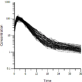
The random effects (nV, nV2, nCl, and nCl2) were simulated to be normally distributed at the subject level (varying across subjects) with means of 0 and variances of 0.01. A covariate, GENDER, was simulated, so that there were 50 percent males and 50 percent females. A covariate, BODYWEIGHT, was simulated with a mean of 70 kg for males, 65 kg for females and a standard deviation of 15 for both groups. A covariate, Age, was simulated, with a mean of 40 years and a standard deviation of 10. The true underlying model had no covariate effects. A dose of 5617 was administered at time 0, as an extravascular dose. One hundred replicates were simulated. See Figure 2.5 for a plot of the simulated data.
Pharsights Phoenix NLME was used to fit models to the simulated data. A base model with one compartment was fit to the simulated data. A full model with two compartments was fit.
Base (incorrect) model
Ka =tvKa
V =tvV ·exp(nV)
Figure 2.5: Simulation Example 5 data
Full (correct) model
Ka =tvKa
V =tvV ·exp(nV)
V2 =tvV2·exp(nV2)
Cl =tvCl·exp(nCl)
Cl2 =tvCl2·exp(nCl2)
Where tvKa, tvV, tvV2, tvCl, and tvCl2 are fixed effects parameters to be esti-mated. Initial estimates for the fixed effects parameters (tvKa, tvV, tvV2, tvCl, and tvCl2) were set to the true (simulated) parameter values. The initial estimates of the variances of the random effects were all 0.1, close to the true values of 0.01.
2.9
Computational details
different files, then to split replicate datasets into training datasets in separate folders. Each training dataset consisted of the full dataset for the given replicate except with concentrations and amounts set to missing for one subject. In each folder with each training dataset resided the full dataset for the corresponding replicate. One batch file was used to call another batch file to execute NLME in all the folders until all training datasets and all replicates were processed. First the batch files were called to run NLME with the training datasets to obtain model parameter estimates using the Lindstrom-Bates method (Lindstrom and Bates, 1990), then called to run NLME again in the same folder with the full datasets without any major iterations, starting from the last solution (!iflagrestart=1 in nlmeflags.asc), to obtain post hoc estimates for the subjects that had been removed.
This entire process was completed for a base model and a full model for each sim-ulation scenario.
2.10
Simulation Results
The results of the simulations are summarized in Tables 2.1, 2.2, 2.3, 2.4, and 2.5. If the true underlying model was the base model (as in the first scenario), a model comparison method was considered correct if it selected the base model. For AIC, BIC, and nPRESS, if the value for the base model was smaller than that of the full model, it was considered to be correct. For the mPRESS and wtmPRESS, the method was considered to be correct if the value of the statistic for the base model was less than the value of statistic for the full model. Otherwise, if the value of the statistic for the full model was smaller, it was still correct if the statistic for the base model was within one standard error of the statistic for the full model (employing the standard error of the statistic for the full model).
If the true underlying model was the full model, a model comparison method was
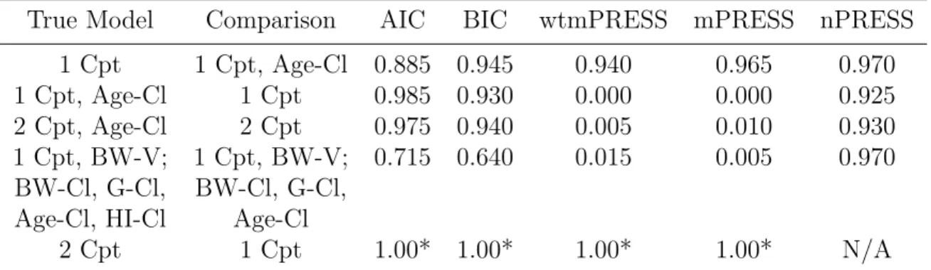
Table 2.1: Proportion correct out of 200 replicates
True Model Comparison AIC BIC wtmPRESS mPRESS nPRESS 1 Cpt 1 Cpt, Age-Cl 0.885 0.945 0.940 0.965 0.970 1 Cpt, Age-Cl 1 Cpt 0.985 0.930 0.000 0.000 0.925 2 Cpt, Age-Cl 2 Cpt 0.975 0.940 0.005 0.010 0.930 1 Cpt, BW-V; 1 Cpt, BW-V; 0.715 0.640 0.015 0.005 0.970 BW-Cl, G-Cl, BW-Cl, G-Cl,
Age-Cl, HI-Cl Age-Cl
2 Cpt 1 Cpt 1.00* 1.00* 1.00* 1.00* N/A
Cpt=Compartment, Age-Cl indicates age effect on clearance, BW=Body Weight, V=Volume, G=Gender, HI=Hepatic Impairment
*Based on 100 replicates
considered correct if it selected the full model. For AIC, BIC, and nPRESS, if the value was greater for the base model than for the full model, it was considered correct. For the mPRESS and wtmPRESS, the method was considered incorrect if the value of the statistic for the base model was smaller than the value of the statistic for the full model. Otherwise, if the value of the statistic for the base model was greater than the value of the statistic for the full model plus one standard error, it was considered to be correct (employing the standard error of the statistic for the full model).
model was one compartment with a body weight effect on volume, and body weight, gender, age, and hepatic impairment effects on clearance, nPRESS was correct in 97.0 percent of cases, whereas AIC and BIC were correct in 71.5 and 64.0 percent of cases, respectively.
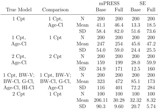
To emphasize the fact that the mPRESS and wtmPRESS statistics, which use the predicted values rather than the random effects for the parameters, should not be used for comparing different covariate models in the population PK/PD setting, mPRESS and wtmPRESS were calculated for all scenarios. They were wrong almost every time when the true model had a covariate effect. The predicted values are just as accurate with and without the covariate effect when the true model has a covariate effect, because the etas (e.g., nCl) will always compensate for a missing covariate in a parameter (e.g., Cl). This is why the nPRESS and not the mPRESS, nor the wtmPRESS, should be employed for situations when one wishes to compare different covariate models.
All four applicable methods (AIC, BIC, mPRESS, and wtmPRESS) correctly iden-tified the two compartment model with random effects on V, V2, Cl, and Cl2 as the correct model when the base model was a one compartment model with random effects on V and Cl in 100 out of 100 cases. This finding is of interest because the standard likelihood ratio test cannot be applied when there are random effects in the full model that aren’t present in the base model.
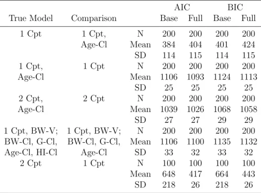
While AIC and BIC were not correct in all cases, the average AIC and BIC were smaller for the true underlying models when averaging across replicates.
For each replicate, the value of mPRESS, wtmPRESS, or nPRESS has a standard error associated with it. The standard error for each replicate is calculated as the sample standard error of mPRESS, wtmPRESS, or nPRESS divided by the square root of the number of subjects. The standard errors are summarized in Tables 2.3 and 2.4, along with the mean values of nPRESS, mPRESS, and wtmPRESS. The values
Table 2.2: Summary of AIC and BIC in simulation scenarios
AIC BIC
True Model Comparison Base Full Base Full
1 Cpt 1 Cpt, N 200 200 200 200
Age-Cl Mean 384 404 401 424 SD 114 115 114 115
1 Cpt, 1 Cpt N 200 200 200 200
Age-Cl Mean 1106 1093 1124 1113
SD 25 25 25 25
2 Cpt, 2 Cpt N 200 200 200 200
Age-Cl Mean 1039 1026 1068 1058
SD 27 27 29 29
1 Cpt, BW-V; 1 Cpt, BW-V; N 200 200 200 200 BW-Cl, G-Cl, BW-Cl, G-Cl, Mean 1106 1100 1135 1132
Age-Cl, HI-Cl Age-Cl SD 33 32 33 32
2 Cpt 1 Cpt N 100 100 100 100
Mean 648 417 664 443
SD 218 26 218 26
Table 2.3: Summary of nPRESS in simulations
nPRESS SE
True Model Comparison Base Full Base Full
1 Cpt 1 Cpt, N 200 200 200 200
Age-Cl Mean 0.136 0.919 0.022 0.403 SD 0.236 0.920 0.032 0.512
1 Cpt, 1 Cpt N 200 200 200 200
Age-Cl Mean 0.078 0.012 0.031 0.005
SD 0.056 0.010 0.022 0.005
2 Cpt, 2 Cpt N 200 200 200 200
Age-Cl Mean 0.144 0.024 0.077 0.020
SD 0.728 0.155 0.453 0.155 1 Cpt, BW-V; 1 Cpt, BW-V; N 200 200 200 200
BW-Cl, G-Cl, BW-Cl, G-Cl, Mean 1.700 0.124 0.626 0.081 Age-Cl, HI-Cl Age-Cl SD 2.577 0.281 2.515 0.214
Cpt=Compartment, Age-Cl indicates age effect on clearance, BW=Body Weight, V=Volume, G=Gender, HI=Hepatic Impairment
of nPRESS tended to be lower for the true underlying model in all scenarios. Because the eta will always compensate for a missing covariate, the mPRESS and wtmPRESS statistics should not be used for comparing covariate models, although they did perform well when the true underlying model had no covariate effect as well as for identifying the correct structural model.
2.11
Indomethacin Example
Pharsights Phoenix NLME was used to fit models to the published indomethacin dataset (Kwan et al., 1976). The indomethacin dataset, containing six subjects with eleven observations each, was fit using a two-compartment IV bolus model with Clear-ance parameterization and a proportional residual error model. Concentration units of ug/mL were assumed, and a dose of 25000 ug at 0 hours was assumed. Random effects were added to the PK parameters V, Cl, V2, and Cl2, in the form ThetaX*exp(nX),
Table 2.4: Summary of mPRESS in simulations
mPRESS SE
True Model Comparison Base Full Base Full
1 Cpt 1 Cpt, N 200 200 200 200
Age-Cl Mean 41.1 46.4 13.3 18.5 SD 58.4 82.0 51.6 73.6
1 Cpt, 1 Cpt N 200 200 200 200
Age-Cl Mean 247 254 45.6 47.2
SD 54.0 59.0 24.4 25.5
2 Cpt, 2 Cpt N 200 200 200 200
Age-Cl Mean 159 199 28.0 59.9
SD 34.9 171 12.5 160 1 Cpt, BW-V; 1 Cpt, BW-V; N 200 200 200 200 BW-Cl, G-Cl, BW-Cl, G-Cl, Mean 323 472 85.1 173 Age-Cl, HI-Cl Age-Cl SD 116 401 72.2 284
2 Cpt 1 Cpt N 100 100 100 100
Mean 206.11 30.28 32.32 8.32 SD 90.3 9.60 20.7 5.74
Table 2.5: Summary of wtmPRESS in simulations
wtmPRESS SE
True Model Comparison Base Full Base Full
1 Cpt 1 Cpt, N 200 200 200 200
Age-Cl Mean 1.14 1.20 0.157 0.176 SD 0.303 0.388 0.064 0.154
1 Cpt, 1 Cpt N 200 200 200 200
Age-Cl Mean 0.967 1.01 0.144 0.154
SD 0.133 0.130 0.120 0.111
2 Cpt, 2 Cpt N 200 200 200 200
Age-Cl Mean 1.0096 1550* 0.154 1550*
SD 0.0995 21700* 0.071 21700* 1 Cpt, BW-V; 1 Cpt, BW-V; N 200 200 200 200
BW-Cl, G-Cl, BW-Cl, G-Cl, Mean 1.25 2.78 0.305 1.56 Age-Cl, HI-Cl Age-Cl SD 0.485 11.6 0.432 11.3
2 Cpt 1 Cpt N 100 100 100 100
Mean 14.7 1.14 3.09 0.233 SD 10.1 0.143 2.86 0.130
Cpt=Compartment, Age-Cl indicates age effect on clearance, BW=Body Weight, V=Volume, G=Gender, HI=Hepatic Impairment
*One of the replicates (161) had an inflated value for wtmPRESS. One subject was significantly younger than the others, and the effect of age on clearance was estimated to be around -22 instead of the true value of -0.9 in the model where this subject was left out. Hence the younger subject had inflated residuals.