Euclid preparation. III. Galaxy cluster detection in the wide photometric survey, performance and algorithm selection

June 12, 2019

Euclid

preparation III. Galaxy cluster detection in the wide

photometric survey, performance and algorithm selection

Euclid Collaboration, R. Adam

, M. Vannier

, S. Maurogordato

, A. Biviano

, C. Adami

, B. Ascaso

,

F. Bellagamba

, C. Benoist

, A. Cappi

, A. D´ıaz-S´anchez

, F. Durret

, S. Farrens

, A.H. Gonzalez

, A. Iovino

,

R. Licitra

, M. Maturi

, S. Mei

, A. Merson

, E. Munari

, R. Pello

, M. Ricci

, P.F. Rocci

,

M. Roncarelli

, F. Sarron

, Y. Amoura

, S. Andreon

, N. Apostolakos

, M. Arnaud

, S. Bardelli

, J. Bartlett

,

C.M. Baugh

, S. Borgani

, M. Brodwin

, F. Castander

, G. Castignani

, O. Cucciati

, G. De Lucia

,

P. Dubath

, P. Fosalba

, C. Giocoli

, H. Hoekstra

, G. Mamon

, J.B. Melin

, L. Moscardini

,

S. Paltani

, M. Radovich

, B. Sartoris

, M. Schultheis

, M. Sereno

, J. Weller

, C. Burigana

,

C. S. Carvalho

, L. Corcione

, H. Kurki-Suonio

, P. B. Lilje

, G. Sirri

, R. Toledo-Moreo

, and G. Zamorani

(Affiliations can be found after the references)

Received June 12, 2019/Accepted –

Abstract

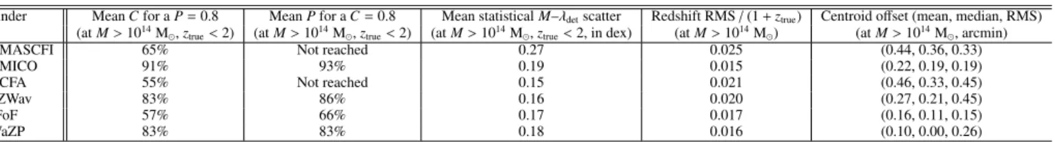
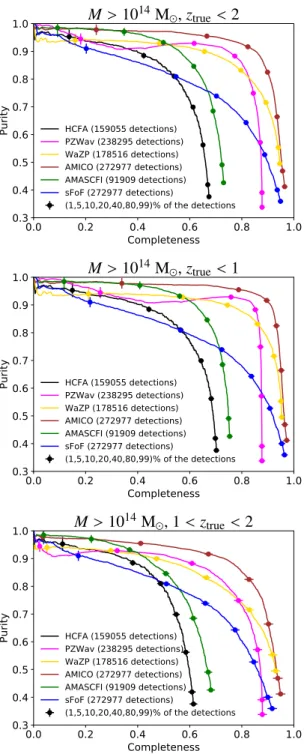
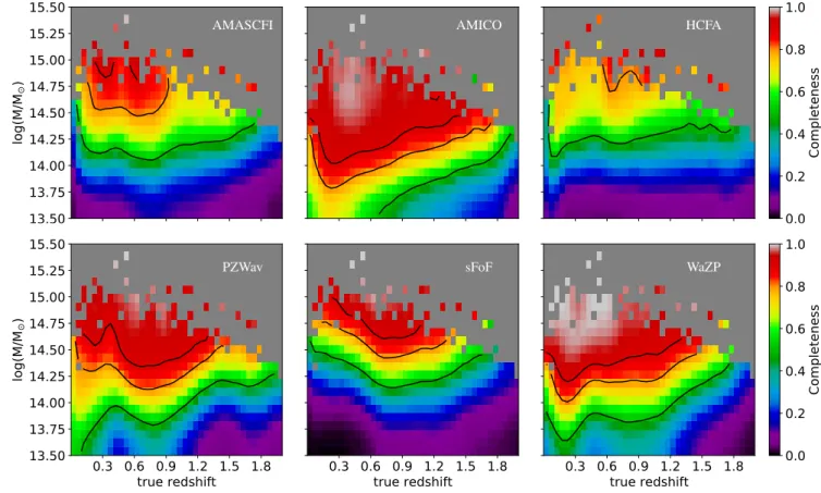
Galaxy cluster counts in bins of mass and redshift have been shown to be a competitive probe to test cosmological models. This method requires an efficient blind detection of clusters from surveys with a well-known selection function and robust mass estimates, which is particularly challenging at high redshift. TheEuclidwide survey will cover 15000 deg2_{of the sky, avoiding contamination by light from our Galaxy and our Solar System} in the optical and near-infrared bands, down to magnitude 24 in theH-band. The resulting data will make it possible to detect a large number of galaxy clusters spanning a wide-range of masses up to redshift∼2 and possibly higher. This paper presents the final results of theEuclidCluster Finder Challenge (CFC), fourth in a series of similar challenges. The objective of these challenges was to select the cluster detection algorithms that best meet the requirements of theEuclidmission. The final CFC included six independent detection algorithms, based on different techniques, such as photometric redshift tomography, optimal filtering, hierarchical approach, wavelet and friend-of-friends algorithms. These algorithms were blindly applied to a mock galaxy catalog with representativeEuclid-like properties. The relative performance of the algorithms was assessed by matching the resulting detections to known clusters in the simulations down to masses ofM200 ∼1013.25M. Several matching procedures were tested, thus making it possible to estimate the associated systematic effects on completeness to<3%. All the tested algorithms are very competitive in terms of performance, with three of them reaching>80% completeness for a mean purity of 80% down to masses of 1014_{Mand up to redshift}

z=2. Based on these results, two algorithms were selected to be implemented in theEuclidpipeline, the Adaptive Matched Identifier of Clustered Objects (AMICO) code, based on matched filtering, and the PZWav code, based on an adaptive wavelet approach.

Key words.Cosmology: observations; large-scale structure of Universe – Galaxies: clusters: general

1. Introduction

Galaxy clusters are good tracers of the matter density peaks in the cosmic web. They additionally provide efficient tests for cos-mological models as they form via gravitational collapse in the expanding Universe (for a review, see Allen et al. 2011). In particular, the number density of galaxy clusters as a function of mass and redshift enables us to constrain cosmological pa-rameters primarily through the linear growth rate of perturba-tions. This has been proven to be very competitive and com-plementary to other probes (e.g., Vikhlinin et al. 2009; Rozo et al. 2010; Planck Collaboration et al. 2014; B¨ohringer et al. 2014;Mantz et al. 2015;Planck Collaboration et al. 2016c;de Haan et al. 2016). The spatial distribution of clusters can pro-vide additional information to help constrain cosmological pa-rameters via the measurement of the cluster-cluster two-point correlation function (e.g.,Majumdar & Mohr 2004;Mana et al. 2013;Veropalumbo et al. 2014;Sridhar et al. 2017). In particu-lar, clusters probe a redshift range that is sensitive to dark energy and hence they can be used to constrain extensions of the stan-dard model. However, any cosmological inference using cluster

?

Corresponding author: R´emi Adam

counts or spatial distribution requires accurate calibration of the halo mass function, an accurate knowledge of the cluster sample selection function, and primary observables that tightly corre-late to cluster masses via scaling relations (including an under-standing of the intrinsic scatter in the scaling relations). The cal-ibration of the proper mass scale is also fundamental for cluster physics studies.

Galaxy clusters can be detected through their hot gas con-tent, either from their X-ray emission (see e.g., B¨ohringer et al. 2001; Pacaud et al. 2016), or using their imprint in the Cosmic Microwave Background (CMB) via the thermal Sunyaev–Zel’dovich effect (tSZ, Sunyaev & Zel’dovich 1972) at millimeter wavelengths (e.g., Hasselfield et al. 2013; Bleem et al. 2015; Planck Collaboration et al. 2016a). In the optical (e.g., Kepner et al. 1999; Rykoffet al. 2014) or near-infrared (NIR; e.g.,Eisenhardt et al. 2008;Wylezalek et al. 2013;Rettura et al. 2014) clusters can be identified using galaxy overdensi-ties. Additionally, optical imaging and analysis methods have now reached the maturity to construct convergence maps via the weak lensing (WL) of background galaxies, where massive clus-ters appear as peaks (e.g.,Gavazzi & Soucail 2007;Shan et al. 2012;Jeffrey et al. 2018). In a cosmological context, the quest for a well-characterized cluster sample, preferably as complete

and as pure as possible, is important in quantifying the likelihood of cluster detections for a given set of cosmological parameters. The properties of galaxy groups and clusters are also essen-tial for understanding galaxy formation because they constitute the local environment in which a significant fraction of galax-ies evolve (see, e.g.,De Lucia et al. 2012;Raichoor & Andreon 2012). Observations show that, at fixed stellar mass, cluster core galaxies present specific properties compared to field galaxies such as lower star formation rates, early-type morphologies and a tight red sequence up to redshift z ∼ 1 (e.g., Mei et al. 2009; George et al. 2011; Wetzel et al. 2013). At higher red-shifts, higher star formation rates are observed in cluster cores as well as more disturbed morphologies (e.g., Brodwin et al. 2013; Alberts et al. 2016; Noirot et al. 2016). A deeper un-derstanding of the mechanisms that trigger such properties and their evolution will be achievable with future large-scale optical or NIR surveys such asEuclid(Laureijs et al. 2011), the Large Synoptic Survey Telescope (LSST,LSST Science Collaboration et al. 2009), the Javalambre-Physics of the Accelerated Universe Astrophysical Survey (J-PAS,Benitez et al. 2014), and the Wide Field Infrared Survey Telescope (WFIRST,Spergel et al. 2015), which will reach cluster masses down to a few 1014 _M

up to

z∼2 (Sartoris et al. 2016;Ascaso et al. 2017). Optical or NIR observation can also potentially select the most massive clus-ters at high redshifts (see e.g., Andreon et al. 2009; Brodwin et al. 2012), and those are likely the place where the first mas-sive galaxies form.

Euclidis a European Space Agency (ESA) mission planned for launch in 2021 that aims at providing a better understand-ing of the origin of the accelerated expansion of the Universe, particularly the nature of dark energy, dark matter, and gravity (Laureijs et al. 2011;Amendola et al. 2013). Through its dedi-cated wide survey,Euclidwill observe 15000 deg2_{, that is a large} fraction of the sky (outside of the Galactic plane), in a wide op-tical band (VIS, down to magnitude 24.5 for a 10σ extended object) and three near-infrared bands (Y,J,H, down to magni-tude 24 for a 5σpoint-source). Deep surveys will cover about 40 deg2_{, which is two magnitudes deeper. Using the Near Infrared} Spectrometer and Photometer (NISP) slitless spectrograph, pho-tometric data will be complemented by spectroscopy, which is expected to release redshifts for several tens of millions of galax-ies. Photometric redshifts that will be obtained by combination with ground based photometric surveys (such as the LSST, J-PAS or the Dark Energy Survey, DES,Abbott et al. 2018) will enable Euclid to detect galaxy clusters over a large range of masses and up to redshift∼2. As an optical and NIR survey, the rest-frame optical richness of clusters will be the natural mass proxy, for whichEuclidwill be able to provide an internal cal-ibration using WL mass estimates and velocity dispersion from spectroscopy using stacking techniques. A recent assessment of

Euclidperformance in terms of weak lensing mass estimates of ensemble clusters (K¨ohlinger et al. 2015) has shown that sta-tistical uncertainties are expected to reach a very low level, and that usually predominant systematic errors such as multiplicative bias and additive bias are expected to be negligible. The richness estimates will also be complemented by other multiwavelength (X-ray, tSZ) mass proxies to reduce systematic uncertainties in the calibration. The combination of these properties should al-lowEuclidto push cluster cosmology to an unprecedented level (e.g., constraints of the order of a few percent on the dynami-cal evolution of dark energy or the growth factor parameter γ, Sartoris et al. 2016).

In order to reach these goals, several cluster finders have been developed within theEuclidconsortium. It was then

neces-sary to develop a work frame to test and evaluate the perfor-mance of these different algorithms in the context of Euclid. Two main methodologies are generally used in the literature, both presenting advantages and limitations: 1) the use of end-to-end simulated data, aiming at matching the expected prop-erties of the real data (e.g.,Koester et al. 2007; Knobel et al. 2009; Adami et al. 2010; Old et al. 2015), or 2) the injection of simulated clusters in a given existing data set (e.g., Adami et al. 2000;Goto et al. 2002;Kim et al. 2002;Rykoffet al. 2014; Planck Collaboration et al. 2016a). Given the rise of multiwave-length data-sets, the comparison of the cluster detections based on different tracers is also now a powerful way to cross-validate the selection functions (e.g.,Saro et al. 2015). On one hand, the first method includes realistic projection effects associated with the spatial correlation between structures, while they are diffi -cult to reproduce using the second method. This is particularly relevant in the case of cluster detection based on the galaxy dis-tribution because the background is expected to be correlated with the targeted objects. On the other hand, the first method relies on the implementation of complex recipes to model the data, while the second method by construction is based on data. The second method is also more flexible regarding the modeling of the simulated cluster. Finally, arbitrary large volumes may in principle be created using the first method, while the second ap-proach requires having in-hand data that are representative of the given survey under consideration, and large volumes to test the detection with sufficient statistics. Recently, the joint use of data and mocks has been shown to be extremely successful to fully account for correlated and uncorrelated background in the deter-mination of richness (Costanzi et al. 2019), demonstrating the benefits of both approaches.

For the purpose of this paper, we use mocks to evaluate and compare the performance of cluster finders. This choice was mo-tivated by several factors: i) mocks allow us to probe the whole redshift range that will be covered byEuclidon a wide-range of richnesses and masses ; ii) they provide the distribution of halos of a given mass and redshift, which can be used as a truth table ; and iii) they preserve the effect of the correlated background. We stress that the main limitation of this approach is the fact that simulations may not fully reproduce all the cluster properties, and the absolute performance derived may therefore be taken with caution. However, we found it the most operational way to compare the relative performance of the different algorithms on a common ground. The full methodology currently developed to determine the selection function and the related mass proxy will be addressed in future work.

The performance of the cluster finder algorithms has been tested and compared in a series of four Cluster Finder Challenges (CFC) between 2013 and 2017. The codes were tested on

in total were tested in the three preliminary challenges, only six of them took part in the final challenge described in this paper.

In this article, we present the methodology used to assess the performance of the codes and the results obtained from the final cluster finder challenge. The detection codes were applied blindly to a realistic galaxy mock, built usingPhotReal(Ascaso et al. 2015) on theEuclidwide light-cone (Merson et al. 2013), which was considered to be the best compromise available in terms of angular size (300 deg2_{), depth (z > 2.5), and realistic} modeling of galaxy properties. We present the main assumptions and methodology of each of the competing codes and discuss the main properties of the simulated mock in the context of cluster detection. The code detections were matched to the true mock clusters and this information was used to evaluate the perfor-mance of the algorithms. Special care was given to the matching procedure by using several methods, allowing us to estimate the associated systematic uncertainties. In light of the mock prop-erties, the performance comparison of the different algorithms participating in the challenge guided our selection of those now being validated and implemented in theEuclidpipeline. At this stage, we stress that the goal of this paper is not yet to compute a robust selection function and robust mass proxies, but instead, to compare the relative performance of different algorithms and to test different methodologies. The definition and assessment of the selection function and the best mass proxies will be ad-dressed in future publications.

This paper is organized as follows. In Section2, we present the competing algorithms. Section3describes the characteriza-tion of the simulacharacteriza-tions that are used. The matching procedure, of associating the detected clusters to the mock clusters, is detailed in Section4, and the performance of the algorithms is given in Section5. We discuss the results and theEuclid algorithm se-lection in Section6. Conclusions are given in Section7. A brief summary of the previous challenges, as well as the description of the previously employed codes are given in the Appendix. Throughout this paper, we assume a flatΛCDM cosmology ac-cording to that used in the mock, withH0 =73 km s−1 Mpc−1,

h = H0/100 km s−1 Mpc−1, Ωm = 0.25, Ω_Λ = 0.75, and

σ8 =0.9. All logarithmic quantities shown in this paper are de-fined using base 10. All the magnitudes in the paper are given in theABsystem.

2. Galaxy cluster detection algorithms

The detection of galaxy clusters from photometric (or spectro-scopic) surveys at optical and NIR wavelengths is a longstand-ing issue (see e.g., the pioneerlongstand-ing work byAbell 1958). Several techniques have been developed, using different kinds of infor-mation. Some algorithms are based on the geometrical distribu-tion of galaxies, both in projected coordinates and in photomet-ric redshift space, while others also focus on known properties of cluster galaxies, such as colors, luminosities, and density pro-files. Cluster finders are generally classified by methodology (or a combination of methodologies), of which a large variety ex-ists in the literature. Some common examples include the use of the cluster red sequence (e.g.,Gladders & Yee 2000;Rykoff et al. 2014), the presence of brightest cluster galaxies (BCG; e.g., Koester et al. 2007), percolation algorithms (e.g., Dalton et al. 1997), matched filtering (e.g.,Postman et al. 1996;Olsen et al. 2007), Voronoi tessellation methods (e.g.,Ramella et al. 2001), friends-of-friends (FoF; e.g.,Wen et al. 2012), the use of smoothing kernel techniques (e.g.,Gal et al. 2003;Mazure et al. 2007), or wavelet filtering techniques (see e.g., the pioneering work ofEisenhardt et al. 2008). These techniques have been

ex-tensively used to build large samples of clusters (e.g.,Gilbank et al. 2011) and have also led to the discovery of some mas-sive clusters at high redshifts (e.g.,Stanford et al. 2012). All de-tection techniques present advantages and drawbacks regarding selection effects, however different techniques are often comple-mentary to one another. For instance, searching for the presence of a red sequence can be an efficient way to detect clusters at low and intermediate redshifts. This property, however, is ex-pected to fade at higher redshifts (e.g., Strazzullo et al. 2016, and references therein) making it less effective for detecting dis-tant clusters. For a review on cluster detection, see for example Gal(2006), or for a detailed discussion about the necessary fea-tures of galaxy cluster finders in the context of large photometric surveys, see for exampleRykoffet al.(2014).

The detection of galaxy clusters in theEuclidsurvey will be largely driven by photometric data. Indeed, analytical estimates (Sartoris et al. 2016) have shown that the mass detection limits obtained using spectroscopic redshifts are significantly higher than those obtained with photometry. Spectroscopic redshifts may also be used to improve the detection procedure, neverthe-less this has not been taken into consideration for this work and is left for future studies. Spectroscopic data will, however, be used to confirm and refine the redshifts of the clusters detected by photometry.

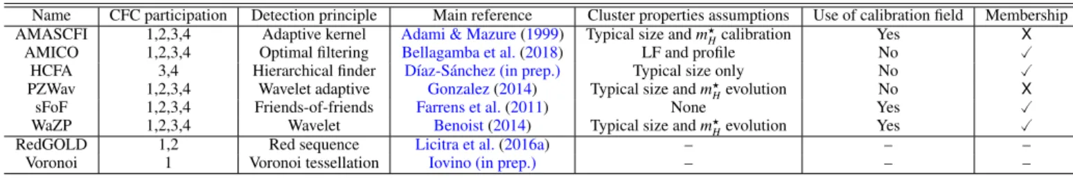
Six algorithms participated in the final CFC. They were all blindly applied to a simulated mock catalog (see Section3) to provide a cluster catalog with the coordinates of the objects (sky coordinates: right ascension, RA, and declination, Dec, and redshift), a mass proxy (typically the richness) and a ranking of the likeliest true detections (mainly by signal-to-noise ratio, S/N). Four algorithms also provided the probability of the clus-ter member galaxies associated with each detected clusclus-ter. The names of the cluster finders, as used hereafter, and their main detection principles are provided in Table1. The following sub-sections provide an overview of the methodology and the as-sumptions used by each code.

2.1. AMASCFI: Adami, Mazure & Sarron cluster finder

Table 1:Summary of properties and names of eight cluster finder algorithms that participated in CFC. The properties listed here correspond to those of the final CFC. All algorithms performed redshift slicing or made use of a grid, and all rely on theH-band in the case of the final CFC. RedGOLD and Voronoi did not participate in the last challenge for reasons not related to their performance in the earlier ones.

Name CFC participation Detection principle Main reference Cluster properties assumptions Use of calibration field Membership

AMASCFI 1,2,3,4 Adaptive kernel Adami & Mazure(1999) Typical size andm?_Hcalibration Yes X

AMICO 1,2,3,4 Optimal filtering Bellagamba et al.(2018) LF and profile No

HCFA 3,4 Hierarchical finder D´ıaz-S´anchez (in prep.) Typical size only No

PZWav 1,2,3,4 Wavelet adaptive Gonzalez(2014) Typical size andm?_Hevolution No X

sFoF 1,2,3,4 Friends-of-friends Farrens et al.(2011) None Yes

WaZP 1,2,3,4 Wavelet Benoist(2014) Typical size andm?_Hevolution Yes

RedGOLD 1,2 Red sequence Licitra et al.(2016a) – – –

Voronoi 1 Voronoi tessellation Iovino (in prep.) – – –

the influence of the choice of parameters can be found inSarron et al.(2018).

The sky coordinates (RA, Dec) and redshift of each candi-date cluster are taken to be the mean of each of its individual merged detections weighted by its galaxy number density. For each redshift slice, the S/N of detected peaks is computed from the 2D density map as (hnclusteriA− hnfieldiA)/

√

hnfieldiA, where

hnclusteri andhnfieldi correspond to the average number density

of galaxies per Mpc2_{in a slice of width∆zfor cluster and field} area, respectively, andAis the cluster area (taken to 500 kpc ra-dius) projected on the sky. For each cluster candidate, the final S/N is taken as the maximum S/N of its individual merged de-tections. The richnessλdetis computed from a modified version of theLicitra et al.(2016a) estimator. AMASCFI first counts the number of galaxies withmH<m?_H+2.5 in a cylinder of radius

Rdet =1 Mpch−1 and length±2σzphot around the cluster center, and removes the galaxy background contribution. The knee mag-nitude of the luminosity function (LF),m?_H, was calibrated using the value measured for the Coma Cluster obtained byde Propris et al.(1998). It then iteratively rescales the detection radius as

Rdet=(λdet(<Rdet)/100)0.2until convergence. For the last CFC, the rank was determined by sorting the S/N values. The richness was used to establish the relative rank for objects with identical S/N values. AMASCFI was applied to the CFHTLS inSarron et al.(2018) and the previous version of the AMASCFI algo-rithm (AMACFI) was used to search for clusters in the CFHTLS (Mazure et al. 2007;Adami et al. 2010;Durret et al. 2011) and in the SDSS Stripe 82 data (Durret et al. 2015).

2.2. AMICO: Adaptive Matched Identifier of Clustered Objects

The Adaptive Matched Identifier of Clustered Objects (AMICO) algorithm (Bellagamba et al. 2011, 2018) is an enhanced matched filter algorithm that looks for cluster candidates by con-volving the 3D galaxy distribution with a redshift-dependent fil-ter. The input of the algorithm is a galaxy catalog that includes sky coordinates (RA, Dec), photometric redshifts and magni-tudes. The filter is defined on the basis of a cluster and noise model that has the purpose of amplifying the contrast between the two components. Originally this filtering method was used to detect galaxy clusters in weak lensing data (Maturi et al. 2005). The noise is modeled by assuming a spatially uniform LF, while the cluster model is the combination of a cluster galaxy LF and a galaxy density profile. In the CFC, AMICO considered only the H-band for detection, but it can use any other magnitude or a combination of two or more. It also accounts for the full shape of the photometric redshift probability distribution func-tion (PDF),P(z), provided by the mock. The convolution of the

galaxy distribution with the AMICO filter generates a 3D ampli-tude map, whose peaks represent the detections. In addition to standard matched filter algorithms, AMICO defines a member-ship probability for each galaxy to belong to a given detection. It uses this information to remove signals in the original amplitude map in order to search for further detections, which might be blended with other structures, without any further assumptions. This has proven to be an efficient method to disentangle close-by objects.

The output sky coordinates (RA, Dec) and redshift of the candidate clusters are given by the position of the peaks in the likelihood on the 3D grid. The uncertainty on the amplitude is derived from the expected variance in the measurement, due to the background fluctuations and the shot-noise in the cluster galaxy distribution. The S/N associated to the candidate clus-ters is then the ratio of the amplitude over its uncertainty. The mass proxy provided by AMICO is the amplitude, a measure of the cluster galaxy abundance in units of the cluster model. Detections are ranked according to their S/N. We note that AMICO can provide another mass proxy, given by the sum of the membership probabilities for each detection (a measurement of the richness, see Bellagamba et al. 2019), but this quantity was not used in this work. AMICO was recently used to iden-tify galaxy clusters in the Kilo Degree Survey (KiDS,Radovich et al. 2017;Maturi et al. 2019).

2.3. HCFA: Hierarchical Cluster Finder Algorithm

The Hierarchical Cluster Finder Algorithm (HCFA) algorithm (D´ıaz-S´anchez, in prep.) searches for overdensities of galaxies using different angular scales in a hierarchical approach. The HCFA algorithm requires only the position and the photometric redshift of the galaxies as inputs. It first uses overlapping redshift bins of size∆z=0.05 (as for AMASCFI) to identify the galaxies that are in local overdensity regions. Each galaxy is then labeled with its local density,ng, according to the galaxies in its neigh-borhood. HCFA uses a primary angular scale of 0.2 Mpc for this purpose. A critical densityngcis defined as 3σngabove the mean local densityDng

E

,ngc=3σng+ D

ng

E

the linking scale reaches 0.6 Mpc. In this way, HCFA identifies galaxy clusters composed of hierarchical overdensities. The al-gorithm uses a sky tiling of 36 arcmin2(chosen for convenience) and tiles are processed in parallel.

The cluster candidate centroids are calculated taking into ac-count all the galaxies in the cluster, while the redshift is given by the mean redshift of the galaxies. A S/N is defined for each galaxy asng−

D

ng

E

/σng. From this definition, the S/N of the candidate clusters are set to the mean S/N of the five galaxies with the highest S/N values in the cluster. A minimum of five galaxies are required in order to define a candidate cluster. The richness is given by the total over-density factor of the cluster, i.e., the number of galaxies in the cluster multiplied by the S/N of each galaxy. The candidate clusters are ranked according to the S/N. The HCFA algorithm has not yet been applied to real data.

2.4. PZWav

The cluster finding algorithm PZWav (Gonzalez 2014) is a wavelet-style algorithm that searches for overdensities on fixed physical scales. PZWav requires a galaxy catalog with sky coordinates, photometric redshifts, and magnitudes. It uses a difference-of-Gaussian smoothing kernel and incorporates for each galaxy the full probability distribution associated with the photometric redshift,P(z). As a preprocessing step, the galaxy catalog is culled to contain only galaxies brighter than a given limit, taken as mH < m?H+2 inH-band, so that galaxies out to z = 1.5 are selected down to the same limit, as traced by any model of galaxy evolution. This preprocessing step mini-mizes the redshift dependence of the mass threshold for clus-ter detection. Afclus-ter this preprocessing is complete, the algorithm first constructs a series of redshift slices spanning the redshift range of interest, and then inserts each galaxy into these red-shift slices, weighted by the probability that the galaxy lies at a given redshift. These density maps are next convolved with a difference-of-Gaussians smoothing kernel of a fixed physical size, which is approximately matched to the physical size of cluster cores. A second set of density maps is also constructed for which the redshift probability distributions have been ran-domly shuffled relative to the positional information. These ran-dom density maps are used for bootstrap simulations to calculate a uniform noise threshold as a function of redshift that is inde-pendent of the mean galaxy density. Galaxy cluster candidates are next identified in each redshift slice, and these detections are merged across the redshift slices. All detections that lie near the edge of the survey field are rejected, and redshift estimates are refined for each cluster using a secondary code that sums the probability distributions of all galaxies within a fixed radius of the cluster detection.

The cluster centroids come directly from the smoothed den-sity maps, corresponding to the peak location of each detected overdensity. Cluster redshifts are derived by computing the

σ−clipped median photometric redshift from all galaxies that lie within 3000_{of the centroid and lie within∆z =0.12 of the} red-shift slice in which a cluster is detected. The direct observable from this search is the peak amplitude of each detected over-density, which can be taken as a proxy for richness. Candidates are ranked by this peak amplitude. The version of PZWav used for the challenges did not calculate the S/N, reporting only the peak amplitude. The current version of the code calculates the S/N based upon the fluctuations in the random maps. This al-gorithm is based upon the approach initially developed for the

IRAC Shallow Cluster Survey (Elston et al. 2006; Eisenhardt et al. 2008), also used in the work ofStanford et al.(2012), but has been optimized and refined to work efficiently withEuclid -like data.

2.5. sFoF: Friends-of-friends

The sFoF algorithm is a friends-of-friends galaxy cluster detec-tion algorithm (Farrens et al. 2011) that follows the principles es-tablished byHuchra & Geller(1982) and later modifications im-plemented byBotzler et al.(2004). The algorithm operates using an input galaxy catalog with either spectroscopic redshifts (3D: using sky coordinates and redshifts) or photometric redshifts (2+1D, as in the present case), using sky coordinates stacked in bins of photometric redshift. All of the internal operations are performed in angular space and no assumptions are made about the nature of clusters of galaxies (e.g., size, color, shape). Two primary free parameters, the transverse linking and the line-of-sight linking lengths, determine the total number of cluster can-didates and their corresponding properties.These linking param-eters change as a function of redshift to account for selection effects, which in turn provides a redshift independent richness estimate for each cluster candidate. The parameters were opti-mized using the calibration field provided with the mock (see Section3). Each FoF group galaxy is marked as a cluster mem-ber and its memmem-bership probability is set to unity, while non cluster members have a membership probability that is set to zero. The code implements k-dimensional tree and Open Multi-Processing routines to improve the performance of a single run. The cluster candidate coordinates (RA, Dec and redshift) are obtained from the median of the member positions. The S/N is computed as (λdet−A nfield)/

√

A nfield, where λdet is the

es-timated richness,Ais the cluster area projected on the sky, and

nfieldis the galaxy background level at the cluster redshift. The

richness is given by the number of FoF objects found for a given cluster, which is also the sum of the membership probabilities. Because the linking parameters change as a function of redshift, this roughly gives a redshift independent estimate. Candidate clusters were ranked according to the richness. The sFoF algo-rithm was applied to the 2SLAQ spectroscopic survey (Cannon et al. 2006) of potential luminous red galaxies inFarrens et al. (2011).

2.6. WaZP: Wavelet Z-Photometric cluster finder

The Wavelet Z-Photometric cluster finder (WaZP) algorithm (Benoist 2014;Dietrich et al. 2014) is an optical cluster finder based on the identification of galaxy overdensities in (RA, Dec,

a statistically rigorous treatment of the Poisson noise, which makes it possible to keep significant structures in an appropriate scale range. Here structures with scales up to 1 Mpc are selected and a 3σiterative multiresolution thresholding with a B-spline wavelet transform is applied. From each wavelet map, peaks are extracted and merged with peaks from consecutive slices to pro-duce a final cluster list.

Each peak detected in the projected filtered maps is charac-terized by i) a position defined as the mode of the peak, ii) a radiusRdetdefined as the mean extent of the peak, iii) a redshift defined as the median redshift of the photometric redshifts se-lected within a projected distance ≤ Rdet from the center and within ±3σzphot around the mean redshift of the map, and iv) a S/N defined as (n− hni)/σbg wheren andhniare the galaxy density within 300 kpc from the peak center and the galaxy lo-cal background density respectively. The quantityσbg is given by the second order moments of galaxy counts in cells. When a cluster is detected in several consecutive slices, it is associated to the peak with the largest S/N. For each cluster, membership probabilities are computed following the prescription given in Castignani & Benoist(2016), based here on a local background density modeling. Membership probabilities are computed up to a radius corresponding to a given galaxy density contrast. Finally each cluster is characterized by a richness defined as the sum of the membership probabilities for galaxies with a magnitude

mH ≤m?_H+1. Clusters are ranked according to their S/N. The WaZP algorithm was applied to N-body simulations inDietrich et al.(2014) and to the CFHTLS data to search for optical coun-terparts to the XXL survey (Pierre et al. 2016) X-ray clusters (Benoist et al., in prep.).

3.Euclid mock galaxy catalog

The finalEuclidCFC made use of a main mock galaxy catalog (Ascaso et al. 2015) in order to test the behavior of the detection algorithms onEuclid-like data. This mock includes photometric redshifts,zphot, and their errors. It was limited toH-band magni-tudes brighter thanHAB=24 to mimic the context of theEuclid wide survey (HAB =24 for 5σpoint-source). A 20 deg2region including both photometric and spectroscopic redshifts was also provided as a calibration field for the photometric redshifts or for the detection code parameters. While it is not the purpose of this paper to make an assessment of the validity of the semian-alytic models on which the mock is based, we do aim to verify the reliability of the model predictions. This is done in order to quantify how realistic the performance of the cluster finders are when applied to the mock. We discuss the construction of the mock in Section3.1.

3.1. Construction of the mock galaxy catalogs

We placed some constraints on the properties of the mock as we aimed to test the performance of the cluster finders at high redshift (up to about 2) and high mass (larger than about 1014 M) in theEuclidregime. In order to satisfy these requirements, the mock has to be complete in magnitude to at leastHAB=24, to cover a redshift range up toz &2, and to have a reasonable sky coverage in order to get enough statistics on the high mass and high redshift clusters. We therefore chose a parent sample of 500 deg2_{from which we extracted a 300 deg}2_{mock. Finally,} this mock was blinded by applying a rotation and translation.

3.1.1. Galaxy catalog

The galaxy catalog was extracted from theAscaso et al.(2015) mock, which was based on the H-band wide light-cone from Merson et al. (2013). The light-cone was generated from the Millennium simulation (Springel et al. 2005) using semiana-lytical modeling of galaxy formation with theGALFORMmodel (Lagos et al. 2012). The mock was reprocessed with the soft-warePhotReal(Ascaso et al. 2015) to obtain realistic galaxy photometry compliant withEucliddepth inY JH(down to mag-nitude 24 at 5σ, point sources) andgrizY(down to magnitudes 25.2, 24.8, 24.0, 23.4 and 21.7 at 10σ, extended sources), as-suming complementary ground-based DES data (Mohr et al. 2012). This corresponds to the pessimistic case inAscaso et al. (2015), as opposed to the combination of theEuclid observa-tions with deeper ground-based photometry from LSST (the op-timistic case inAscaso et al. 2015). In this sense the performance derived hereafter is expected to be conservative.

The photometry was also modified byPhotRealusing a set of empirical templates to fit observed spectral distributions and make the galaxy colors, luminosity and mass functions more consistent with current observations (seeAscaso et al. 2015, for more details). Photometric redshifts were estimated using the Bayesian Photometric Redshifts software (BPZ, Ben´ıtez 2000; Ben´ıtez et al. 2004;Coe et al. 2006) applied to the PhotReal

photometry. The most likely redshifts (PDF peaks) were derived, as well as their probability distribution functions.

We note that the magnitude cut applied to the mock used in the present paper introduces and extra idealization. Indeed, in practice theEuclidcatalog will extend to fainter magnitudes (albeit being incomplete), which may benefit to the detection codes, in particular for the detection of high redshift clusters. In this sense, the results presented in this paper are conserva-tive in terms of performance, as the magnitude cut applied limits the sampling of the luminosity function at high redshift (how-ever still reachingm?+1.5 at redshift 2). In addition, accurate photometry in crowded cluster fields, with the intra cluster light also contributing to the background, is a real challenge as shown in recent studies based on Hubble Space Telescope observations (e.g.,Molino et al. 2017). Such effects, which are not included in the mock used in this paper, may boost the photometric red-shifts uncertainties of the corresponding galaxies, and we leave their detailed investigation for future work, when the end-to-end

Euclid simulations including all observational effects, the final pattern of ground-based complementary observations, and the estimation of photometric redshifts performed with the Euclid

code, will be available.

3.1.2. Mock cluster catalogs

rect-angular area that includes all the galaxies belonging to a given mock cluster.

The mock cluster masses,Dhalo(MDH), were also defined according to Jiang et al. (2014). The MDH values are related to the masses that are generally used in observations, such as

M2001. The median ratio between MDH and M200 is equal to about 1.25 and the distribution remains confined between& 1 and.1.5 at 90% C.L., being fairly flat (Jiang et al. 2014). We note that inJiang et al.(2014), the mass ratio is well character-ized up to MDH '1014 h−1M. Given the smooth evolution of the ratio with mass over several orders of magnitude, we assume that extrapolation is accurate up to the high mass tail considered here,M ∼1015.5_M

. The final mock cluster catalogs were con-structed by selecting all clusters down to masses of 1013.25 M. The implications of this limit on our results is further discussed in sections5and6. Hereafter, the masses are referred asM.

The characteristic radius was estimated as R˜200 ≡

h

M/4₃π200ρc

i1/3

. This quantity is related to the mass of each mock cluster and uses the critical density at the cluster redshift,

ρc, as computed from the mock cosmological parameters in the flatΛCDM model. Because the masses we used are not defined as M200, our estimates of R200 are biased high by around 8% for the median of the cluster population, and remain less than 17% larger at 95% C.L. It should be noted, however, that these

˜

R200values were only used to associate detected clusters to mock clusters and hence this does not significantly affect our results, as discussed further in Section4.

3.2. Properties of galaxies and galaxy clusters in the mocks

To facilitate the interpretation of the results of the final CFC and to validate the simulations for our purposes, we explore the prop-erties of the mock in terms of photometric redshift reconstruc-tion, mass-richness relareconstruc-tion, cluster galaxy density profiles and galaxy cluster LF. An analysis of the galaxy properties in the mock is provided inAscaso et al.(2015). In the following sub-sections we complement this analysis, particularly with regards to cluster environment.

3.2.1. Photometric redshift properties

The precision of the photometric redshift estimates is expected to have a significant impact on cluster finder performance. Clusters appear as overdensities not only in projected space, but also in redshift space, information that is used by the de-tection algorithms via the photometric redshifts. Ascaso et al. (2015) validated BPZ photometric redshifts comparing them to spectroscopic redshifts and assessing their performance in terms of resolution and outliers (see Section 5 of their paper and Tables 1 and 2). We briefly summarize their results and present an internal validation performed in the context of the CFC.Ascaso et al.(2015) showed that for theEuclid pessimistic

caseσNMAD ≤0.03 for galaxymH <22.5 and increases up to

σNMAD ∼0.08 atmH ∼24, using the normalized median abso-lute deviation (NMAD)2. When considering all magnitudes up to

mH=24,σNMAD≤0.045 for redshiftz<1.5 andσNMAD∼0.06 at 1.5 <z < 3. These limits increase when using theodds pa-rameter in BPZ (not used in the CFC). In terms of outliers, the

1 _{The massM}

200 corresponds to the mass enclosed within a radius

R200, within which the mean density of the cluster is equal to 200 times the critical density of the Universe at the cluster redshift.

2 _{The NMAD associated to the variableXis defined asσ}

NMAD(X)= 1.48 median|X−median (X)|.

Euclid pessimisticcase shows a rate of outliers in the range 10-20%, with the highest fractions in the redshift ranges 0.5<z<1 and 2 <z<3. These results are shown inAscaso et al.(2015) Tables 1 and 2 as a function of galaxy magnitude and redshift, and in Figures 17 to 22. As a general comment, the photomet-ric redshift resolution of theEuclid optimistic case is a factor of two to five better than the pessimistic case both in terms of photometric redshift accuracy and bias.

We hereafter present the internal challenge validation of the photometric redshift quality in the simulation. For this, we fol-lowRicci et al. (2018), adapted fromIlbert et al.(2006)3_{. For} each redshift bin, we compute the differencezphot−ztrue, and use the resulting distributions to extract the bias, the catastrophic failure fraction and the dispersion. Here,ztrue refers to the true spectroscopic redshifts. These values account for peculiar ve-locities, which are known for all the galaxies in the simula-tion and are not affected by selection effects. The bias is com-puted as the median of the distribution. The outlier fraction is given by the fraction of objects satisfying

zphot−ztrue−bias

>

0.15 (1+ztrue). The dispersion is computed both using NMAD as inAscaso et al.(2015), and percentiles by integrating the dis-tributions up to a 68.2% confidence level on the positive and negative parts. We also reproduce this analysis after removing galaxies with H-bandmH > 23 magnitude to highlight the ef-fects of contamination from low S/N objects. We note that be-low this limit, the distribution remains fairly stable. Similarly, we reproduce this analysis by selecting cluster member galaxies above a given halo mass, to investigate potential environmental effects.

Figure 1 shows the comparison between the true spectro-scopic redshift, ztrue, and the photometric redshifts zphot, for a randomly selected subsample of galaxies from the mock (∼105 galaxies are shown). This figure also provides the bias and the two estimates of the dispersion. Figure2shows the redshift evo-lution of the catastrophic outlier fraction (top panel), the bias (central panel) and the different estimates of the dispersion (bot-tom panel) for the full mock and after removing objects with

mH>23. The left panel includes cluster and field galaxies while the right panel focuses on cluster member galaxies, belonging to haloes of mass larger than 1014 M. We measure the over-all mean photometric uncertainty to σzphot = 0.050 (1+ztrue). The dispersion increases by a factor of ∼ 2 and becomes very asymmetric at ztrue ∼ 0.5−0.6. It also increases by a similar amount at redshifts below 0.2 and above 2.5 for the full catalog, but remains relatively flat for the high S/N catalog (mH < 23). The bias becomes large where the photometric uncertainties are large, even for themH<23 catalog. The fraction of catastrophic redshifts is small at redshifts above 0.8 (.0.05 even for the full catalog, and about 0.01 for the high S/N catalog). However, it becomes large at lower redshifts, reaching up to 20% for the full catalog and 15% for themH <23 catalog. The distribution remains very similar in the case where cluster member galax-ies are selected, independently of the exact value adopted for the mass cut. We note that the overall quality of the photomet-ric redshifts measured corresponds to the pessimistic case, as expected from the catalog used. In the context of Euclid, the standard deviation of the photometric redshifts with respect to the true redshifts is required to be σz/(1+z) < 0.05, keeping as a goal σz/(1+z) < 0.03 (Laureijs et al. 2011). Similarly, the catastrophic failures requirement is less than 10% beyond

0.15(1+ztrue), while the goal is to keep this less than 5% beyond 0.15(1+ztrue). Our internal validation is consistent with the mock validation performed inAscaso et al.(2015) where a more op-timistic case is also presented in addition to the pessimistic one used here. We note that the large number of outliers, the large bias and the large dispersion at redshifts below 0.3, above 2.3 or near 0.6 are largely due to the fact that nou-band is used in the pessimistic case, while it would be available in the optimistic case.

Based on the photometric redshift properties of the catalog, we expect cluster finder detection properties to be altered in the redshift range in which the catastrophic outlier fraction is large (ztrue ∼ 0.5−0.6, andztrue . 0.2). This is even more true for clusters with fewer member galaxies (i.e., at lower masses). This alteration might show up as an increased number of false detec-tions or larger uncertainties in the redshift recovery of the clus-ters, depending on how the photometric redshifts are used by the finders. The bias can also affect the matching performed to associate the detections to the true clusters (see Section4). At redshifts 0.8<ztrue<2, the photometric redshift distribution is nearly Gaussian (with small bias and a small catastrophic outlier fraction). Therefore, the cluster finders are expected to behave well despite the fact that the larger photometric errors and the lower number of galaxies, reduced by redshift dimming, should impact the completeness.

0.0 0.5 1.0 1.5 2.0 2.5 3.0

z

true

0.0

0.5

1.0

1.5

2.0

2.5

3.0

z

ph

ot

1 to 1 relation

median

1

disp. at 68.2%

Figure 1: Comparison between photometric redshift, zphot, and true spectroscopic redshifts,ztrue. The bias is shown by the purple solid line, the NMAD is shown as the red dashed line, and the dispersion computed as percentiles is shown by the blue solid line. The black dashed-doted line provides the one-to-one relation for reference.

3.2.2. Mass-richness relation

The richness of galaxy clusters is a fundamental quantity derived from optical or NIR surveys. It generally serves as the primary mass proxy and its normalization is tightly related to the detec-tion performance at a given mass. In the context of the CFC, it

was necessary to characterize the mass-richness relation of the mock itself in order to estimate the scatter introduced to richness measurements (see Section5). See also the work byAscaso et al. (2017) for the characterization of the cluster total stellar mass as a cluster mass proxy, using the same mock.

For each mock cluster, we compute an estimate of the rich-ness as the number of galaxies associated to the halo as

λmock=Ngal

mH<m?H,ref(ztrue)+2

. (1)

In order to account for a redshift dependence of the richness def-inition, through the magnitude evolution, we exclude galaxies withmHlarger than m?_H,ref+2. This allows us to have a com-plete sample up tomH = 24 at redshift 2.5 (see also the dis-cussion on the LF in Section3.2.4). The reference magnitude

m?_H,refis derived from the passive evolution of a starburst galaxy with a formation redshiftzform =3 taken from thePEGASE2 li-brary (burst sc86 zo.sed,Fioc & Rocca-Volmerange 1997). It is calibrated using the value ofK?at redshift 0.25 derived by Lin et al.(2006) from an observed cluster sample. The validity of this evolution is addressed in Section3.2.4(see also Figure5, right panel) and the exactm?_H,ref model used to computeλmock has a negligible impact on our results, especially given that it reproduces well the trend seen in the mock at the relevant red-shifts.

In Figure3, we provide an example of the scaling between the mass and the richness, computed for all clusters in the red-shift range [0.5−0.75]. The mass-richness relation is modeled by power law and fitted using the bivariate correlated errors and intrinsic scatter (BCES,Akritas & Bershady 1996) method. The best-fit model is subtracted from the data and the residual is used to compute the scatter in the richness at fixed mass. The blue and purple dots provide the median and mean richness of the corresponding mass bin, while the error bars represent the scat-ter computed as the NMAD and the standard deviation, respec-tively. While the standard deviation is accurate for lognormal scatter, the NMAD is more robust to outliers and we use it as the baseline. The differences between the two methods are insignif-icant. The slope is consistent with unity within a few percent at all redshifts. The scatter does not significantly evolve with redshift (not shown), but it does decrease linearly with logM

(σlogλ'0.1 atM =1013.5Mandσlogλ '0.05 atM =1014.5 M). This intrinsic scatter will be later used when quantifying the scatter introduced by the detection algorithms in Section5. We observe outliers at low richness in the scaling relation when using the mock cluster catalog based on the barycenter of clus-ter galaxies (not shown). They correspond to clusclus-ters that are on the edge of the footprints since their number of member galax-ies is generally truncated while their mass remains the same. In principle, these clusters also affect the detections, but we have observed that they have a negligible impact on the global perfor-mance presented in this paper. In practice, theEuclidsurvey will be affected by masks, or varying depth, but at this stage not all the algorithms are able to handle such effects and we leave the investigation of their impact on the detection of galaxy clusters for future work.

3.2.3. Cluster galaxy density profile

0

10

20

f

/(1

+

z

) (

%

)

all catalog

mH< 23

2.5

0.0

2.5

10

2

b/

(1

+

z

)

0.0

0.5

1.0

1.5

2.0

2.5

z

0.0

0.1

0.2

/(1

+

z

)

68.2% CL up 68.2% CL low

0

10

20

f

/(1

+

z

) (

%

)

Mhalo> 1014.0 M mH< 23

2.5

0.0

2.5

10

2

b/

(1

+

z

)

0.0

0.5

1.0

1.5

2.0

2.5

z

0.0

0.1

0.2

/(1

+

z

)

68.2% CL up 68.2% CL low

Figure 2:Redshift evolution of the catastrophic outlier fraction (fc, upper panel), the bias (b, middle panel), and different estimates of the

disper-sions (σ, lower panel) as a function of spectroscopic redshift. The solid lines correspond to the full catalog, while the dashed lines correspond to the catalog once objects fainter than magnitudemH =23 are removed. Upper and lower values of the dispersion computed using percentiles with

respect to the de-biased distributions are shown according to the legend. The left panel provides the distributions for the field plus cluster member galaxies and the right panel focuses on cluster member galaxies, i.e., those within haloes more massive than 1014_M.

13.6 13.9 14.2 14.5 14.8 15.1 15.4

log M/M

0.0

0.5

1.0

1.5

2.0

2.5

3.0

log

tru

e

0.5 < z

true

< 0.75

BCES (Y|X)

individual clusters

1 (standard dev.)

1 (NMAD)

Figure 3:Example of the mass-richness scaling, for the redshift range

ztrue =[0.5,0.75]. The red dots show the cluster population. The blue points with error bars represent the median richness and scatter com-puted as the normalized median absolute deviation, while the purple points correspond to the mean richness and the scatter computed as the standard deviation within each bin.

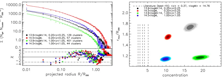
number density distribution of the clusters,Σ(R). We therefore investigate the projected radial profiles of the mock clusters by stacking galaxies belonging to clusters in mass and redshift bins. Prior to the stacking, we normalize the projected clustercentric distances by the characteristic radiusR200.

In order to study in a quantitative way the mass and redshift evolution of the profiles and compare it to observations from the literature, we use the following approach. We model the pro-files by a Navarro, Frenk and White (NFW,Navarro et al. 1996) distribution, as expected from observations (e.g.,Carlberg et al. 1997;Lin et al. 2004). However, as we observe a deficit of galax-ies in the outskirts of the profiles, we also include a truncation radius,rmax, above which the number density of galaxies is set

to zero. The 3D profile of the cluster galaxy space density,n, can thus be written as

n(r/R200)=

n0

(c r/R200) (c r/R200+1)2

H(rmax−r), (2)

whereH is the Heaviside step function, n0 the normalization,

c = R200/rc the concentration, with rc a characteristic radius, andrmaxa truncation radius. We fit the stacked normalized num-ber surface density profiles,Σ(R), as described by equation (2), using the analytical projection given in Mamon et al. (2010). The parameter space (normalizationn0, number concentrationc, and truncation radiusrmax) are sampled using a Markov Chain Monte Carlo method, using the algorithm described in Adam et al.(2015).

The left panel of Figure4provides the stacked projected pro-files of clusters in four redshift and mass bins together with the best-fit models. Overall, the clusters are relatively well described by a truncated NFW model. However, some excess is seen above the best-fit truncation radius, probably due to the fact that each cluster may present a slightly differentrmaxvalue, while we are introducing blurring in the profile when stacking and only fitting for a unique rmax/R200. In addition, the mock clusters present a significantly shallower slope in the center. The best fits are thus slightly biased high in the center, and biased low in the in-termediate regions, as seen in the residual. The right panel of Figure4gives the marginalized posterior likelihood for the pa-rameterrmaxversusc. The truncation radius decreases with red-shift, beingrmax/R200 ∼1.1−1.8. Such a trend could be due to the fact thatrmaxmeasures more closely the virial radius, which is defined at higher densities at higher redshifts, leading to radii that will be smaller. However the size of the effect we find is larger than expected. This truncation is not expected from obser-vations, which indicate that the intrinsic cluster number density profile (not counting galaxies in other groups for clusters) ex-tends to over ten virial radii (Trevisan et al. 2017).

The number concentration parameter, is c ∼ 10 at high masses (> 1014.5 M) and increases up to 20 at lower masses (about 1013.9_M

estimated fitting radial number density and stellar mass density profiles of satellite galaxies in observed massive clusters by a factor of about two or more, depending on mass and redshifts (Carlberg et al. 1997;Lin et al. 2004;Collister & Lahav 2005; Muzzin et al. 2007;van der Burg et al. 2014,2015;Cava et al. 2017). Some of these observational values of concentration and truncation radius (normalized toR200) are reported in the right panel of Figure4, showing a significant offset with respect to the values estimated from the mock. This discrepancy is simi-lar to that found byBudzynski et al.(2012) comparing number density profiles estimated from SDSS DR7 groups and clusters and predicted profiles from semianalytical modeling of galaxy formation. Indeed, the treatment of the galaxy mergers in the model is shown to impact on the profile shape. When a galaxy becomes a satellite, an analytic estimate of the merger time is made and the galaxy merges regardless of whether or not its host sub-halo can still be resolved. According to the way this merger dynamical timescale is calculated may lead to steeper in-ner satellite number density profiles in the case of semianalytic models as compared to observed ones. Our main concern here is if this difference could hamper our performance estimation of cluster finders.

As highly concentrated clusters are expected to be more eas-ily identified by cluster finders, this high concentration poten-tially affects the detections. This may boost high the absolute estimate of the performance, in particular for low S/N objects. However, all the cluster finders are density-based, so their rel-ative performance should not be affected by the higher concen-trations. In addition, the truncation of the simulated clusters at 1 to 2R200facilitates the distinction of the cluster with the back-ground galaxy density, helping the cluster finders limit the di-mensions of the clusters on the sky. However, this effect is likely to have a minor impact on the results because the truncation hap-pens at large radii and only marginal effects are visible in the inner part of the clusters once projected along the line of sight.

3.2.4. Cluster galaxy luminosity function

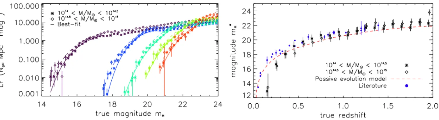
Another important cluster property which can a priori affect its detection is its luminosity function. If the galaxy luminos-ity function in the mock clusters was significantly different from that of the real data, this may impact on the estimate of the ab-solute performances of the cluster finders. We note however that this is not of major importance for this analysis, in which we are mostly interested to the relative properties of the cluster finders. We follow the same approach as for the profiles in order to investigate the LF of galaxy clusters within the simulations (see alsoAscaso et al. 2015, where the mock galaxy luminosity and mass functions were shown to be in good agreement with ob-servations). We count the number of cluster galaxies in bins of magnitude (in theH-band prior to introducing any noise on the galaxy fluxes), within a projected radius ofR200and per Mpc2. This is done after selecting clusters within bins of mass and red-shift. The LF is then fitted by a Schechter function (Schechter 1976), given by (see e.g.,Driver et al. 1994)

Φ(m)=0.4 log (10)φ?100.4(m?−m)(α+1)exp−100.4(m?−m). (3) As in the case of the galaxy density profile, we fit for the pa-rametersφ?,m?, andα, which set the normalization, the char-acteristic magnitude, and the faint-end slope of the population, respectively. Several observational estimates of the cluster LF have shown that a single Schechter function may not reproduce well both the bright and the faint part of the LF, for various rea-sons (e.g.,Popesso et al. 2005;Barkhouse et al. 2007;Yang et al.

2008;Trevisan & Mamon 2017). However it can be used suc-cessfully to model its bright part. Here, the Schechter function is not able to describe the mock LF in the faint part (typically

m > m?+3), where a more sophisticated modeling would be necessary. Therefore, we first focus on the bright end of the LF studying the evolution of the parameter m?. To do so, we per-form the fit of equation (3) in the magnitude range limited to

mbrightest+3, where mbrightest is the magnitude of the brightest

galaxy in the bin we consider. This ensures good modeling of the mock LF in this regime. We check that our best-fit is not sensitive to this magnitude limit. The faint end properties of the LF are addressed as a function of redshift without relying on a model.

The left panel of Figure5provides the cluster galaxy LF in two bins of mass (above 1014_M

) and five redshift bins (among the twenty considered, fromz = 0 to 2). We observe that the mock LF are well described by the Schechter function in the bright regime, but that the faint part may require more sophisti-cated modeling. The right panel of Figure5compares the evo-lution of the best-fitm?parameter to a passive evolution model derived fromFioc & Rocca-Volmerange(1997), as well as from data taken from the literature. The blue points indicatem?_H val-ues fromde Propris et al.(1999);Nakata et al.(2001);Ellis & Jones(2004);Lin et al.(2004);Toft et al.(2004);Andreon et al. (2005);Strazzullo et al.(2006);Muzzin et al.(2007);Strazzullo et al.(2010);De Propris(2017). They were obtained from stud-ies of K-band cluster luminosity functions at different redshifts. We converted them?_K values to the H-band using the early-type k-corrections ofMannucci et al.(2001) and the mean rest-frame color for cluster galaxies,mH−mK =0.26, obtained as an aver-age of the values provided byBoselli et al.(1997);de Propris & Pritchet (1998); Ramella et al. (2004), and adopting when needed the transformation to the AB-systemmHAB =mH+1.37 (Ciliegi et al. 2005). The evolution of the mock is relatively well described by the model and matches well the literature data at redshift larger than 0.3, for the two mass bins considered, but the value of m? is overall lower by about 0.5 magnitude for the passive evolution model. At lower redshifts, the evolution is stronger with redshift and the mockm?values are lower than the model and the literature values.

We have also investigated if the performance of the cluster finders could be affected differently according to the way the lu-minosity function is used in the detection process. While sFoF and HCFA algorithms do not make use of the luminosity func-tion, AMASCFI, AMICO, PZWav and WaZP do. In the case of AMICO, the procedure adopted is fully general and treats the mock as real data. The procedure starts from an initial simple model (built in a blind way) with a luminosity function extracted from all galaxies in the catalog. AMICO is run to define a first set of detections that have been used to refined the cluster model, now introducing a different LF for clusters and field. Finally, AMICO is run with this refined model to derive the final cata-log. In the case of PZWav and WaZP, a value ofm?derived from passive evolution model is used to define a constant stellar mass threshold with redshift for detection. However, the dependance of the performance on them?cut was tested and found to be neg-ligible. AMASCFI, PZWav and WAZP also usem? parametriza-tion for richness estimaparametriza-tion, but here again richnesses are only used as relative quantities. Therefore, the impact of different uses of the luminosity function by the cluster finders is expected to be negligible on their relative performance.

Figure 4:Left:stacked surface density (projected) profile of cluster galaxies. The different colors indicate different mass and redshift bins, as

indicated in the legend. The solid lines provide the best-fit models of equation (2) in each case. The residual normalized by the error, χ, is also provided.Right:posterior likelihood on the model truncation radius parametersrmaxand concentrationcfor each bin, providing the 68%, 95% and 99% C.L. The vertical dashed lines represent the best-fit number concentration cluster observational data from the literature, namely:

c = 2.90±0.22 (at a median redshift med(z) = 0.04, and median mass med(M200) = 4×1014_{M,Lin et al. 2004),c = 4.13±0.57 (at} med(z) = 0.31, med(M200) = 3×1014_{M,Muzzin et al. 2007),c = 5.14}+0.54

−0.63(at med(z) = 1.00, med(M200) = 2×10

14_{M,van der Burg}

et al. 2014), 1/c=0.278±0.065 (at med(z)=0.06, med(M200) =6×1014_{M,van der Burg et al. 2014),c=2.40±0.30 (at med(z) =0.44,} med(M200)=14×1014_{M,Annunziatella et al. 2014).}

The BCG is coincident with the central galaxy in about 70% of the clusters. This number increases with mass, reaching nearly 100% for the most massive clusters. When the BCG is not the central galaxy, the distance from the BCG to the cluster cen-ter (either defined as the central galaxy or the barycencen-ter), is about 0.45R200, decreasing by a few percent as mass increases. However, the distribution extends up to around 2R200in the low mass clusters. Even when it is not the BCG, the central galaxy is among the brightest members and the magnitude difference with the BCG does not exceed∆mH ∼2, or∆mH ∼0.5 at high mass. The differences between the BCG and the central galaxy can affect the cluster finders to some extent, but we note that no finder relies on the BCG directly. As discussed in Section4, the associations between the detection based on the BCG and the clusters in the mock could even be missed in a small fraction of the cases, but we have verified that this does not significantly impact the results. We have also checked that the distribution of halo BCG magnitudes in the mocks was in good agreement with observations.

Another important property of the galaxy distribution to be fiducially reproduced by the mocks is the color distribution. We do not focus on that point in this paper since none of the cluster finders participating in the last CFC was relying on galaxy col-ors. We refer to the work byAscaso et al.(2015) who found a good agreement in the red sequence properties and the blue val-ley location between mocks and observation in the redshift range [0.3,1.65].

4. Mock cluster to detected cluster associations

The assessment of the performance of an algorithm requires as-sociating the candidate clusters and the mock clusters, which are known from the simulation (see e.g.,Knobel et al. 2009, and in particular their Figure 3). In this section, we present the method-ology developed to perform this association as well as an esti-mation of the corresponding systematic effects.

4.1. Matching procedures

The association between candidate clusters and mock clusters, or any pairs between cluster catalogs, is a non-trivial task. In order to validate our methodology and test for systematic effects, we have developed three different matching methods. They are here-after referred to asgeometrical,ranking, andmembership

matching. The matching can generally be performed in two ways, starting from the mock clusters and searching for asso-ciated detections, or starting from the candidate clusters and searching for counterparts in the mock. We define the one-way associations as the clusters for which the association has been made in one direction, but not the other one. Similarly, we define the two-way associations as the ones for which the associations are bijective.

4.1.1. Geometrical matching

Thegeometricalmatching method is implemented via the fol-lowing steps.

1. For each mock cluster, we search for detection counter-parts within a volume around the mock cluster. The volume depth along the redshift axis is controlled by the parameter

∆zmatch=kσ0(1+z) whereσ0=0.05 (see Section3.2.1). We

re-Figure 5:Left:stacked LF of cluster galaxies. The different colors indicate different redshift bins, of width 0.1, used to compute them. Only

redshift bins centered on 0.15 (purple), 0.55 (blue), 0.95 (cyan), 1.35 (green) and 1.75 (red) are shown for clarity. As indicated in the legend, the star and diamond symbols correspond to the two mass bins, in the range 1014₋₁₀14.5_{Mand 10}14.5₋₁₀15_{M, respectively. The solid and dashed} lines provide the best-fit models of equation (3) in the bright magnitude regime, in the low and high mass bins, respectively. We note that in the high mass bin, the number of clusters per bin may be less than 10 at redshifts larger than 1.5, and reaches 2 in the last bin.Right:redshift evolution of the parameterm?_H, for each mass bin using similar symbols, and comparison to the passive evolution model, as the red dashed line, fromFioc & Rocca-Volmerange(1997), and calibrated using the work byLin et al.(2006). The blue points indicatem?_Hvalues from the literature (see text). The error bars provide the standard deviation of the posterior distribution of the parametersm?_H, but we stress that the distributions are generally non gaussian and non symmetric (seeRicci et al. 2018, for a detailed discussion on this topic).

stricted to be withinθ200of the mock cluster, the angular ra-dius corresponding toR200, given the mock cosmological pa-rameters. In the case of massive and nearby clusters, this last condition is more restrictive than the first one. However, as redshift increases and mass decreases, the number of cluster galaxies remaining above the mock flux limit drops, and for a given cluster, all the mock cluster galaxies are eventually enclosed withinθ200. In this case, this secondary constraint becomes ineffective with respect to the first one.

2. In the case of multiple counterparts within the volume, we define the matched cluster as the one which is the closest (projected on the sky) to the mock cluster. Nevertheless, we record the total number of possible matches for all mock clusters, as they correspond to fragmented detections. 3. We repeat the first step (search for counterparts in the volume

around the cluster), using the candidate clusters as the refer-ence and searching for mock counterparts. While the redshift criterium is symmetric and remains the same, it is not the case for the projected area because the detection algorithms do not provide a characteristic radius of the detected objects. Therefore, a mock cluster is associated with the detection if it is at a projected distance that is lower than its ownθ200. 4. We repeat step 2 with candidate clusters as the reference. 5. By comparing mock and cluster detection counterparts, we

identify mock clusters and detected clusters for which the association is identical both ways.

This method allows us to define both the one-way and the two-way associations. In case a mock cluster is associated with a multiple number of detections, this indicates that fragmenta-tion has occurred and this is an important quality assessment of a cluster finder. Similarly, detected clusters that are matched to multiple mock clusters correspond to over-merging events. The two-waygeometrical matching is taken as the baseline method in the present paper.

4.1.2. Ranking matching

Therankingmatching method follows the same initial condi-tion as thegeometricalmatching (first step: search for coun-terparts in the volume around the cluster). However, instead of

performing the matching both ways, it associates candidate clus-ters to mock clusclus-ters after ranking them by decreasing mass, as provided from the mock catalogs, and richness, as provided by the cluster finders, respectively. The richest detected clusters are then matched to the most massive mock clusters, and subse-quently removed from the list. If two or more clusters have the same richness within the association volume, the nearest one to the mock cluster center is selected. Because detected and mock clusters are subtracted from the cluster list as they are matched to one another, this matching procedure is bijective by construction and thus corresponds to a two-way matching. It cannot, there-fore, be used to address fragmentation and over-merging issues. Therankingmatching follows the idea that the most massive clusters, i.e., the richest ones, are the first ones detected.

4.1.3. Membership matching

Thegeometricalmatching and therankingmatching do not directly rely on the cluster member galaxies. In contrast, the third method we developed, hereaftermembershipmatching, consists in defining the associations using the galaxies that are detected as cluster members by the algorithms. Because not all the de-tection algorithms provide the galaxy membership information, this method is only used as a crosscheck (see Table1for the al-gorithms that provide the membership). The main steps of the procedure are summarized as follows.

1. For each mock cluster, we search for detection counterparts within the volume as defined in the case of thegeometrical

matching.

2. If matches are found, we define the fraction of common galaxies between the candidate cluster and the mock clus-ter, with respect to the mock cluster (i.e., the success rate) as

fcom,mock =

P

iPmatchi

Ngal,mock

, (4)

wherePmatch