THREE
ESSAYS IN
MACROECONOMICS
Calebe de Oliveira Figueiredo
A dissertation submitted to the faculty of the University of North Carolina at Chapel Hill in par-tial fulfillment of the requirements for the degree of Doctor of Philosophy in the Department of
Economics.
Chapel Hill 2019
Approved by:
Neville Francis
Riccardo Colacito
Eric Ghysels
Lutz Hendricks
c
2019
ABSTRACT
CALEBE DE OLIVEIRA FIGUEIREDO: Three Essays in Macroeconomics. (Under the direction of Neville Francis)
I extract a global factor from cross-country output growth and find that its fluctuations are typ-ically small, with unconditional volatility estimated at0.06%, but highly persistent, with estimated persistence at0.99. The data indicate that the volatility of the global factor varies over time and that these movements in global macroeconomic risk are an important driver of international business cycles. My empirical results suggest that the exposure to the global factor is not homogeneous across countries and such heterogeneity enables countries to share global volatility risk. I propose a theoretical framework in which agents fear model misspecification can successfully replicate the volatility-driven dynamics observed in the data.
The most recent recessions in Brazil pose a challenge for current business cycle models owing to a key piece of legislation that causes labor to adjust in unconventional ways. We propose a two sector model that resembles the formal and informal sectors in Brazil with the former subject to a termination penalty inspired by said legislation. The informal sector, however, makes labor decisions in a frictionless environment. Our model accurately predicts that recessions preceded by long expansions impact labor levels more severely than downturns following shorter economic booms. Also, the state dependence property of our adjustment cost allows us to replicate the delay between the beginning of an economic downturn and the trough in the formal-sector labor level, a feature observed in the 2014-2016 depression in Brazil.
ACKNOWLEDGMENTS
I am deeply indebted to my advisors Neville Francis and Riccardo Colacito who have been out-standing mentors. Their guidance made this dissertation possible.
I am also grateful to the members of my committee, Eric Ghysels, Lutz Hendricks and, in particular, Stan Rabinovich for the insightful comments and suggestions that improved my research considerably.
TABLE OF CONTENTS
LIST OF TABLES . . . ix
LIST OF FIGURES . . . x
1 Global Long-run Risk and International Business Cycles: A Factor-Stochastic Volatil-ity approach . . . 1
1.1 Introduction . . . 1
1.2 Empirical evidence . . . 3
1.2.1 Data . . . 4
1.2.2 Factor-Stochastic Volatility: Specification and Identification . . . 5
1.2.3 Estimation and results . . . 7
1.2.4 Global volatility risk sharing: VAR evidence . . . 9
1.2.5 Impulse-responses and interpretation . . . 12
1.2.6 Economic implications of factor dynamics . . . 14
1.3 Discussion . . . 17
1.3.1 Robust disagreement . . . 21
1.4 Theoretical framework . . . 22
1.4.1 Model solution: pseudo-Pareto weights and optimal allocations . . . 24
1.4.2 Macroeconomic prices: terms of trade, exchange and interest rates . . . 25
1.4.3 Global volatility-risk sharing: replicating empirical impulse-responses . . . 31
1.5 Concluding remarks . . . 33
2.1 Introduction . . . 35
2.2 Motivation . . . 38
2.3 Labor adjustment costs in Brazil: legal background and economic implications . . . 39
2.4 The model . . . 41
2.4.1 Workings of the model . . . 44
2.4.2 Labor dynamics . . . 45
2.4.3 The household’s problem . . . 47
2.4.4 Stochastic processes . . . 50
2.5 Empirical methodology . . . 51
2.5.1 Data . . . 52
2.5.2 Parameter estimation . . . 53
2.6 Discussion . . . 56
2.6.1 The economy before 2003 . . . 58
2.6.2 The 2008 Financial Crisis . . . 62
2.6.3 The 2014-2016 depression: the role of state-dependent labor adjustment cost . . . 65
2.7 Conclusion . . . 68
3 Worker Reallocation with Tenure-Dependent Labor Severing Costs: A Life-Cycle Perspective . . . 70
3.1 Introduction . . . 70
3.2 Motivation . . . 72
3.3 Empirical Considerations . . . 74
3.4 The Model . . . 78
3.4.1 Model Framework . . . 78
3.4.2 Firms . . . 79
3.4.4 Wage Determination . . . 81
3.4.5 Worker Flows . . . 82
3.5 Results . . . 83
3.6 Conclusion . . . 88
A Appendices . . . 89
A.1 Chapter 1: Model . . . 89
A.1.1 Preference for robustness . . . 89
A.1.2 Solution to the planner’s problem . . . 91
A.1.3 Exchange rate and stochastic discount factors . . . 93
A.2 Chapter 3: Model Solution . . . 94
A.3 Figures . . . 98
A.4 List of Tables . . . 106
LIST OF TABLES
A.1 Prior distributions for the Factor-Stochastic Volatility model. . . 106
A.2 Estimates for the Factor-Stochastic Volatility model described in Eq. 1.1. Posterior means and90%credible bounds shown. . . 107
A.3 Credibility intervals for exposure to Europe and BRICS factors. . . 108
A.4 Calibrated parameters. . . 108
A.5 Estimated structural parameters. Gamma priors: mean and standard deviation in parenthesis. Uniform priors: support lower and upper bounds in brackets. Posterior means and90%credible intervals displayed. . . 109
LIST OF FIGURES
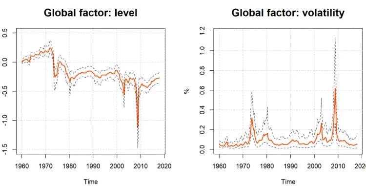
A.1 Filtered values for the global factor of output growth. Percentiles 0.05, 0.5 and
0.95of posterior distributions shown. Annualized volatility in the right panel. . . . 98 A.2 Filtered values for the BRICS factor of output growth. Percentiles 0.05, 0.5and
0.95 of posterior distributions shown. Annualized volatility in the right panel. BRICS countries: Brazil, Russia, India, China and South Africa. . . 98
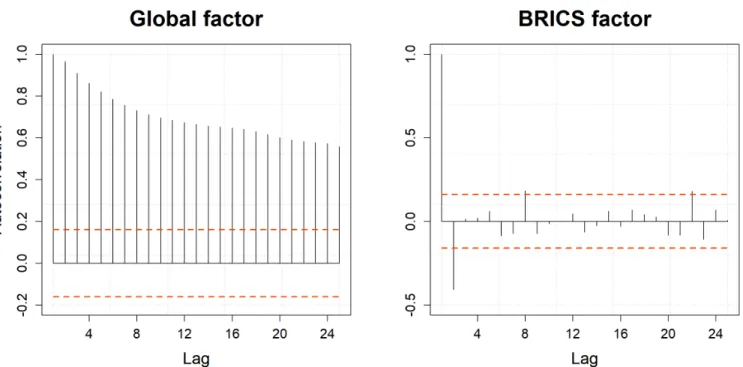
A.3 Empirical autocorrelation functions of the global and BRICS factors. . . 98
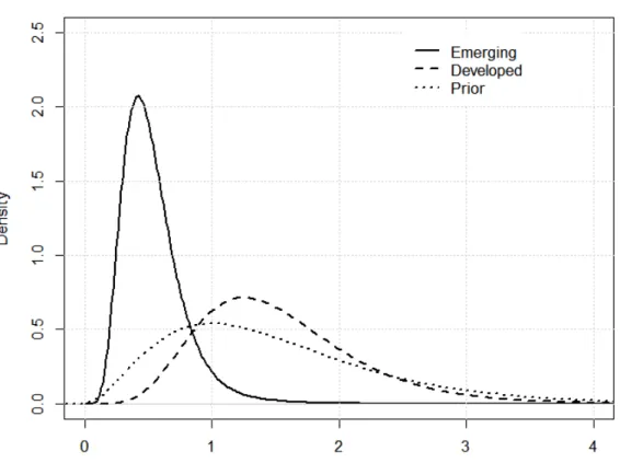
A.4 Precision of exposure to global factor. Prior distribution (dotted) and posteriors for emerging (solid) and developed (dashed) countries. . . 98
A.5 Density plots of prior (dashed line) and posterior (solid line) distributions. . . 98
A.6 Posterior draws of the exposure to the global factor. 90%credible bounds shown. Cutoffβ = 0shown in dashed line. Exposure for the U.S. set at1so unconditional log-variance is identified. Countries with exposure significantly greater than zero are assigned to the high-exposure group. The remaining countries are deemed to have low exposure. . . 99
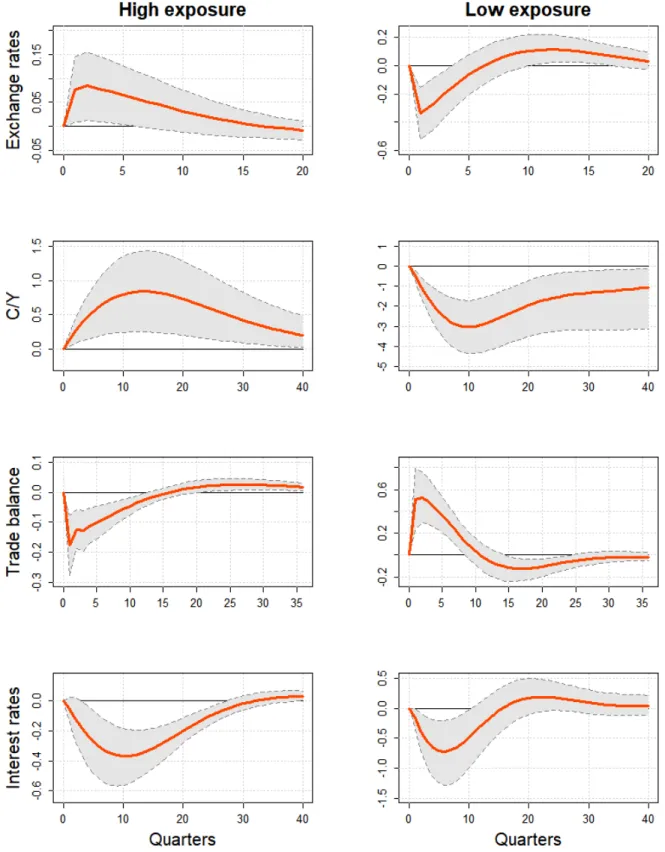
A.7 Responses to a1-s.d. shock to the volatility of the global factor. Structural shocks identified via Cholesky decomposition of residuals’ covariance matrix. Bayesian VAR(1) estimated with flat-Normal prior for autoregressive coefficients and inverse-Whishart for residuals’ covariance matrix. Vector ordering: exchange rate growth, consumption-output ratio, trade balance growth, global factor level (posterior mean), global factor volatility (posterior mean). . . 100
A.8 Responses to a1-s.d. shock to the volatility of the global factor. Structural shocks identified via Cholesky decomposition of residuals’ covariance matrix. Bayesian VAR(1) estimated with flat-Normal prior for autoregressive coefficients and inverse-Whishart for residuals’ covariance matrix. Vector ordering: global factor volatil-ity (posterior mean), global factor level (posterior mean), exchange rate growth, consumption-output ratio, trade balance growth. . . 100
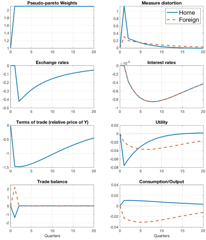
A.10 Impulse-responses implied by model economy. Responses to a1-s.d. shock to the volatility of global factor. ’Measure distortion’ denotes the additional probability weight assigned to high-volatility state - quantitatively identical to marginal utility e−θ Ui,t+1/E
t e−θ Ui,t+1
. Preference for robustness parameter set at θ = 15. Mod-erate home bias in consumption: α = 0.95. Heterogeneous exposure to global factor:βh = 1.2andβf = 0. . . 100 A.11 Impulse-responses implied by model economy. Responses to a1-s.d. shock to the
volatility of global factor. ’Measure distortion’ denotes the additional probability weight assigned to high-volatility state - quantitatively identical to marginal utility e−θ Ui,t+1/E
t e−θ Ui,t+1
. Preference for robustness parameter set atθ= 15. Strong home bias in consumption: α = 0.98. Heterogeneous exposure to global factor: βh = 1.2andβf = 0. . . 101 A.12 Impulse-responses implied by model economy. Responses to a1-s.d. shock to the
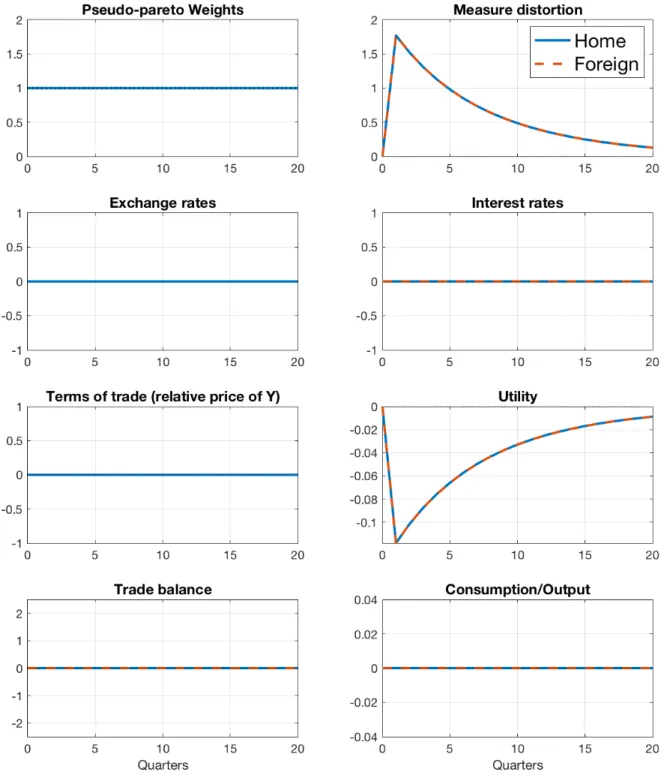
volatility of global factor. ’Measure distortion’ denotes the additional probability weight assigned to high-volatility state - quantitatively identical to marginal util-ity e−θ Ui,t+1/Et e−θ Ui,t+1. Preference for robustness parameter set at θ = 15. Moderate home bias in consumption:α = 0.95. Homogeneous exposure to global factor:βh = 1.2andβf = 1.2. . . 101 A.13 Impulse-responses implied by model economy. Responses to a1-s.d. shock to the
volatility of global factor. ’Measure distortion’ denotes the additional probability weight assigned to high-volatility state - quantitatively identical to marginal utility e−θ Ui,t+1/Et e−θ Ui,t+1. Preference for robustness parameter set at θ = 15. No home bias in consumption: α = 0.5. Heterogeneous exposure to global factor: βh = 1.2andβf = 0. . . 101 A.14 Response of interest rates to a1-s.d. shock to the volatility of the global factor. . . 101
A.15 Quarterly GDP growth and formal-sector labor index. Formal-sector index is work-force employed in production of manufactured goods in the S˜ao Paulo state. Source: FIESP - Federation of Industries of the State of S˜ao Paulo. . . 101
A.16 Labor level and real wage in the formal and informal sectors. Deviations from steady state. Shaded areas indicate economic recessions. . . 102
A.17 Output, consumption, and investment. Deviations from steady state. All variables are measured in real terms. Shaded areas indicate economic recessions. . . 102
A.18 Unfiltered data measured in Brazilian Reais (R$) of 12/2017 (log scale). Top panel: aggregate FGTS deposits. Bottom panels: average wage in formal and informal sectors. . . 102
A.20 Empirical density plots of prior and posterior distributions of adjustment cost pa-rameters. . . 102
A.21 Empirical density plots of prior and posterior distributions of preference and pro-ductivity processes parameters. . . 102
A.22 Model-implied impulse responses. System is at steady state att = 0 and a1s.d. shock to long-memory TFPεm
t arrives att= 1. Aggregate investment in physical capital and savings rate are lower under the labor adjustment cost implied by the FGTS policy relative to a standard frictionless economy. Capital allocation shifts towards the informal sector. . . 103
A.23 Model-implied impulse responses. System is at steady state att = 0 and a1s.d. shock to long-memory TFPεm
t arrives att = 1. Employment and wage growth in the formal sector is partially hampered by the adjustment cost. While lower wages incentivizes higher employment, wage is only the direct price of labor in the model. The indirect price of labor, denoted byλH, rises as as the labor increases and the result of these opposing forces generate the dynamics of formal-sector labor. The wage wedge, which is defined as the difference between wage and marginal product of labor, declines sharply as the economy improves, indicating that the productivity gains are not promptly transferred to workers. . . 103
A.24 Recovery from the 2002 recession. Low employment in the period leading up to the 2002 recession entailed low aggregate FGTS holdings when the economy recov-ered. The small termination penalty under the FGTS specification allowed enough flexibility in formal-sector labor to account for the strong recovery. Both FGTS and qudratic adjustment models predict a capital flow from formal to informal sector when the recovery starts. . . 103
A.25 Post-2008 Financial crisis. Impact of a negative short-memory productivity shock during the decade-long expansion of Brazil’s economy. Both FGTS and quadratic adjustment model adequately account for the mild labor decline during the 2009 recession. Both FGTS and qudratic adjustment models predict a capital flow from formal to informal sector when the recovery starts. . . 103
A.26 Response to anegativeproductivity shock after expansions of varying lengths. Ex-pansion length increases the cost of adjusting labor under the FGTS specification. FGTS holdings decrease after a large initial decline in labor, reducing the adjus-ment cost further and prompting another round of workforce decline. . . 104
A.27 Response of share of informal labor LN t/(LF t+LN t)to a negativeproductivity shock after expansions of varying lengths. Deviations from steady state. . . 104
A.29 Separation rates per age group and tenure length. . . 104
A.30 Firm value from experienced worker. . . 104
A.31 Reservation productivity wages by age and FGTS holdings. . . 104
A.32 Model-implied Separation rates per age and FGTS holdings. . . 105
A.33 Unemployment rate by age. . . 105
A.34 Age-specific value from unemployment. . . 105
A.35 Productivity wages by age. . . 105
CHAPTER 1
GLOBAL LONG-RUN RISK AND INTERNATIONAL BUSINESS CYCLES: A FACTOR-STOCHASTIC VOLATILITY APPROACH
1.1 Introduction
It is now a consensus that the volatility of macroeconomic variables varies over time. Several papers have documented this fact empirically and attempted to explain the underlying mechanisms that drive these fluctuations in volatility. We find that time variation in the volatility of economic output is also a global phenomenon with significant implications to consumption, foreign trade, interest and exchange rates. A sizable leverage effect in the global factor of output growth indi-cates that global volatility is strongly countercyclical. We propose a theoretical framework that rationalizes the empirical responses of macro quantities and prices.
A large body of literature has devoted attention to the shifts in U.S. macroeconomic volatility in the past decades. Several papers documented the decrease in macro volatility in the 1980’s and 1990’s - a period commonly referred to as the Great Moderation in the literature - and highlighted the importance of accounting for the shift in volatility in policy-making. The causes of the Great Moderation, however, are less agreed upon, and while some authors claim that improved monetary policy was the main driver (Stock and Watson 2003; Cogley and Sargent 2005) others point out that monetary policy alone is not enough to account for such a large change in the dynamics of the economy (Sims and Zha 2006; Primiceri 2005) and suggest that others factors, such as investment-specific shocks (Justiniano and Primiceri 2008) and financial frictions (Bernanke, Gertler, and Gilchrist 1999), also played an important role.
factor, which we refer to as the globalfactor, from cross-country output growth since 1960. We find that its fluctuations are typically small, with the annualized unconditional volatility estimated at0.06%, but highly persistent, with estimated persistence at0.98. In this sense, our results suggest that the dynamics of the global factor resemble those of long-run-risk processes proposed by Bansal and Yaron (2004).
However, time variation in the volatility of the global factor reveals that there are times in which volatility could be several times larger than its unconditional level. The most extreme of these episodes is the 2008 Financial crisis, when volatility of global output was about ten times as large as its unconditional level (see Figure A.1). Our global factor also identifies1the 1973 oil price crisis, the 1980-1982 recession in Europe, the 2001 recession in the U.S..
The data also support the existence of an emerging-economy factor with dynamics vastly dif-ferent from those of the global factor. Fluctuations in the BRICS factor, in reference to Brazil, Russia, India, China and South Africa, are very large, with unconditional volatility estimated at
1.07%, though the effect of its innovations barely lingers for a quarter, since the persistence is estimated at−0.45. The dynamics of the BRICS factor are in line with the findings of Aguiar and Gopinath (2007).
We focus on the global factor of output growth and find that the exposure to the global fac-tor is not homogeneous across countries and that this heterogeneity has important business cycle implications. More specifically, our results indicate that countries that are highly-exposed to the global factor experience a currency appreciation when global volatility rises whereas currencies of low-exposure countries depreciate, which confirms the results of the global macro risks liter-ature (see, for instance, Lustig, Roussanov, and Verdelhan (2011), Corte, Riddiough, and Sarno (2016), Berg and Mark (2018), and Colacito, Croce, Gavazzony, and Ready (2018)). We also find that fluctuations in the volatility of the global factor can explain cross-country interest rate comovements.
Our results also show that fluctuations in global volatility have significant impact in the dynam-ics of macroeconomic quantities. We find that countries that are highly exposed to the global factor - and, therefore, face a larger welfare cost from global risk movements - increase their consumption relative to output whereas low-exposure countries increase their savings rate when global volatility rises. We interpret these findings in light of global volatility-risk sharing: global volatility is a common source of risk to which countries are heterogeneously exposed and countries that have a higher welfare cost when volatility rises counteract the decline in utility via higher consumption. This conjecture is corroborated by the response of trade balance in high- and low-exposure coun-tries. The former experience an inflow of foreign goods whereas the latter undergo an outflow of domestic goods. Since a current account deficit must be matched by a capital account surplus of equal magnitude, the inflow of foreign goods in high-exposure countries commands an asset out-flow, which entitles their trade partners to a larger share of consumption goods from high-exposure countries in the future. In other words, the cost of the temporary increase in consumption is lower consumption in the future, consequence of the increased indebtedness relative to the low-exposure group.
(2018) for some contributions to this literature.
This paper is organized as follows. Section 1.2 describes our empirical approach. Section 1.3 discusses the challenges that our results pose to standard models with expected utility and motivates our choice of robust preferences. Section 1.4 describes the model economy and the mechanisms through which it replicates the dynamics observed in the data.
1.2 Empirical evidence
Our empirical approach consists of two steps. First, we estimate latent factors from cross-country output growth data in the spirit of Kim, Shephard, and Chib (1998). We find strong evi-dence that the volatility of these factors vary over time and that the exposure to the global factor is not homogeneous across countries. Second, we find that the shape of the response depends on the level of exposure to the global factor. VAR evidence of this feature complete the second step of our empirical analysis. Our exposition begins with a description of the data.
1.2.1 Data
Our data sample consists of macroeconomic data for Argentina, Australia, Belgium, Brazil, Canada, Chile, China, Denmark, France, Germany, Greece, India, Indonesia, Italy, Japan, Korea, Mexico, Netherlands, Norway, Poland, Russia, Spain, Sweden, Switzerland, Turkey, U.K, and United States. The data series are measured quarterly and span the 1960Q1-2017Q4 period for most countries (some emerging countries have shorter time series). Variables such as private and government consumption, investment, exports and imports are obtained from OECD’s quarterly national accounts website. All variables are measured in U.S. dollars of 2011 (constant PPP). Economic data for China were obtained from Chang, Chen, Waggoner, and Zha (2015).
We define output as private consumption plus trade balance (exports minus imports) since our theoretical framework is based on an endowment economy (see Section 1.4 for more details on the theoretical model). Our empirical results hold2with the addition of government consumption and investment but accounting for investment decisions in our model economy would increase complexity considerably without adding significant insight to the understanding of trade balance
and interest rate dynamics, which are the focus of this paper.
Interest rate data for industrialized economies are also obtained from OECD’s website. We follow Neumeyer and Perri (2005) and construct interest rate series for emerging countries by combining country-risk premium and a proxy for the world interest rate. In practice, we add J.P. Morgan’s EMBI spreads to the U.S. short-term interest rate (3-month Treasury bill). We do so to abstract from the additional risk premia, currency and inflation risks, for instance, that are typically embodied in interest rates quoted in local currency and are beyond the scope of our model. Country-risk premia data are available starting in 1987.
1.2.2 Factor-Stochastic Volatility: Specification and Identification
We model comovements in output per capita via latent factors. Given the composition of countries in our sample, we estimate three factors: Global, Europe and BRICS. We choose the number of factors ex-ante for both technical and economic reasons. From a technical perspec-tive, while data-driven methods to determine the number of factors have been proposed in the literature (see Fr¨uhwirth-Schnatter and Lopes (2010) and Kastner, Fr¨uhwirth-Schnatter, and Lopes (2017)), they involve high-frequency data and large samples, i.e., data availability that our series of a few decades of quarterly data simply cannot match. Restricting assumptions are also required to identify the covariance matrix of volatility shocks, the most common being a triangular matrix of loadings with diagonal elements assumed positive (see Geweke and Zhou (1996), Aguilar and West (2000), Lopes and West (2004), Lopes and Carvalho (2007), to name a few). Our choice of economically meaningful factorsex-anteimposes identification conditions in a natural way: since European countries trade intensely with each other and have somewhat interconnected institutional frameworks, it is reasonable to expect a large degree of comovement in their output levels. In a similar fashion, Brazil, Russia, India, and South Africa rely quite heavily on China’s demand for raw materials, so a downturn in the Chinese economy would likely affect those countries’ output. A similar approach was followed by Kose, Otrok, and Whiteman (2003).
to zero, and so are the BRICS’s loadings on the Europe factor. The factor to which all countries are potentially exposed is referred to as the global factor, and no country loading on the global factor is set to zero.
Choosing the factors to which a country’s loading is zero is analogous to the widely used assumption of triangular matrix of loadings, with the benefit that no rotation in the loading matrix is necessary to make the factors sensible as the order in which the countries enter the data vector does not influence the interpretation of the factors (see Lopes and West (2004) for a discussion on the rotation of loading matrices).
To pin down unique exposure levels, we must also impose scaleidentifying constraints. The need for such constraints will become evident once we discuss the specification of our factor-stochastic volatility model (FSV). To that end, let us denote the log of real output per capita in country i at time t by yit. Also, let ηtj denote the j-th latent factor and scripts w, eu and br denoteWorld, EuropeandBRICS, respectively. Log-variance processes are denoted by{ht},t =
1,2, ..., T. Our FSV model can be expressed by the system of equations:
ηt =
ηwt, ηteu, ηtbr
∆yi,t+1 =µiy+βiηt+ehit/2ε y i,t+1
hit = (1−φh)µih+φhhi,t−1+ρ σ εyit+σσ
p
1−ρ2εh
it (1.1)
ηjt =φjηηtj−1 +e
hfj,t−1/2
εηjt
hfjt = (1−φηh) µjh+φηhhfj,t−1+ρjσjεηjt+σj
q
1−ρ2
jε h
jt, j=w, eu, br.
εy, εη, εh ∼ N0, I2×(N+3)
andεy, εη, εh
are serially uncorrelated.
In practice, we assume output growth follows a random walk process with country-specific driftµi
y and stochastic volatilityehit/2. Latent processesηtare assumedAR(1)with factor-specific persistence and stochastic volatility ehfjt/2, though the persistence of factors’ stochastic volatility
volatilityσof idiosyncratic log-variance of output are constant across countries.
We considerleverageeffects in both idiosyncratic and factor stochastic volatilities via the lever-age parametersρand[ρw, ρeu, ρbr]. The leverage effect, extensively discussed in the Finance lit-erature, consists on the observed strong correlation between negative stock returns and increases in conditional volatility (see Black (1976), Nelson (1991), and Brandt and Kang (2004)). Black (1976) argues that, given the amount of outstanding debt held by a company, a decline in its equity price implies an increase in the debt-to-equity ratio, leverage, which, in turn, raises the volatility of the company’s share price. While the leverage interpretation may not be applicable in the con-text of aggregate output, macroeconomic variables are typically more volatile in recessions than in expansions. Our approach is similar to that of Nakamura, Sergeyev, and Steinsson (2017), who considered leverage effects in the dynamics of consumption.
From Eq. 1.1, unconditional log-volatilities µjh cannot be identified if we let all exposure parameters vary freely (Pitt and Shephard 1999). To remedy this issue, we assume that the United States exposure to the global factor is equal to one, so are Germany’s and China’s loadings on the Europe and BRICS factors, respectively.
1.2.3 Estimation and results
The empirical treatment of stochastic volatility models has received considerable attention in recent years and, consequently, several estimation procedures for models such as the one described by Eq. 1.1 are available (see Ghysels, Harvey, and Renault (1996) and Shephard (2005) for com-prehensive surveys of the literature). We estimate Eq. 1.1 via Bayesian methods closely related to Jacquier, Polson, and Rossi (2004) and Omori, Chib, Shephard, and Nakajima (2007). Our choice is driven by the availability of computationally efficient MCMC methods and the ability with which Bayesian methods deal with missing data - a constant nuisance when using emerging economies’ data.
computationally and decided for mildly informative priors that assign higher probability weight to negative values ofρandρj.
Our prior distributions for the unconditional log-variance of idiosyncratic shocksµi
his particu-larly flat to accommodate the variety of economic profiles in our sample of countries. In addition, our prior distribution for the persistence of factor levels,p
φj
η+ 1
2
= Beta(1,1), is flat on the interval (−1,1)but there are computational benefits from using a Beta prior instead of Uniform. A similar strategy was used in Kim et al. (1998).
Economic data for emerging countries tend to be more noisy than those of industrialized economies and we account for this feature in the estimation of factor loadings by allowing emerg-ing and industrialized countries to have different levels of precision in the exposure parameter. To be more specific, let Ii indicate whether country i is emerging. Then the prior distribution for countryi’s exposure to factorj is
p βij=N 1, Iiσ2em+ (1− Ii)σdev2
σem−2 ∼Gamma(3,2)
σdev−2 ∼Gamma(3,2).
Figure A.4 depicts the prior and posterior distributions forσ−2
emandσ −2
devand confirms our suspicion that noise in output data translates into low precision in the estimation ofβ’s.
Note that we do not assume ex-ante that the precision of the exposure estimates is different between emerging and developed countries. Instead, we let the data inform of potential differences in the precision level through the updating ofσ2
emandσdev2 , for emerging and developed countries, respectively.
We draw2·106samples from the posterior distributions after a burn-in period of100,000draws
factors are significantly persistent, the BRICS factor’s persistence is significantly negative - though moderate in magnitude.
The leverage effect is significant for all three factors and the magnitude of the leverage param-eter suggests a large portion of the level shocks is carried over to the conditional volatility. For the purpose of this paper, accounting for the leverage effect allows us to disentangle the portion of volatility fluctuations caused by exogenous volatility shocks from that spilled over from level shocks.
The relatively large volatility of log-variance for the global factor corroborates the narrative implied by Figure A.1, which depicts filtered values for the global factor’s level and volatility. Throughout the 1960-2017 period, extreme events such as the oil price crisis in 1973, Europe’s recession in 1982, the recessions in Europe and the U.S. in the early 2000s, and the 2008 financial crisis are easily recognizable. In addition, Figure A.1 makes a compelling case for time-varying volatility of the global factor of output growth, as neglecting this feature in the data and imposing a constant volatility would likely overestimate the volatility level in normal times but underestimate it in times of global turmoil.
low exposure group.
1.2.4 Global volatility risk sharing: VAR evidence
Several authors have considered global macro risks as a driver of asset price dynamics (see Lustig et al. (2011), Corte et al. (2016) and Berg and Mark (2018), to cite a few). Recently, Colacito et al. (2018) found evidence of heterogeneous exposure to short- and long-run global risk. Their approach differs from ours as they use the projection of global GDP growth onto the price-dividend ratio as a proxy for the global component of GDP growth. A similar methodology was previously adopted by Bansal et al. (2012).
The idea is that the price of assets similarly exposed to a common risk factor tend to move in the same direction. In our context, exchange and interest rate movements, which depend on country-specific stochastic discount factors, are impacted differently because the exposure to global volatil-ity is heterogeneous.
From a highly exposed country’s perspective, a positive shock to the global factor increases the expected output growth for a long period because of the factor’s high persistence. On the other hand, negative shocks can have a devastating effect to the country’s welfare since expected output growth is updated downwards for several years.
To counteract the welfare decline caused by negative shocks to expected growth, countries may increase consumption in the current period. Since current output is fixed and we abstract from investment, the only way to increase consumption is through imports.
However, a shock to the volatility of the global factor is, in fact, a mean-preserving spread to global output growth trend and does not affect the level of growth itself. If global volatility shocks do not affect the level of expected growth, movements in consumption and asset prices caused by volatility fluctuations indicate that countries also care about the volatility, and not just the level, of future output growth.
To check whether macro prices and quantities respond to global volatility shocks, we estimate a first-order vector autoregression, VAR(1), on exchange rate growth(∆eit), consumption-output ra-tiocit
yit
, trade balance growth∆Xit−Zit
Yit
, interest rate(rit), and global factor’s level
ˆ
ηw t|t
where time-tinformation setItcontains all observables available at timet.
For each group, we stack country-level data series and de-mean each country’s consumption-output ratio as they can vary significantly across countries. The magnitude of exchange rate fluc-tuations also varies considerably across countries so we standardize each country’s exchange rate series by its specific standard deviation.
Interest rates are a bit more challenging. In addition to cross-country variation in first and second moments, there is also considerable time variation in the level and volatility of interest rates throughout the sample. The post-2008 period is particularly notable as several countries in the sample had near-zero interest rates. More importantly, the magnitude of interest rate fluctuations after 2008 may not be comparable to that of, say, 1980’s and 1990’s. To mitigate these issues, we standardize interest rates with country-specific moving averages and standard deviations. We choose a five-year period to roughly approximate the current interest rate regime (length of business cycle).
The VAR is estimated using Bayesian methods. Our prior distribution for the autocorrelation matrix is flat-Normal whereas an inverse-Wishart prior is assumed for the covariance of matrix of residuals. We identify structural shocks via Cholesky decomposition of the residual covariance matrix, in the spirit of Canova (1991).
Our identification strategy is not innocuous from an interpretative perspective. The Cholesky decomposition assumes that structural shocks propagate in the same order as the variables in the autoregression vector.
In this regard, our goal is to characterize empirically the responses of macro quantities and prices to global volatility shocks and, consequently, verify the plausibility of our conjecture that agents price fluctuations in global volatility. From Eq. 1.1, the time-tconditional volatility of the
global factor is updated when new predicted values forηw
t given observed output are available. In other words, our specification for the evolution of country-level output growth implies that current-period updated predictions for global volatility follow
ˆ
ηtw|t=E
ηwt yt
(1.2)
ˆ
hfw, t|t=E
hfw,t
yt, ηˆtw|t
,
where our notationytindicates that agents base their predictions for the global factor’s level and volatility on output growth for all countries in the sample, not just their own, which would be denoted byyit. News about time-toutput growth arrive at the end of period t, hence our notation in Eq. 1.1.
In reality, agents observe yt and update their predictions for the global factor ηtw based on output movements that are systematic across countries. The magnitude of the difference between the updated prediction and previous forecasts for the global factor informs agents about the (time-varying) volatility of the global factor. For example, if the observed fluctuation in global output growth is “too large” that it is unlikely that it had been generated by previous predictions for global volatility, then agents update their prediction for volatility upwards.
Note that shocks to global volatility can be expressed byEhfw,tyt, ηˆtw|t
−Ehfw,tyt−1, ηˆtw|t−1
, which is the innovation in the magnitude of the forecast error for thelevelof the global factor. In this sense, the global factor’s stochastic volatility allows for time variation in the magnitude of forecast errors, with the intuitive interpretation that positive volatility shocks indicate that future global output growth is less predictable.
In our Bayesian framework,Ehfw,tyt, ηˆwt|t
the Cholesky ordering must reflect each variable’s information set appropriately. Since output data arrive at the end of the quarter, after consumption and savings decisions have already been made, shocks to the global factor, which are realized once new output data arrive, can only affect next period’s choice variables. Hence our choice to to order the autoregression vector withηˆw
t|tandhˆ f w,t|t in the last two positions, respectively.
A desirable consequence of the Cholesky ordering chosen is that the influence of first-moment shocks on global volatility is accounted for in the impulse-responses. Since the level series pre-cedes volatility in the vector, the contemporaneous effect of level on volatility is controlled for and the responses are indeed caused by structural volatility shocks.
1.2.5 Impulse-responses and interpretation
Figure A.7 displays the responses to a1-s.d. shock to global volatility (median response and
90%credibility bounds shown). As global volatility rises, exchange rates in high-exposure coun-tries appreciate significantly whereas low-exposure councoun-tries experience a currency depreciation. Exchange movements last about four quarters after the realization of the global volatility shock.
Consumption relative to output rises significantly in high-exposure countries and remains above steady state for decades. Conversely, consumption in low-exposure countries declines significantly to accommodate the high-exposure countries’ demand for foreign goods.
A lower consumption-output ratio is equivalent to a higher savings rate. We abstract from in-vestment, so the trade balance is the only channel for savings. In practice, a current account deficit must be matched by a capital account surplus of the same magnitude. That is, the outflow of goods experienced by low-exposure countries implies an increase in their asset position in high-exposure countries, which entitles low-exposure countries to a “cashflow” stream in the future. Since the Balance of Payment is balanced in every period, the response of capital account is the mirror im-age of that of the current account and the trade flows imply asset flows of same magnitude in the opposite direction. The current account’s response to a global volatility shock is also documented in Figure A.7.
ratio, confirm our conjecture that a risk-sharing mechanism is in place: high exposure countries experience an inflow of foreign goods that enables a smoother utility path at the expense of future consumption, which is compromised by the consequential increase in indebtedness with respect to low-exposure countries.
The significant decline in interest rates in both groups is our final evidence that global volatility affects the countries’ stochastic discount factors. The rise in global volatility triggers precautionary savings in both groups and the increased demand for risk-free assets exerts downward pressure on interest rates.
Our theoretical framework in Section 1.4 rationalizes the dynamics of macro quantities and prices observed in the data. For starters, one must bear in mind that preferences in which the certainty equivalent of future utility is the expected utility level itself will inevitably fail to explain volatility-driven fluctuations. Section 1.3 discusses this topic in detail.
1.2.6 Economic implications of factor dynamics
The statistical properties of factors global, Europe and BRICS, summarized in Table A.2, in-dicate that their dynamics are remarkably different from each other. While the BRICS factor is highly volatile, with estimated unconditional volatility at 1.08% per annum, fluctuations in the global factor are typically contained in a much narrower band, as the estimated unconditional volatility 0.061% implies. The point estimate for the unconditional volatility of the Europe fac-tor is more than twice that of the global facfac-tor at 0.126% but their credibility intervals overlap significantly and, thus, one cannot say that they are significantly different.
surprising that recoveries from global recessions are notoriously slow.
One can also interpret the factors as common trends in cross-country output growth. Since output growth is assumed to follow a random walk process with a drift that is composed by a time-invariant country-specific componentµi
y and factors that reflect global and regional comovements, then shocks to the level of factors induce fluctuations in the trend of country-level output growth. The unit root in output growth implies that factor (and idiosyncratic) shocks are permanent, which amplifies the welfare cost of output fluctuations. Our estimates, however, suggest that shocks to the global factor are also long-lived, i.e., global shocks trigger a shift in thetrend of country-level output that lasts several decades.
Processes with these features have been discussed in the long-run risks literature initiated by Bansal and Yaron (2004). Our specification, however, extends their framework to allow for feed-back effects captured by the leverage parameter. The strong leverage effect reflected in the negative and significant estimateρw =−0.75reinforces the idea that volatility is higher in recessions, since negative level shocks are correlated with positive volatility movements.
Leverage effects are also significant for the BRICS factor, though its unconditional volatility and persistence imply dynamics radically different from that of the global factor. First, the negative persistence of the BRICS factor implies that output shocks are immediately followed by reversals in the direction of output growth. While this feature makes recessions shorter, it also implies ex-pansions are equally ephemerous. Moreover, the estimated unconditional volatility - at least three times as large as that of the global factor - suggests that fluctuations in the common trend of output growth in Brazil, Russia, India, China and South Africa are exceptionally large, in some cases larger than idiosyncratic fluctuations around the trend. In this regard, our findings also corroborate those of Aguiar and Gopinath (2007).
While the statistical profiles of the estimated factors is importantper se, it is noteworthy that they provide a narrative for the world economy that is consistent with important events that took place in the past decades. For instance, the global factor correctly captures the unprecedented3
economic downturn following the financial crisis in 2008 and, perhaps more importantly, the pro-longed influence of global shocks in country-level output growth undoubtedly contributes to our understanding of the asset prices movements upon the crisis outbreak.
Features of emerging economies are also implicit in the BRICS factor. Frequent and severe but relatively short recessions, typical of emerging economies, are compatible with a highly volatile but not persistent common trend. The institutional framework in most emerging countries enables abrupt shifts in economic policy-making that occur far more often than in industrialized countries. If these institutional breaks lead to less predictable future economic outcomes, then they can be thought of as volatility-increasing shocks, which, given the magnitude of the leverage effect, may lead to recessions by themselves.
To illustrate the institutional disarray in which important emerging countries find themselves during economic crises, let us consider the 1998 widespread crisis in the developing world. Russia had a currency crisis that involved a loan from the IMF, defaulted on domestic debt, renegotiated its foreign debt and, after a5.3% decline in GDP in 1998, grew 6.3% in 1999. Brazil also faced difficulties as fiscal leniency in election year forced the government to borrow from the IMF to meet its obligations. After mediocre growth in 1998 and 1999, Brazil grew 4.1% in 2000, only to face a confidence crisis two years later. If we extend our analysis to non-BRICS countries but, instead, interpret the BRICS factor as a proxy for the economic dynamics of emerging economies then the crises in Argentina and Indonesia are also informative. Several Asian countries faced a currency crisis in 1997-1998, but in Indonesia’s case, the economic turmoil led to an institutional break as president Suharto resigned in May 1998. Argentina’s case is perhaps the most extreme among the countries mentioned because GDP plunged about 19%between 1998-2002. The institutional chaos peaked in January 2002, when five different presidents were sworn in within a two-weeks period. From 2003 to 2007, Argentina’s economy grew on average8.75%per year.
the properties of the BRICS factor.
Naturally, agents that make consumption and savings decisions in an environment such as the one described above, with domestic and foreign/global sources of risk, pay very close attention to the dynamics of factors and idiosyncratic fluctuations. Since the parameters that characterize the stochastic processes driving output dynamics are estimated, agents must, at the very least, account for the uncertainty intrinsic to econometric procedures when they base their decisions on estimated parameters. Moreover, even if the econometric results seem to fit the data adequately, the true data generating process is unknown to the econometrician. In this sense, our empirical model, like all models, is misspecified. Section 1.3 discusses how agents can, using our empirical results as a benchmark, make decisions that are robust to model misspecification.
1.3 Discussion
Our empirical results make a compelling case for time-varying volatility of factors, in particular the global factor. Had we assumed time-invariant volatility, shocks of magnitude several times as large4 as the unconditional volatility of the global factor would have happened in a few decades time. Time-varying volatility allows us to accommodate these large shifts in global output growth trend in a more natural way. There are, however, conceptual implications and empirical challenges that arise with a stochastic volatility specification.
To illustrate some of the conceptual implications, consider an agent making consumption and saving decisions in the late 1990’s. From Figure A.1, the world had endured about two decades of relative tranquility and one could not help but think that volatile times as the 1970’s were all but gone. Suppose the agent is sure that the global economy entered a new regime in 1980’s -say, the global Great Moderation - and makes decisions as if the new regime is permanent. Her decisions would probably be different from those of an agent who is unsure whether the moderation is permanent or that the world was just lucky for a couple of decades. The latter agent would undoubtedly be more cautious than the former in her consumption/savings decisions.
Note that both agents have access to the same data but their disagreement about their ability
to approximate the true data generating process led to different consumption and savings rules. If we fast-forward to 2018 and both agents convince themselves that the frequency and clustering of large shocks makes a model with time-invariant volatility implausible, the cautious agent may still want to make decisions that do not rely completely on their model5 perfectly replicating the data generating process.
In this sense, the cautious agent wants consumption and savings decisions rules that are robust over a set of models close to the one they estimated, which we will refer to as the benchmark model. In other words, the agent views the estimated model as an approximation to the true d.g.p. and wants decision rules that are robust under unspecified models that deviate from their benchmark model.
The idea that one must account for the possibility that not only the parameters within a model may be inaccurate but that the model itself may be misspecified dates back to Knight (1921) and Savage (1955). More recently, Hansen and Sargent (2008) brought attention to the relevance of this literature to modern Economics with successful applications to Macroeconomics and Finance. To discuss these concepts in detail, let us first introduce some notation. Letstdenote the state of the world at time t and st the history of realized states up to period t. Also, let p0 st
st−1
denote the agent’s benchmark model, that is, her best approximation to the probability distribution governing state transitions. We will denote alternative models byp st
st−1
.
The agent has p0(·) and wants decision rules that are optimal under a variety of models p(·)
that are “close” to p0. The key feature of these robust choice models is that p(·) is unspecified,
that is,p(·)is not a competitive empirical model against which we comparep0. Instead, the agent
considers an array of models that are small deviations from the benchmark. Optimal decision rules that are robust within the set of alternative models considered must be optimal under the worst-case scenario, defined as the modelp(·)that yields the lowest expected utility.
In practice, optimal decision rules maximize utility under a probability measurep(·)that min-imizes expected utility. More specifically, optimal decision rules for consumptionC(s)maximize
utilityU given by
U = (1−δ)u(C) +δ min
m(s0|s)
Z
S
U(s0|s) + 1
θ log[m(s 0|s
)]
m(s0|s)p0(s0|s)ds0 (1.3)
s.t.
Z
S
m(s0|s)p0(s0|s)ds0 = 1,
where s denotes the current state of nature and s0 denotes next period’s, m(s0|s) = p(s
0|s) p0(s0|s), S denotes the state-space,u(·)is period utility andδ is the time discount factor. Parameterθwill be discussed shortly.
Abstracting from the state space to make the notation simpler, the first term in the minimization problem in Eq. 1.3,R U(s0|s)m(s0|s)p0(s0|s)ds0, can be simplified to
R
U(s0|s)p(s0|s)ds0, which is the expected utility under the alternative modelEp[U(s0)|s]. Them(s0|s)that minimizes expected utility under the alternative is, in fact, the model that yields worst-case scenario for the agent given current states.
The second term, R 1θlog[m(s0|s)]m(s0|s)p0(s0|s)ds0, is described by Hansen and Sargent
(2008) as the entropy measure of discrepancy between the benchmark model and its alternative p(·). Note that the Kullback-Leibler (K-L) distance between two probability measures p1 andp2
is given byEp2
log p2 p1
.Then K-L distance between the benchmark and alternative models is given by
K-L(p0, p) =
Z
log
p(s)
p0(s)
p(s)ds =
Z
log
p(s)
p0(s)
p0(s)
p0(s)p(s)ds =
Z
log[m(s)] m(s)p0(s)ds,
which is the entropy discrepancy discussed above. Naturally, we assumep0(s)>0∀s.
Since p0 is the model that fits the data best, one could think of the entropy discrepancy as a
measure of empirical plausibility of alternative models. Parameterθwill determine how far fromp0
for her worst scenario. For instance, if θ = ∞, then the decision rule will be optimal for the worst-case scenario among all alternatives, regardless of its empirical bearing. Ifθ = 0, then even slight discrepancies between p and p0 will make the agent find p too implausible and the only
alternative that survives isp(s0|s) =p0(s0|s)∀s0. In that case,m(s0|s)in Eq. 1.3 reduces to1and
the minimization problem, evaluated at the minimum, collapses toEp0[U(s
0|s)], which is standard expected utility.
Moderate values of θ make the most relevant cases, when the agent has to balance her fear of misspecification and the empirical plausibility of the worst-case scenario. For this reason,θ is referred to as the preference for robustness parameter in the literature.
Solving the minimization problem in Eq. 1.3 for0< θ <∞yields
m st+1|st
= exp{−θ U(st+1|s
t)} Et[exp{−θ U(st+1|st)}]
.
Time-t utility from Eq. 1.3, evaluated at the solution to the minimization problem, can be written as
Ut= (1−δ)u(Ct) +δ
−1
θlog Ete
−θ Ut+1
. (1.4)
Unlike standard expected utility, in which current period’s utility is a function of current con-sumption and next period’s expected utility, agents with robust preferences derive utility from
risk-adjusted expected utility. In other words, the certainty equivalent of next-period’s utility is expected utility itself in the case of standard expected utility preferences whereas preference for robustness introduces curvature in next-period’s utility that yields a non-negative utility-risk pre-mium.
In this context, mean-preserving spreads in the consumption dynamics do not affect welfare under expected utility because the expected level of future consumption is unaffected. In other words, agents with expected utility preferences are utility-risk neutral.
agent with robust preferences through the certainty equivalent of the concave function derived in the solution to Eq. 1.3. To make this point clear, suppose, for the sake of the argument, that one could guess a functional form for time-t continuation utility Ut = au +buσεt, where au and bu are known constants and εt is a normal white noise process. Then Et
e−θ Ut+1 = exp{−θ au+ 0.5θ2b2uσ2}and the certainty equivalent−
1
θlog Et
e−θ Ut+1=a
u−0.5θ b2uσ2. Note that high values ofσlead to lower continuation utilityUt. In other words, agents with robust preferencs are utility-risk averse. This feature is crucial to replicate the empirical responses to volatility shocks in a theoretical framework.
1.3.1 Robust disagreement
Since the goal of robust preferences is to obtain decision rules that are optimal under a distorted version of the benchmark model, subjective and objective state probabilities will differ. Note from Eq. 1.4 that marginal utility ∂Ut
∂Ut+1
= e
−θ Ut+1
Et[e−θ Ut+1] is precisely the distortion m(st+1|s t) that yields the worst-case scenario for our agent. That is, the agent assigns higher probability to states in which her marginal utility is higher.
In this sense, we say that the agent chooses a decision rule that is robust in a set ofunspecified
models because the alternative model uses the benchmark as a starting point but slants higher probability weight towards high-marginal-utility states.
In a multi-agent setting, a given state may be good for a set of agents but bad for another and marginal utility will vary across agents. Even if all agents agree on the benchmark model, same objective state probability p0(st+1|st), subjective probability p0(st+1|st)
e−θ U(st+1|st)
Et[e−θ Ut+1] will vary across agents and those relatively worse off will assign higher probability weight to state st+1. This allows for subjective probabilities that vary across agents even if they share the same
benchmark model (objective probability), that is, agents disagree on the state probabilities as each agent will assign higher probability mass to their personal high-marginal-utility states.
probability is different as their marginal utilities distort the objective probability.
In our context, agents’ output streams have idiosyncratic and global components. Naturally, the global component is the theoretical counterpart of the global factor discussed in the previous sections. In line with our empirical results, we assume that the exposure to the global component is heterogeneous across agents. When positive output shocks arrive to global component, the agent with highest exposure is in a comparatively better state - lower marginal utility - relative to the other agent. Conversely, when bad news about the global economy arrive, the low-exposure agent will be relatively better off. Since marginal utility is the channel through which robust preferences introduce cross-agent variation in subject probabilities, second-moment fluctuations affect prices and quantities because the agents’ preferences are sensitive to volatility.
We propose a theoretical risk-sharing model in Section 1.4 in which agents with robust pref-erences mitigate the welfare impact of volatility shocks via foreign trade, as observed in the data. Our model predictions for interest and exchange rate are also supported by the data.
1.4 Theoretical framework
Our model economy is composed by two agents, home (h) and foreign (f). The home agent receives an endowment stream of good X whereas the foreign agent receives an endowment of goodY. Both agents derive utility from consumption of goodsX andY. We denote the time-t home and foreign demand functions for goodX byxht andxf t. Analogously,yht andyf t denote the home and foreign demands for goodY in periodt. AggregatorsChtandCf t summarize each agent’s consumption according to
Cht =xαhty1ht−α Cf t =x1f t−αy
α f t,
where parameterαtunes the degree of home bias in consumption.
We denote the home and foreign agents’ endowment streams by {Xt} ∞
Since we focus on the business cycle implications of global volatility fluctuations, we assume that innovations to the global factor are subject to time-varying volatility. Exposure to the global factor is governed by parametersβhandβf, for “home” and “foreign” respectively.
To make our exposition clear, let us denote the global factor byηw
t and the time-tlog-variance of the global innovations byσ2
wt. Then the output dynamics of our model economy follow
Endowment processes:
log(Xt) = (1−φ)µ+φ log(Xt−1) +βhηtw−1+σ εx,t+1
log(Yt) = (1−φ)µ+φ log(Yt−1) +βfηwt−1+σ εy,t+1 (1.5)
Global factor:
ηtw =φwηwt−1+e
σ2
w,t−1/2ε wt
σwt2 = (1−φwσ)µwσ +φwσ σ2w,t−1+ρwσσwεwt+σσwε σ wt.
Except for the persistence of endowment levels φ, which we set to a value close to but lower than 1, all other parameters are set to their estimated counterparts from Table A.2. Had we assumed a unit rootφ = 1, the model would have to be solved in growth rates at the expense of consumption-output ratios readily comparable to those observed in the data. We set φ = 0.99, which yields short-run dynamics similar enough to those of a unit-root process with the benefits of stationary dynamics and model solution in levels.
Our representative agents want consumption rules that are robust to misspecification of Eq. 1.5. In line with our previous discussion in Section 1.3, time-thome and foreign preferences are given by
Uht = (1−δ)log(Cht) +δ
−1
θlog Ete
−θ Uh,t+1
Uf t = (1−δ)log(Cf t) +δ
−1
θlog Ete
−θ Uf,t+1
,
We assume markets are complete and goods are traded freely across agents. Our solution method follows Anderson (2005).
1.4.1 Model solution: pseudo-Pareto weights and optimal allocations A solution to our model is a sequence of allocations {xht, xf t, yht, yf t}
∞
t=0 that are feasible
and maximize social welfare at time0. Letωh andωf denote the Pareto weights assigned to the home and foreign agents by the social planner. Again, we denote the history of realized states up to periodtbyst. The planner’s problem is
Max {xht, xf t, yht, yf t}
∞
t=0
ωhUh0 + ωfUf0
s.t. xht st
+ xf t st
= Xt st
yht st + yf t st = Yt st, ∀st.
Anderson (2005) and Colacito and Croce (2012) point out that allocations can be characterized in terms of “pseudo-Pareto” weights, ωht(st) and ωf t(st), that summarize history st. Specifi-cally, since preferences are not time separable, prices and allocations at time t depends on the history of realized states up to period t, which is captured by marginal utilities ∂ Uh0
∂ Uht(st)
=
∂ Uh0
∂ Uh1
. . . ∂ Uh,t−1 ∂ Uht(st)
= ωht(st) for the home country, and ∂ Uf0 ∂ Uf t(st)
= ∂ Uf0
∂ Uh1
. . . ∂ Uf,t−1 ∂ Uf t(st)
=
ωf t(st) for the foreign country. Denote the ratio of pseudo-Pareto weights by ϕ(st) =
ωht(st) ωf t(st) and the allocation of consumption goods across agents follows
xht(st) =
α ϕt(st) 1−α+α ϕt(st)
Xt(st), xf t(st) =
1−α
1−α+α ϕt(st) Xt(st)
yht(st) = (1−α)ϕt(s
t) α+ (1−α)ϕt(st)
Yt(st), yf t(st) = α
α+ (1−α)ϕt(st) Yt(st)
and the law of motion forϕ(st)is given by
ϕt+1 st+1
st
=ϕt(st) e
−θ Uh,t+1 Et[e−θ Uh,t+1]
Et
The detailed solution to the planner’s problem is available in Appendix A.1.2.
Note that an increase inϕt(·)implies that a larger share of world consumption goods is diverted to the home agent. The mechanism works as follows: given history of realized states up tot, the ratio of e−θ Uh,t+1 and e−θ Uf,t+1 (scaled by previous expectations about current utility) indicates which of the agents have a better draw in periodt+ 1, tilting ϕt+1(st+1)towards the agent with
the relatively worse draw. Also note that ϕt(st)andEt
e−θ Ui,t+1are known quantities as of the beginning of periodt+ 1so all new information aboutϕt+1(·)must come fromUh,t+1(st+1)and
Uf,t+1(st+1).
The most important feature of the model is that pseudo-Pareto weights also respond to second-moment shocks6. To counteract the welfare loss caused by the volatility shock, in the current period, the ratio of pseudo-Pareto weights slants world consumption towards the agent in the rel-atively worse state. Continuation utility in a robust choice setting is akin to expected utility under the distorted subjective probability measure. Since a rise in volatility makes agents assign higher probability to bad states, their expected utility is lower than it would have been under standard time-separable preference.
To clarify why standard expected utility fails to account for the impact of second-moment fluctuations in the business cycles, note that under expected utility ∂ Uh0
∂ Uht
= ∂ Uf0
∂ Uf t
= δtp0(sts0)
for any historyst, given initial states
0. In this environment, the ratio of pseudo-Pareto weights is
ϕt= 1for any possible historyst. Under log-period utility such as our benchmark model,ϕt= 1 implies a constant share of world endowment is allocated to each agent7regardless of movements in volatility.
Since the channel through which second-moment shocks affect allocations under robust pref-erences is marginal utility, macroeconomic prices will also be sensitive to volatility fluctuations.
6Appendix A.1.1 points out that2nd-order Taylor approximation of−1
θlog Ete
−θ Ui,t+1aroundE
tUi,t+1yields
Uit= (1−δ)log(Cit) +δ
Et(Ui,t+1)−θ2Vt(Ui,t+1)
.
7Allocations under expected utility: xht
Xt
=α,xf t
Xt
= 1−α,yht
Yt
= 1−αandyf t
Yt
1.4.2 Macroeconomic prices: terms of trade, exchange and interest rates
Terms of trade. Optimality conditions in the decentralized version of our model imply that the marginal rate of substitution between the domestic and imported goods must equal the ratio of prices at the optimum. From the solution to the planner’s problem, we can characterize the ratio of prices according to
˜
pt= pyt px t
= ∂ Cht/∂ yht
∂ Cht/∂ xht
= α+ (1−α)ϕt 1−α+αϕt
Xt Yt
,
wherep˜tis the relative price of goodY in terms of goodX.
From the equation above, if the amount of goodXtavailable in statest is greater than that of goodY, then the latter will become relatively more expensive. If, instead, goodY is more plentiful in the drawn state, then goodY commands a relatively lower price. From the equation above, the steady-state terms of trade is the unconditional relative supply of good X. In other words, first-moment shocks are standard supply shocks and the good in relatively lower supply commands higher price.
Since we abstract from idiosyncratic time-varying volatility, the global factor is the only chan-nel through which second-moment fluctuations affect the agents’ welfare. Aside from the dynamics of global risk, home bias in consumption and the level of exposure to the global factor also play a crucial role in the dynamics of terms of trade.
Let us assume, for the time being, that α = 0.95and0 ≤ βf < βh. In this case, when global volatility rises, the home country is in a relatively worse state vis-`a-vis the foreign and the higher marginal utility in the former raises the ratio of pseudo-Pareto weights so that a larger share of world consumption is diverted to the home country.
α = 0.95indicates her consumption is heavily concentrated on good X. Since volatility shocks do not affect the aggregate supply of goods X orY, the higher demand for goodX will drive its price upwards. Figure A.10 shows the response of the relative price ofY, p˜t, to a1-s.d. shock to global volatility. Note that goodY becomes relatively less expensive for several quarters even as its aggregate supply remained unchanged throughout the whole period.
Figure A.10 also shows that responses of utility ∂ Ut ∂ Ut+1 and marginal utility to a 1-s.d.
shock to global volatility (panelsUtilityandMeasure distortion, respectively). Because both agents derive utility from the home and foreign-endowed goods, marginal utility rises - and utility declines - in both countries when global risk rises.
To understand the extent to which home bias affects the response of the terms of trade to volatility shocks, first note that ∂p˜t
∂ ϕt =
(1−α)2−α2 (1−α+αϕt)
2
Xt
Yt is negative (positive) for values of α greater (lesser) than0.5. Moreover, the higher the degree of home bias, the greater the effect of ϕton terms of trade. Ifα = 0.5, there is no home bias in consumption and the demand for both domestic and imported goods rises in lockstep. Hence the negligible response of terms of trade to a global volatility shock displayed in Figure A.13.
Under no home bias, even if the endowment stream of goodX is more exposed to the global factor, because both agents’ tastes towardsXandY are indistinguishable - in the sense of marginal utility,X andY arenotperfect substitutes - a rise in global volatility is perceived as an increase in non-diversifiable risk with identical welfare costs for both agents (see panels “Utility” and “Mea-sure distortion” in Figure A.13 for the responses of continuation and marginal utilities to a global volatility shock). Section 1.4.3 discusses risk-sharing implications of home bias in detail.
Pricing contingent claims. Since exchange and interest rates can be written in terms of redun-dant asset prices, we first characterize the prices of contingent claims to future output. To that end, let1{st+1|st} indicate whether statest+1 is drawn in periodt+ 1given realized historys
t.
IfMhtandMf tdenote the stochastic discount factors for the home and foreign agents, then the priceqt(st+1|st)if an asset that entitles its holder to one unit of good X if state st+1 is drawn is
given by
qt st+1|st
=EtMh,t+11{st+1|st}
. (1.6)
Because indicating function 1{st+1|st} assigns zero to all states except st+1, the price of the Arrow-Debreu security that pays off in statest+1collapses toqt(st+1|st) =Mh,t+1(st+1|st)p0(st+1|st),
wherep0(·)is the state probability under the model described in Eq. 1.5.
Stochastic discount factors, measured in terms of goodX, are given byMh,t+1 =
∂ Uht ∂ xh,t+1
∂ Uht ∂ xht andMf, t+1 =
∂ Uf t ∂ xf, t+1
∂ Uf t ∂ xf t
. We report pricing kernels in terms of one good rather than con-sumptionChtorCf tas the “price” of one unit of consumption is, in fact, a price index that depends on the price of goods X and Y in a nonlinear fashion. In addition, the macro variables in our model economy are reported from the home agent’s perspective to make the transition between our empirical results, in which all variables are measured in U.S. dollars, and model predictions as straightforward as possible.
The explicit form for the stochastic discount factors follows
Mh,t+1 st+1|st
=δ
xh,t+1
xht
−1
e−θ Uh(st+1|st)
Ete−θ Uh,t+1
st and
Mf, t+1 st+1|st
=δ
xf,t+1
xf t
−1
e−θ Uf(st+1|st)
Et
e−θ Uf, t+1st.
From a notation standpoint, the termδ
xh,t+1
xht
−1
is identical to the stochastic discount factor
under standard time-separable preferences with log period utility. The term e
−θ Uh(st+1|st) Ete−θ Uh,t+1
st
shifts
assets that pay in high-volatility states command a higher price than under expected utility.
If we think of contingent claims that pay off in high-volatility states as a form of insurance against volatility risk, then we can interpret the higher price of such assets as resulting from the precautionary savings behavior prompted by the agents’ fear of model misspecification. Natu-rally, the persistence of the volatility process plays a crucial role in the price of contingent claims because if volatility is persistent, then a rise in volatility in the current period increases the pre-dicted volatility for a long period, which, in turn, raises the price of contingent claims that pay in high-volatility states for several periods.
While contingent claims to output are not traded and, therefore, no prices are formed, the effect of fluctuations in global volatility is reflected in the price of risk-free assets.
Interest rates. An asset that entitles its holder to one unit of goodX one period ahead regard-less of the state drawn is, in fact, a portfolio of contingent claims for all possible states. Such asset will be referred to as the risk-free asset and its price denoted byQx
t(st).
If the law of one price holds, then the price of a portfolio of assets is the sum of the prices of all assets contained in that portfolio. Hence, the price of the risk-free asset isQxt(st) = Et(Mh,t+1).
By the same token, the price of an asset that pays off one unit of good Y for the foreign agent is Qyt(st) =Et(Mf,t+1).
From the forward-looking nature of asset prices, higher expected volatility in the future in-creases the demand for risk-free assets in the current period. That is, if global volatility rises today and agents expect the rise to last for a few periods, then their higher demand for safe assets will drive interest rates down.
Since the agents’ forecast for future volatility is based on the properties of the stochastic volatil-ity process, the persistence of global volatilvolatil-ity has a significant role in the dynamics of interest rates. If volatility shocks are expected to linger for a long time, then a rise in global risk today indicates marginal utility will be high for many subsequent periods.