NMR STUDY OF WATER IN NANOSCOPIC CONFINEMENT
AND AT THE INTERFACE OF BIOMOLECULES
Haijing Wang
A dissertation submitted to the faculty of the University of North Carolina at Chapel Hill in partial fulfillment of the requirements for the degree of Doctor of Philosophy in the Department of Physics and Astronomy.
Chapel Hill 2011
ii
iii
ABSTRACT
HAIJING WANG: NMR Study of Water in Nanoscopic Confinement and at the Interface of Biomolecules
(Under the direction of Prof. Yue Wu)
iv
v
vi
ACKNOWLEDGEMENTS
The works discussed in this dissertation were made possible with the support of the National Science Foundation (DMR-0513915 and DMR-0906547) and the National Institute of Health (R37GM049202).
I want to express my sincere gratitude to my advisor, Prof. Yue Wu, for giving me the opportunity to meet him, to learn from him, and to work for him. I can still remember every words of our first conversation on August 14, 2006. At that moment, it was impossible for me to imagine how important a role he would play as the mentor of my life. During the past five years, he has taught me, hand by hand and step by step, how to do experiments, how to analyze and present results, how to write a manuscript, how to choose books to read, how to think creatively and deeply, and even how to be a better person. His influence on me was far beyond the academic training. It is his encouragements and guidance that led me through graduate study and shaped me to who I am today.
It would not have been possible to complete this dissertation without the training and help from Dr. Alfred Kleinhammes. His expertise in NMR saved me many times from the miserable moments when the hardware failed. I truly benefit from his training on how to handle new techniques and old equipment.
vii
now I am still intrigued by his findings from many years ago. I am also grateful to Horst because the majority part of my dissertation research was performed on his magnet and NMR probe.
I‟d like to express my special gratitude to Dr. Pabitra Sen for his encouragements and discussions and for introducing me to a different type of research environment.
To all my advisors and mentors, please allow me to use the old Chinese saying to express my gratitude in a traditional way. “Even if someone is your teacher for only a day, you should regard him like your father for the rest of your life.”
I am also very thankful to previous and current members of Wu Group for their help. These members are: Drs. Xuekui Xi, Qiang „Charles‟ Chen, Shenghua Mao, Yuanyuan Jia, Harsha Kulkarni, Gregory Mogilevsky, B. J. Anderson, and Cassi Galt, Shaun Gidcumb, Jacob Forstater, Magdalena Sandor, Courtney Hadsell, Zhixiang Luo, Yunzhao Xing. I want to thank B. J. Anderson and Jacob Forstater for the initial proof reading of this dissertation, and Shaun Gidcumb for the many suggestions on my presentation.
I also want to thank Drs. William Mullins, Shubin Liu, Yan Xu and Pei Tang, for their training in and discussion of computer simulations. I am also grateful to Drs. Yi-Qiao Song, Ridvan Akkurt, Martin Hürlimann, Lukasz Zielinski, Ravinath Viswanathan, Jeffrey Paulsen, and Andre Souza, Xiang Xu, Stephen Hobson, for their hospitality and help during my internship.
viii
I am grateful to my committee members, Profs. Yue Wu, Alfred Kleinhammes, Laurie E. McNeil, Edward Samulski, and Sean Washburn, for reading and offering helpful suggestions on my dissertation. Prof. Keith E. Gubbins gave me advices and critiques throughout my graduate study until the final oral defense, which he is unable to attend due to scheduling conflict. Prof. McNeil‟s critiques and corrections throughout the entire dissertation are greatly appreciated.
Thanks also go to friends I‟ve been fortunate to meet over the course of graduate study: Liang He, Wei Luo, Zhaokang Hu, Letian Lin, Rudresh Ghosh, Adam Kelleher, Nathan Hudson, Zhongqiao Ren, Rui Peng, Yingchi Liu, Taoran Cui and many others.
ix
TABLE OF CONTENTS
LIST OF TABLES ... xiii
LIST OF FIGURES ... xiv
LIST OF ABBREVIATIONS ... xviii
CHAPTER 1 INTRODUCTION ... 1
1.1 Water: Matrix of Life ... 1
1.1.1 Bulk water ... 1
1.1.2 Nanoconfined and interfacial water ... 3
1.1.3 Dissertation outlines... 5
1.2 Adsorption... 6
1.2.1 Basic quantities ... 7
1.2.2 Langmuir isotherm ... 8
1.2.3 Multimolecular adsorption and Brunauer-Emmett-Teller isotherm ... 9
1.2.4 Classification of isotherms ... 10
1.2.5 Uniqueness of water adsorption ... 11
1.3 Nuclear Magnetic Resonance ... 12
1.3.1 Magnetization ... 13
1.3.2 Interactions ... 14
x
1.4 Experimental Setup ... 17
1.5 References ... 20
CHAPTER 2 TEMPERATURE-INDUCED HYDROPHOBIC-HYDROPHILIC TRANSITION OBSERVED BY WATER ADSORPTION ... 22
2.1 Introduction ... 22
2.2 Experiments ... 23
2.3 Results and Discussion ... 26
2.3.1 Water adsorption isotherms in SWNTs ... 26
2.3.2 Dubinin-Radushkevitch-Kaganer equation ... 27
2.3.3 Local excess chemical potential... 28
2.3.4 NMR relaxation and molecular reorientation ... 29
2.4 Conclusion ... 31
2.5 Acknowledgements ... 32
2.6 References ... 33
CHAPTER 3 BULK-LIKE PROPERTIES OF WATER IN NANOSCOPIC CONFINEMENT ... 35
3.1 Introduction ... 35
3.2 Experiments ... 38
3.3 Results and Discussion ... 39
3.3.1 Binary adsorption isotherms of H2 and D2O ... 39
3.3.2 Water adsorption in activated carbons ... 41
3.3.3 Mahle‟s isotherm ... 42
3.3.4 Pore size distribution... 43
xi
3.5 References ... 48
CHAPTER 4 TEMPERATURE DEPENDENCE OF LYSOZYME HYDRATION AND THE ROLE OF ELASTIC ENERGY ... 50
4.1 Introduction ... 50
4.2 Experiments ... 53
4.3 Results and Discussion ... 55
4.3.1 Surface adsorption picture ... 57
4.3.2 Modified Flory-Huggins theory ... 58
4.3.3 The elastic constant and its temperature dependence ... 60
4.3.4 Protein properties with hydration above h = 0.2 ... 63
4.3.5 The nature of the upswing in water uptake ... 63
4.3.6 Molecular dynamics simulations ... 64
4.4 Conclusion ... 67
4.5 Acknowledgements ... 68
4.6 References ... 71
CHAPTER 5 TEMPERATURE DEPENDENCE OF HEMOGLOBIN HYDRATION AND THE DYNAMICS OF HYDRATION WATER ... 73
5.1 Introduction ... 73
5.2 Experiments ... 76
5.3 Results and Discussion ... 77
5.3.1 Water sorption isotherms and elastic modulus ... 77
5.3.2 Line broadening and the diffusion barrier ... 80
5.3.3 Spin-lattice relaxation of proteins ... 83
xii
5.4 Conclusion ... 88
5.5 References ... 89
CHAPTER 6 ROLE OF INTERFACIAL WATER IN MEDIATING THE INTERACTION BETWEEN HALOTHANE AND PROTEINS ... 91
6.1 Introduction ... 91
6.2 Experiments ... 99
6.3 Results and discussion ... 101
6.4 Conclusion ... 103
6.5 References ... 104
xiii
LIST OF TABLES
Table 1.1 Gyromagnetic ratio of nuclei used in NMR and electron used in EPR. ... 13 Table 3.1 Parameters characterizing three activated carbons derived from PEEK. A, B, and ns/D are used to fit the water adsorption isotherms to Eq. (3.1). The pore size and
BET surface area are determined in ref [16, 17]. ... 43 Table 4.1Fitting parameters (and K) and standard errors following Eq. (2), when
=1, 0.5 and 0.25, and the maximum number of water per protein associated with the elastic free energy 0
(el)
N , and the total number of hydration water per protein 0
hydration
N ,
xiv
LIST OF FIGURES
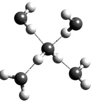
Figure 1.1 A four-coordinated water molecule showing the classic tetrahedral arrangement of the first-neighbor environment of a water molecule hydrogen-
binding to four neighbors. The hydrogen atom attached to a relatively electronegative atom is a hydrogen bond donor. The electronegative atom, such as the oxygen atom, is a hydrogen bond acceptor. Based on the transfer of electron density, the central molecule „donates‟ two hydrogen bonds to its two lower neighbors and „accepts‟ a
hydrogen bond from each of its two upper neighbors [6]. ... 2 Figure 1.2 The phase diagram of ice [6]. ... 3 Figure 1.3 How water behaves at different hydrophobic elements: extended surfaces,
biomolecules, and SWNTs [29]. ... 5 Figure 1.4 Illustration of water adsorption in SWNTs, in microporous activated carbons derived from PEEK, and on the surface of biomolecules. ... 6 Figure 1.5 The IUPAC classification of adsorption isotherms for gas-solid
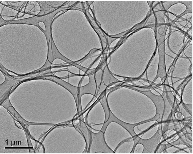
equilibria [33]... 11 Figure 1.6 In situ water loading system for NMR spectrometer at 34 MHz. ... 18 Figure 1.7 In situ gas and vapor loading system for NMR spectrometer at 300 MHz. ... 19 Figure 2.1 The TEM image of SWNTs. It shows that the samples in the current
experiment are relatively long (>1µm) and devoid of magnetic particles. ... 24 Figure 2.2 1H NMR spectrum of ethane adsorbed in SWNTs. The spectrum is taken
at 108 kPa and at room temperature. The dashed lines are Lorentzian fits. The sharp peak (blue) and the broad peak (red) are assigned to the ethane outside and inside the
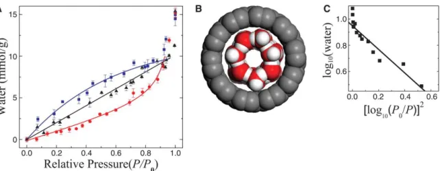
SWNTs, respectively. This shows that the SWCNTs are open for adsorption. ... 25 Figure 2.3 Water adsorption isotherms in SWNTs. (A) Three isotherms at 8.0°C
(squares), 18.4°C (triangles), and 22.1°C (circles) are shown (The uncertainty of T is ±0.3°C). The lines are guides to the eye. The vertical error bars are shown when they are larger than the size of the symbols and the pressure uncertainty is less than 1% of
xv
identified. The corresponding T2 values are shorter than the theoretically expected values for reasons explained in the text. The correlation times at these two temperatures become the same at P/P0=1 (26 ns). ... 31 Figure 3.1 Illustrations of (a) capillary phenomena at macroscopic scale and (b)
capillary condensation at microscopic scale. ... 37 Figure 3.2Water adsorption isotherms in three microporous activated carbons derived from PEEK with different amount of burn-offs at room temperature. Isotherms are fitted to Eq. (3.1), with fitting parameters shown in Table I. The inset shows the water spin-lattice relaxation time at different relative pressure. ... 38 Figure 3.3 (a)1H NMR spectra of H2 at the pressure of 100 atm with different amounts of preadsorbed D2O in the sample with 35 wt% burn-off. (b) The binary isotherms with H2 and D2O based on the peak intensity of upfield peak in H2 spectra. Water adsorption in the same sample is duplicated on the plane of H2 pressure of 100 atm. ... 40 Figure 3.4 Pore size distribution determined from water adsorption isotherms and from the differential pore volume determined from N2 adsorption at 77k in Ref [17]. The data are converted from the isotherms shown in Figure 3.2. The dashed lines are fitted to Eq. (3.2). The inset shows the correlation of pore size d with the condensation
pressure characterized by A. The data obtained from three samples give a straight line. ... 47 Figure 4.1 (a) A van der Waals representation of a lysozyme molecule colored with a
hydrophobic scale: white = hydrophobic, red (dark gray) = hydrophilic, orange (gray) = positive or negative charge. (b) A lattice model of protein hydration. The white chain represents a lysozyme molecule occupying x lattice cells. The blue (gray) spheres are hydration water, each of which occupies one lattice cell. Their locations are obtained from hydration water of less than 0.34 nm away from the protein in molecular dynamics simulations shown in Section 4.3.6. ... 51 Figure 4.2 (a)NMR spectra of lysozyme powder before (open circle) and after
pumping (filled circle). (b) The sharp NMR peak corresponding to the hydration water of protein as the temperature decreases from 4°C to -34°C. The initial hydration level is
h~0.21 at 4°C. The inset shows the hydration levels estimated from the integrated
intensities of such sharp peaks. ... 55 Figure 4.3 Water sorption isotherms in lysozyme powder from 18°C to 2°C. The
isotherms at high relative pressure are fitted as the implicit form of Eq. (4.2) with parameters shown in Table 4.1. The inset plots 0
(el)
N versus temperature. ... 56 Figure 4.4 Plots of [ln(P/P0)-lnv1-v2]/v22 versus [(v2-1/3-1)(5/3v2-1/3-1)/v22] for the
isotherms data following Eq. (4.2). The plots show a linear portion when [ln(P/P0)-lnv
1-v2]/v22>0.6. The fitting parameters are shown in Table 4.1 for =1. The inset shows the comparison of the temperature dependence of the elastic modulus (red square) derived from isotherms in this study, with the Young‟s modulus of hydrated lysozyme (red
xvi
Figure 4.5 A ribbon representation of lysozyme structure from an averaged structure from the last 5 ns of 11 ns NPT simulations at 18°C and P/P0 = 1. The residues with elevated fluctuations and correlated motions by hydration water are highlighted in red (dark gray, residues 44-53) and in yellow (light gray, residues 59-81). The residues with low fluctuations in the β-domain are shown in orange (gray, residues 54-58). Residues that are essential for the completion of the enzymatic reaction (Glu35 and Asp52) are shown in an atomic representation. The rest of the residues are shown in
a narrow ribbon representation. ... 69 Figure 4.6 All-mode correlation plots of hen egg white lysozyme from normal mode
analysis using the Gaussian network model. The NPT simulations are under comparable conditions to the experiments at relative vapor pressure of P/P0=0.6 (Nhydration =124)
(a) and P/P0=1 (Nhydration =360) (b), and the temperature of 18C. Averaged structures
from the last 5 ns of 11-ns MD simulations were used for the GNM analyses. Cross correlation of motion is color-coded using the color (gray) scale to the right. The most profound increases in diagonal intensities are from residues 44-53 (upper-left dashed squares and the red region in Figure 4.5) and residues 59-81 (lower-right dashed squares and the yellow region in Figure 4.5). The corresponding increases in off-
diagonal intensities between these two residue groups are labeled by rectangles. ... 70 Figure 5.1 (a) Structure of the heme group with an iron in the center. (b) Secondary
structures and oxygen binding sites of hemoglobin (PDB: 1GZX) in a ribbon
representation. The heme groups are highlighted with a CPK representation. ... 74 Figure 5.2 Different oxidization states of hemoglobin. ... 75 Figure 5.3 Temperature-dependent water sorption isotherms in hemoglobin. The
xvii
Figure 6.3 A diagram showing the logarithm of the anesthetizing partial pressure of non-hydrogen-bonding anesthetic agents plotted against the equilibrium partial
pressure of their hydrate crystals [18]. ... 94 Figure 6.4 The structure of the hydrate crystals of small molecules, such as xenon. ... 95 Figure 6.5 Gas chromatographic partition analysis of isoflurane equilibrium binding
to BSA at 22C, pH 7.2, and a concentration of 28 mg/mL. ... 96 Figure 6.6 Most voltage-gated ion channels are relatively insensitive to general
anesthetics. general anesthesia in humans (●), as measured by the lack of a
purposeful response to a surgical incision, occurs at concentrations of halothane 4 to 30 times lower than the EC50 concentrations needed to half-inhibit peak currents through L-type Ca2+ channels (○) from clonal pituitary cells, Na+ channels (□) from the squid giant axon, or delayed rectifier K+ channels () from the squid giant
axon [5]. ... 97 Figure 6.7 (a) Identity of general anesthetic concentrations needed to anesthetize
whole animals and to inhibit luciferase activity by 50%, for a diverse range of simple anesthetics over a 100,000-fold range of potencies. The line is the line of identity [24]. (b) Clinically relevant concentrations of halothane potentiate responses to low levels of GABA (3 M) in dissociated rat brain neurons, with 50% potentiation occurring at
0.23 mM halothane, close to the EC50 for general anesthesia (arrow) [5]. ... 98 Figure 6.8 19F NMR spectra of halothane in an empty NMR tube, in dry lysozyme
and BSA. ... 99 Figure 6.9 Adsorption isotherms of methane (117.2 K), n-butane (0.0C), neopentane
(10.0C) and SF6 (-64C) in egg albumin (2% spray frozen) shown in order of low to
xviii
LIST OF ABBREVIATIONS
NMR Nuclear Magnetic Resonance
SWNTs Single Wall Nanotubes
TGA Thermogravimetric Analyzer
PEEK Polyether Ether Ketone
BET Brunauer, Emmett, and Teller
IUPAC International Union of Pure and Applied Chemistry
EPR Electron Paramagnetic Resonance
PAS Primary Adsorption Sites
TEM Transmission Electron Microscope
VWD van der Waals
BO Burn Off
DFT Density Function Theory
HEWL Hen Egg White Lysozyme
BSA Bovine Serum Albumin
MD Molecular Dynamics
PDB Protein Data Bank
GNM Gaussian Network Model
RF Radio Frequency
FID Free Induction Decay
MAC Minimum Alveolar Concentration
CHAPTER 1
INTRODUCTION
1.1 Water: Matrix of Life
1.1.1 Bulk water
Water is the most abundant compound on Earth‟s surface and the principal constituent of all living organisms [1, 2]. It is the most essential solvent to biological processes and thus often called the “molecule of life” or “matrix of life” [3, 4]. Water is also one of the most mysterious chemical compounds, known for its anomalies such as shrinking on melting [5, 6]. The water molecule consists of an oxygen atom and two hydrogen atoms, with an average O-H bond length of 0.9572 Å and H-O-H bond angle of 104.52 [1]. Water molecules interact with each other through hydrogen bonding with a strength of 20 kJ/mol [7]. The directionality of the hydrogen bond and the maximum number of neighbors a water molecule can interact with determine most of the structural and thermodynamical properties of water.
four-2
coordinated local geometry. For instance, liquid water contains a range of ring structures including five- and fourfold ones, which are less space demanding than the sixfold ring in ice Ih as shown in Figure 1.2. The removal of the crystal constraints allows the molecules to assume a large variety of local structures, many of which occupy less volume than the crystal. As temperature increases, the hydrogen bond length increases and the variation of OOO angles also increases. This allows water to explore a denser packing than ice. From 273 K to 277 K, the increase in the OOO angle variation dominates the volume change, leading to a contraction of water volume. As temperature increases above 277 K, the normal thermal expansion mechanism takes over as the increase of hydrogen bond length dominates the volume change.
3 Figure 1.2 The phase diagram of ice [6].
1.1.2 Nanoconfined and interfacial water
The role of water in protein stability and folding was first proposed by Kauzmann [8]. He pointed out that an interaction mediated by water, the hydrophobic interaction, causes the clustering of hydrophobic units [9]. The facts that oil and water don‟t mix and tend to segregate is the consequence of the hydrophobicity, where polar and charged components „like‟ water (hydrophilic, from Greek „hydros‟ (water) and „philia‟ (love)) and apolar
components „hate‟ water (hydrophobic, from Greek „hydros‟ (water) and „phobos‟ (fear))
4
force for the biomolecule to fold into its native structure comes from the different interactions of its hydrophobic and hydrophilic components with the interfacial water.
Water certainly plays an essential role in Kauzmann‟s picture. The details of its role in protein folding, structure stability, dynamics and function remain unclear [11-15]. As the power of molecular dynamics increases, such elucidation of details becomes possible with an explicit description of each solvent molecule [16]. For instance, how could an amino acid chain find its native structure from an astronomical number of possible configurations [17, 18]? How does the water-protein interaction affect the structure and dynamics of interfacial water and proteins [15, 19-21]?
5
results at a molecular level. It is the topic of this dissertation to provide and interpret experimental results on water in nanoscopic confinement and at the interface of biomolecules.
Figure 1.3 How water behaves at different hydrophobic elements: extended surfaces, biomolecules, and SWNTs [29].
1.1.3 Dissertation outlines
6
raised whether the water at nanometer scale obeys the macroscopic Kelvin equation. In the following chapters, I start to discuss the study on the water at the interface of proteins. In CHAPTER 4, I discuss a significant decrease of hydration water in the proximity of lysozyme at temperatures below 8C. I explain this by the reduced protein flexibility and enhanced cost in elastic energy for accommodating the hydration water at lower temperature based on the modified Flory-Huggins theory. Similar effects were also observed in hemoglobin and myoglobin as shown in CHAPTER 5. The dynamics of hydration water was studied based on the NMR spin-lattice relaxation in the presence of paramagnetic centers. Based on all the above understanding of protein hydration, in CHAPTER 6 I extend our study to the role of interfacial water in mediating the protein-anesthetic interaction. I provide evidences that the apolar molecule halothane, an inhaled general anesthetic, can be adsorbed on proteins only in the presence of interfacial water.
Figure 1.4 Illustration of water adsorption in SWNTs, in microporous activated carbons derived from PEEK, and on the surface of biomolecules.
1.2 Adsorption
7
hitting a surface, the gas molecule may lose most of its kinetic energy and momentum and stay on the surface for a certain length of time before regaining enough energy to re-evaporate. This phenomenon is called adsorption. Adsorption is a fundamental process that could reveal important surface properties such as the interaction between the gas (adsorbate) and the surface (adsorbent). The existing theories of adsorption were established to relate the measured quantities with surface properties based on fundamental physical principles [31, 32].
1.2.1 Basic quantities
If n gas molecules strike a unit area of a surface per unit time and remain there for an
average time of , the adsorbed number of molecules per unit area of surface is n.
Base on the kinetic theory of gasses, the number n can be expressed as
22 (torr) 3.52 10
2 A
N p p
n
MRT MT
(1.1)
where NAis the Avogadro constant, Rthe gas constant, M the molecular weight, T the temperature, and pthe pressure in unit of torr or millimeters of mercury. n is a very large
number. For instance, at a temperature of 20C and nitrogen pressure of 760 torr, there are more than two moles of nitrogen molecules colliding with a surface within an area of 1 cm2. Such a large number generally suggests that the adsorption establishes equilibrium with surface molecules practically instantaneously [31]. In a real experiment, it always requires some time to reach adsorption equilibrium. Such a delay is caused by the transportation of molecules that are bought from distant locations to the adsorption surface.
8
perpendicular to the surface, and Q is the heat of adsorption. 0 doesn‟t depend on the time of vibration of the constituent molecules or atoms of the adsorbing surface, but is often of the same order of magnitude, namely, 1012 ~ 1014 s.
1.2.2 Langmuir isotherm
Langmuir developed a simple picture of adsorption, namely a unimolecular layer of adsorbed molecules. He assumed that the heat of adsorption is identical for every molecule that collides with a bare surface and there is no interaction between gas molecules, and that every molecule colliding with a molecule already adsorbed on the surface returns to the gas phase. This simple assumption establishes an expression for the number of adsorbed molecules: 0 1 n
(1.2)
where 0is the number of molecules in a completely filled unimolecular layer on the surface. This is equivalent to
0 0 n n (1.3) or 0 0 0 /
1 / 1
n kp n kp
(1.4)
where I have already used Eq. (1.1) with
0 0 2
A n N k p MRT
(1.5)
9
The Langmuir isotherm could also be derived from a pure statistical mechanics point of view. Unimolecular layer adsorption is equivalent to finding the number of molecules that occupy sites with energy of on the surface, where the free gas has an energy of
0
. The partition function of one particle is
0
0
0 !
, , exp
! !
Q T
(1.6)
where
3/22 / 2 p kT MkT
. The partition function becomes
0
0
0
0
exp 1 exp
(1.7)The number of molecules adsorbed on the surface is given by
0 0 exp 1 ln 1 exp (1.8)
This is identical to Eq. (1.4).
1.2.3 Multimolecular adsorption and Brunauer-Emmett-Teller isotherm
There are scenarios that suggest the interaction between gas molecules can not be negligible. When a gas molecule collides with an adsorbed molecule on the surface, there is possibility that the gas molecule is adsorbed on top of an already adsorbed molecule. This is called multimolecular adsorption. I denote the fraction of the surface covered with unimolecular thickness as 1, the fraction with thickness of two molecules is 2, etc. The total number of molecules is
0 1 0 2 0 3 0 0
1 2 3 i i i i i i
10
The number of molecules striking the bare surface, 0
1 1
i
i i
n n
, must equal to the number of molecules that evaporate from fraction 1, which is 0 1/ . For the rest of the layers above, the time of adsorption, 1, is different from that for the first layer, . Here I assumed 1is identical for all layers. Continuing the argument for all thickness, I get0 1 0
0 1 1
i=1 i>1 i i n n (1.10)
The total number of molecules adsorbed on the surface is
1 0
0 0 0
1 1 1 0 1 1
i
i i
i
i i
n k x
i i
x x kx
(1.11)where 1 1
0 0
/ 2
n N
x p p q
MRT
,and k / 1, or
0 /
1 1 /
kp
q p k p q
(1.12)
This is the basic form of the Brunauer-Emmett-Teller (BET) isotherm.
1.2.4 Classification of isotherms
11
Figure 1.5 The IUPAC classification of adsorption isotherms for gas-solid equilibria [33].
1.2.5 Uniqueness of water adsorption
12
pore size, similar to what the Kelvin equation describes. This raises the question whether theories for the bulk phase, like the Kelvin equation, remain valid at the nanoscale. From CHAPTER 4 to CHAPTER 6, I will discuss results for water adsorption in biomolecules. At low temperature, there is a significant decrease of hydration water at high relative vapor pressure. This can not be explained by the surface adsorption picture. A solution picture based on the Flory-Huggins theory and a term originating from the elastic energy has to be introduced to account for the observed temperature dependence. The adsorption of anesthetic gas in dry and wet proteins also demonstrates behaviors beyond the surface adsorption model.
1.3 Nuclear Magnetic Resonance
13
and the interaction between adsorbates and adsorbents. It is therefore useful to review some of the basic concepts of NMR prior to its application in measuring adsorption isotherms.
Table 1.1 Gyromagnetic ratio of nuclei used in NMR and electron used in EPR.
Nucleus Spin Natural Abundance (%) 10 rad s
6 -1 T-1
/ 2 MHz T
-1
1H 1/2 99.9885 267.513 42.576
3
He 1/2 0.00014 41.065 6.536
7
Li 3/2 92.410 103.962 16.546
13
C 1/2 1.07 67.262 10.705
19
F 1/2 100 251.662 40.053
129
Xe 3/2 21.180 -73.997 -11.777
electron 1/2 100 -1.76×10⁵ -2.8×10⁴
1.3.1 Magnetization
Many atomic nuclei have non-zero spin angular momentum I and a dipolar magnetic moment I collinear with it, where is gyromagnetic ratio. When placed in a magnetic field H0in zdirection, nuclear spins in the ensemble quantize along the magnetic field with a quantum number of Iz m , leading to different magnetic energy
0 0
m
E H mH . The populations Pm of the energy levels are proportional to
0
14
0 0 exp / exp / I m I I m Im mH kT
M N mH kT
(1.13)With high temperature approximation, H0/kT 1, the net magnetization reduces to
2 2
0 1 3
N I I
M H
kT
(1.14)
Table 1.1 shows the gyromagnetic ratio of several important nuclei that are commonly used in NMR. The gyromagnetic ratio of the electron is much larger than that of nuclei. The basic principles used in NMR are also applied in EPR [40]. When subject to external perturbation, such as an oscillating magnetic field at the Larmor frequency, H0, perpendicular to the static field, the net magnetization will start processing like a single spin. The change of magnetization will be determined by its Hamiltonian.
1.3.2 Interactions
The Hamiltonian of a single spin in an alternating magnetic field in terms of the amplitude 0
x
H is
0 cos
o z x x
H I H I t
(1.15)
For an ensemble of nuclear spins, there are many other interactions need to be included in the Hamiltonian. The interaction between two magnetic moments 1 1 I1and 2 2 I2in classical electrodynamics gives the expression of the quantum mechanical Hamiltonian for dipolar interaction [40]
1
2
1 2 3 5 3 d r r
r r (1.16)
15
Nuclear spins could also interact with electrons through magnetic interactions. For instance, the chemical shift originates from the orbital motion of electrons. The orbital motion of electrons changes in response to the external field, and thus alters the magnetic field at the nuclear spin. Such a change in local magnetic field is expressed in terms of resonance frequency
H0 H
H0
1
(1.17)
where is independent of H0. When the nucleus and electron are far apart, they could interact through the dipolar interaction
3 5
3 e n
e n
en
r r
r r (1.18)
For the s-state of electrons, the electron wave function is nonzero at the nucleus. This hyperfine interaction has Hamiltonian
2 8
3
hf e n I S r (1.19)
where I and
S
are the nuclear and electron spin respectively, and
r is the electron density at the nucleus. The nuclear-electron interaction is essential in the understanding of the relaxation mechanism in myoglobin and hemoglobin, where unpaired electrons are present in the molecule.1.3.3 Relaxation
16
2 2 0 1 x x x y y y z z z dM M dt T dM M dt TdM M M
dt T M H M H M H (1.20)
After a perturbation such as a RF pulse at the resonant frequency, Mhas been moved away from its thermal equilibrium value M0. In the absence of external perturbation, the net magnetization tends to move towardsM0. In the longitudinal direction, any change of Mzis associated with energy transfer from the nuclear spin to its surroundings, therefore the time constant T1 is called the spin-lattice relaxation time. On the other hand, in the transverse plane, T2 characterizes the time needed for spins lose their coherence. No energy is transferred during the spin-spin relaxation process.
In liquids and gases, molecules are experiencing constant rotational tumbling and relative translational motion. Migrations of atoms or groups of atoms from one molecule to another are common in the chemical exchange process. If the interaction between nuclear spins depends on their relative distance and direction, such as the dipolar interaction, these motions provide one of the relaxation mechanisms. The relaxation times for like spins are given by [39]
1 2
4 2
1
0 1 2
4 2
2
1 3
1 2
2
1 3 15 3
1 0 2
8 4 8
I I
I I
I I J J
T
I I J J J
T (1.21)
17
0
6 2 2
1
6 2 2
2
6 2 2
1 24 15 1 1 4 15 1 1 16 15 1 J b J b J b (1.22)
where
b
is the distance between two spins, is the Larmor period, and is the correlation time. These lead to these expressions for relaxation times:4 2
6 2 2 2 2
1 0 0
4 2
6 2 2 2 2
2 0 0
1 3 4
10 1 1 4
1 3 5 2
3
20 1 1 4
T b T b (1.23)
1.4 Experimental Setup
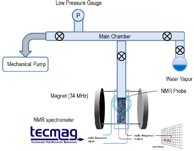
Several NMR spectrometers, at 1H NMR frequency of 34 MHz, 200 MHz, and 300 MHz, are available for in situ gas and water loading experiments in our lab. The schematics of such adsorption apparatus are shown in Figure 1.6 and Figure 1.7. The basic components are a vacuum chamber connected to a mechanical pump, a pressure gauge, the NMR sample tube, and the source of water vapor or gas. Such a vacuum chamber can be made from glass for pressure lower than 1 atm, or from stainless steel for high pressure experiments.
18
With such an in situ gas loading system attached to the NMR spectrometer, adsorption could be studied with isotherms measured by NMR on a serious of adsorbates such as water, hydrogen gas, methane and natural gas, and many other gases containing nuclear spins, such as inhaled general anesthetics.
19
20
1.5 References
[1] D. S. Eisenberg, and W. Kauzmann, The structure and properties of water
(Clarendon Press; Oxford University Press, New York; Oxford 2005).
[2] F. Franks, Water, a comprehensive treatise (Plenum Press, New York, 1972). [3] F. Franks, Water: a matrix of life (Royal Society of Chemistry, Cambridge, 2000). [4] P. Ball, Life's matrix : a biography of water (Farrar, Straus, and Giroux, New York, 2000).
[5] M. Chaplin, http://www.lsbu.ac.uk/water/index.html
[6] J. L. Finney, Philos. Trans. R. Soc. Lond., B, Biol. Sci. 359, 1145 (2004).
[7] K. A. Dill, Molecular driving forces : statistical thermodynamics in chemistry and biology (Garland Science, New York, 2003).
[8] W. Kauzmann, Adv. Protein. Chem. 14, 1 (1959). [9] D. Chandler, Nature 437, 640 (2005).
[10] D. Chandler, Nature 417, 491 (2002).
[11] H. Frauenfelder, Physics of proteins: an introduction to biological physics and molecular biophysics (Springer, New York ;London, 2010).
[12] H. Frauenfelder et al., Proc. Natl. Acad. Sci. USA 106, 5129 (2009). [13] H. Frauenfelder et al., Proc. Natl. Acad. Sci. USA 103, 15469 (2006).
[14] H. Frauenfelder, P. W. Fenimore, and B. H. McMahon, Biophys. Chem. 98, 35 (2002).
[15] R. M. Daniel et al., Annu. Rev. Biophys. Biomol. Struct. 32, 69 (2003). [16] G. A. Papoian et al., Proc. Natl. Acad. Sci. USA 101, 3352 (2004). [17] K. A. Dill, and H. S. Chan, Nat. Struct. Biol. 4, 10 (1997).
[18] Y. Levy, and J. N. Onuchic, Annu. Rev. Biophys. Biomol. Struct. 35, 389 (2006). [19] R. G. Bryant, Annu. Rev. Biophys. Biomol. Struct. 25, 29 (1996).
21 [22] D. A. Doyle et al., Science 280, 69 (1998).
[23] J. L. England, D. Lucent, and V. S. Pande, J. Am. Chem. Soc. 130, 11838 (2008). [24] J. C. Rasaiah, S. Garde, and G. Hummer, Annu. Rev. Phys. Chem. 59, 713 (2008). [25] S. Vaitheeswaran et al., Proc. Natl. Acad. Sci. USA 101, 17002 (2004).
[26] G. Hummer, J. C. Rasaiah, and J. P. Noworyta, Nature 414, 188 (2001). [27] D. M. Huang, and D. Chandler, Proc. Natl. Acad. Sci. USA 97, 8324 (2000). [28] K. Lum, D. Chandler, and J. D. Weeks, J. Phys. Chem. B 103, 4570 (1999). [29] S. Granick, and S. C. Bae, Science 322, 1477 (2008).
[30] H. Acharya et al., Faraday Discuss. 146, 353 (2010).
[31] J. H. de Boer, The dynamical character of adsorption (Clarendon, Oxford, 1968). [32] S. J. Gregg, and K. S. W. Sing, Adsorption, Surface Area, and Porosity (Academic Press, London, New York, 1982), pp. 228.
[33] J. Rouquerol et al., Pure Appl. Chem. 66, 1739 (1994). [34] R. J. Anderson et al., J. Am. Chem. Soc. 132, 8618 (2010). [35] A. Kleinhammes et al., Phys. Rev. B 68, 075418 (2003). [36] H. J. Wang et al., Science 322, 80 (2008).
[37] H. J. Wang, A. Kleinhammes, and Y. Wu, (in preparation). [38] H. J. Wang et al., Phys. Rev. E 83, 031924 (2011).
[39] A. Abragam, The Principles of Nuclear Magnetism (Clarendon Press, Oxford, 1961). [40] C. P. Slichter, Principles of magnetic resonance (Springer-Verlag, Berlin ;New York, 1990).
CHAPTER 2
TEMPERATURE-INDUCED HYDROPHOBIC-HYDROPHILIC
TRANSITION OBSERVED BY WATER ADSORPTION
2.1 Introduction
Water in the immediate vicinity of hydrophobic surfaces plays a crucial role in various important phenomena such as the folding and activity of proteins [1, 2], but experimental signatures of these water layers have been proven difficult to obtain. One possibility is that the structures and dynamics of nanoconfined interfacial water could possess distinctive temperature dependences (analogous perhaps to the anomalous density maximum manifested by bulk water at 4°C). A temperature dependence in the properties of interfacial water could be important for various processes, such as the cold denaturation of proteins [2].
23
adsorption isotherms in activated carbon [12], were likely too high to reveal the intrinsic adsorption properties of SWNTs. Water adsorption isotherms in SWNTs depend on both the interaction with the surface and the structure of the adsorbed water, which could depend on temperature. Here I report a hydrophobic-hydrophilic transition upon cooling from 22.1°C to 8.0°C, revealed by water adsorption isotherms on the inside surfaces of low-defect SWNTs. Strong evidence is provided for the formation of monolayer water inside SWNTs at 8.0°C. Nuclear magnetic resonance (NMR) studies show the dynamics of the reorientation of nanoconfined water molecules to be much slower than in bulk water. In addition to various important biological processes, this new phenomenon could also shed light on the intrinsic adsorption mechanism of water in nanoporous carbon [12, 13].
2.2 Experiments
24
Figure 2.1 The TEM image of SWNTs. It shows that the samples in the current experiment are relatively long (>1µm) and devoid of magnetic particles.
25
kPa); no bulk water is condensed outside the SWNTs below the saturated vapor pressure (P0). Furthermore, water molecules are too large to access the interstitial sites of 1.4 nm diameter SWNTs bundles [15]. Thus, the 1H NMR signal is associated predominantly with the water adsorbed inside the SWNTs [11]. The water content is calibrated by the ethane 1H NMR spectra as described in details elsewhere [10, 15].
26
2.3 Results and Discussion
2.3.1 Water adsorption isotherms in SWNTs
The amount of adsorbed water measured by 1H NMR versus the relative pressure
P/P0 at 8.0°C, 18.4°C, and 22.1°C is shown in Figure 2.3A. All three isotherms differ substantially from the S-shaped type V isotherm as observed in activated carbon and defective cut SWNTs, where adsorption increases slowly at low relative pressure but increases sharply above P/P0=0.5, quickly reaching the level of saturation [10]. Such an S-shaped adsorption isotherm in activated carbon is often attributed to PAS [12]. Figure 2.3A shows that this ubiquitous sharp increase in the isotherms of activated carbon near P/P0=0.5 is absent in low-defect SWNTs. The isotherm at 22.1°C exhibits the concave pattern of a type III isotherm, typical for clean hydrophobic surfaces with surface-water interactions weaker than water-water interactions [18]. Interestingly, the isotherm at 8.0°C exhibits a convex pattern, a type II isotherm such as that observed on hydrophilic surfaces [19]. The isotherm at 18.4°C shows a linear pattern, which is a transitional pattern between the hydrophilic isotherm at 8.0°C and the hydrophobic isotherm at 22.1°C.
27
Figure 2.3 Water adsorption isotherms in SWNTs. (A) Three isotherms at 8.0°C (squares), 18.4°C (triangles), and 22.1°C (circles) are shown (The uncertainty of T is ±0.3°C). The lines are guides to the eye. The vertical error bars are shown when they are larger than the size of the symbols and the pressure uncertainty is less than 1% of P0. (B) An illustration of monolayer water in SWNTs with a diameter of 1.36 nm. Monolayer adsorption forms a tube-like structure at 8.0°C under the constraint of the SWNTs. (C) A logarithmic plot of water content versus [log10(P0/P)]2 for the isotherm at 8.0°C, following the Dubbin-Radushkevitch-Kaganer equation.
2.3.2 Dubinin-Radushkevitch-Kaganer equation
More insight can be gained by analyzing the isotherm at 8.0°C with the Dubinin-Radushkevitch-Kaganer equation [18]. It describes monolayer adsorption, given by:
210 10 10 0
28
the water adsorption isotherm at 8.0°C and its upward turn at P/P00.8 are also evidences of molecular layering on the adsorbed surface [22]. This layering effect is commonly seen in liquid films (above the triple-point temperature of the bulk liquid) of simple hydrocarbons and inert gases on graphite.
2.3.3 Local excess chemical potential
Water adsorption is a process of balancing the chemical potential of the confined water and the vapor. When water is confined in SWNTs, the energy loss from the breaking of hydrogen bonding (~20 kJ/mol) will not be completely compensated by the van der Waals interaction (<15 kJ/mol) [23]. However, the local excess chemical potential is dominated not by the average binding energy, but by the low binding energy part, as determined by:
exp(ex) exp(u)
pbind( ) exp(u u du) (2.2) where = 1/kBT, pbind(u) is the probability distribution of binding energy u (u <0), and ex is the local excess chemical potential defined by the difference of chemical potential of water and that of an ideal gas under the same conditions [3].29
an unfavorable condition for adsorption. Thus, much less water was adsorbed in SWNTs at 22.1°C than at 8.0°C.
2.3.4 NMR relaxation and molecular reorientation
To investigate the dynamics of adsorbed water molecules, the correlation time of molecular motion was estimated with 1H spin-lattice relaxation time (T1) and the transverse relaxation time (T2). The 1H T1 in water is determined by interaction fluctuations induced by molecular motions characterized by a correlation time τ. Assuming that the intramolecular proton-proton dipolar interaction of water molecules dominates the relaxation process , T1 is given by [26]:
4 2
6 2 2 2 2
1 0 0
1 3 4
10 1 1 4
T r
(2.3)
where γ is the gyromagnetic ratio of the proton, 2πħ is the Planck constant, r is the distance between the two hydrogen atoms in a water molecule, and ω0/2π is the Larmor frequency (34 MHz at 0.8 T). A quantitative relation between T2 and τ can also be established [27]:
4 2
6 2 2 2 2
2 0 0
1 3 5 2
3
20 1 1 4
T r
(2.4)
Figure 2.4C plots the theoretical values of T1 and T2 versus τ. The measured T1 values versus pressure at 8.0°C and 18.4°C are shown in Figure 2.4A. The T1 at 8.0°C is shorter than that at 18.4°C at the same relative pressure until the saturated pressure is reached, where
30
Similarly, at 8.0°C, T2 (Figure 2.4B) increases slowly with pressure up to P/P0=1.0 whereas at 18.4°C, T2 increases very slowly below P/P0=0.8 but increases sharply above
P/P0=0.8. T2 is longer at 8.0°C than at 18.4°C at low relative pressure and becomes comparable at saturated pressure. This measurement reveals that T2 is much shorter than T1. Also, T2 increases while T1 decreases with either increasing relative pressure or decreasing temperature. Thus, the measured T1 values are situated to the right of the T1 minimum (slow-motion limit) as illustrated in Figure 2.4C by the data at P/P0=0.75. The measured T2 values at P/P0=0.75 are shorter than theoretical predictions, as plotted in Figure 2.4C. The theoretical prediction of T2 considers only the intramolecular dipolar interaction and underestimates the relaxation rate 1/T2, which also depends on the intermolecular dipolar interactions. The molecular motions under confinement are anisotropic and the intermolecular dipolar interaction cannot be easily be averaged to zero [28, 29].
31
Figure 2.4 Relaxation time of confined water. The measured T1 (A) and T2 (B) values versus relative pressure at 8.0°C (squares) and 18.4°C (triangles) are shown. The theoretical values of T1 and T2 based on the intramolecular dipolar interaction are shown in (C). Based on the measured T1 values at P/P0=0.75, 7 ms at 18.4°C and 3 ms at 8.0°C, the corresponding correlation times of 132 and 46 ns, respectively, are identified. The corresponding T2 values are shorter than the theoretically expected values for reasons explained in the text. The correlation times at these two temperatures become the same at P/P0=1 (26 ns).
Because the intramolecular dipolar interaction dominates the spin-lattice relaxation, the long correlation time τ suggests there is a substantial slowdown in molecular reorientation. The slowdown of certain dynamics of water in proximity to small hydrophobic groups has been shown previously [30]. Here I show a similar slowdown of water reorientation in proximity to an extended nonpolar surface.
2.4 Conclusion
32
free energy. When such an ordered structure is weakened at higher temperature, the distribution of the binding energy broadens, making adsorption unfavorable.
The hydrophobicity should not be considered as an absolute property of a surface under nanoconfinement without considering the structure of interfacial water. The correlation time of water reorientation in SWNTs is determined to be on the order of 10 to 100 nanoseconds. This result shows that the dynamics of water reorientation is hindered compared to bulk water, consistent with the dynamics of water molecules in proximity to small hydrophobic groups [30]. Confined and interfacial water are prevalent in biological systems, such as the water in ion channels and in proximity to proteins. The affinity change due to the temperature-induced structural change of water could be relevant to various phenomena including in biological systems, such as the cold denaturation of proteins [2].
2.5 Acknowledgements
33
2.6 References
[1] D. Chandler, Nature 437, 640 (2005).
[2] C. J. Tsai, J. V. Maizel, and R. Nussinov, Crit. Rev. Biochem. Mol. Biol. 37, 55 (2002).
[3] G. Hummer, J. C. Rasaiah, and J. P. Noworyta, Nature 414, 188 (2001). [4] K. Koga et al., Physica A 314, 462 (2002).
[5] R. J. Mashl et al., Nano Lett. 3, 589 (2003).
[6] A. I. Kolesnikov et al., Phys. Rev. Lett. 93, 035503 (2004). [7] Y. Maniwa et al., Chem. Phys. Lett. 401, 534 (2005). [8] A. Striolo et al., Adsorption 11, 397 (2005).
[9] J. K. Holt et al., Science 312, 1034 (2006).
[10] S. H. Mao, A. Kleinhammes, and Y. Wu, Chem. Phys. Lett. 421, 513 (2006). [11] M. Lagi et al., J. Phys. Chem. B 112, 1571 (2008).
[12] R. S. Vartapetyan, and A. M. Voloshchuk, Usp. Khim. 64, 1055 (1995). [13] T. Ohba, H. Kanoh, and K. Kaneko, J. Am. Chem. Soc. 126, 1560 (2004). [14] X. P. Tang et al., Science 288, 492 (2000).
[15] A. Kleinhammes et al., Phys. Rev. B 68, 075418 (2003). [16] H. Z. Geng et al., Chem. Phys. Lett. 399, 109 (2004). [17] Y. Maniwa et al., Nat. Mater. 6, 135 (2007).
[18] S. J. Gregg, and K. S. W. Sing, Adsorption, Surface Area, and Porosity (Academic Press, London, New York, 1982), pp. 228.
[19] J. Pires et al., Adsorption 9, 303 (2003).
[20] T. R. Jensen et al., Phys. Rev. Lett. 90, 086101 (2003). [21] O. Byl et al., J. Am. Chem. Soc. 128, 12090 (2006).
34
[24] T. Kurita, S. Okada, and A. Oshiyama, Phys. Rev. B 75, 205424 (2007). [25] D. Takaiwa et al., Proc. Natl. Acad. Sci. USA 105, 39 (2008).
[26] A. Abragam, The Principles of Nuclear Magnetism (Clarendon Press, Oxford, 1961). [27] R. Kubo, and K. Tomita, J. Physical Soc. Japan 9, 888 (1954).
[28] J. P. Korb, S. Xu, and J. Jonas, J. Chem. Phys. 98, 2411 (1993). [29] J. Baugh et al., Science 294, 1505 (2001).
CHAPTER 3
BULK-LIKE PROPERTIES OF WATER IN NANOSCOPIC
CONFINEMENT
3.1 Introduction
In CHAPTER 2, I discussed the unique properties of water confined in SWNTs of 1.4 nm in diameter [1]. SWNTs represent one kind of nanoscopic tubular structures for nanoconfined water [2, 3]. Both the geometrical constraints imposed by SWNTs and the surface chemistry of the confining surfaces may affect the structure, dynamics, and thermodynamics of the nanoconfined water [4-7]. For instance, at room temperature, water can assume a layered structure between extended hydrophobic plates with a separation of ~1 nm [8]. It is an obvious question to ask how nanoconfined water behaves in different geometries and different surface chemistry. In this chapter, I will discuss the properties of water confined in slit-shaped pores at the nanoscale.
36
nanotubes can align the dipoles of the water molecule chains to a length of ~0.1 mm with a persistence time of ~0.1s [9]. Another example includes the capillary phenomenon, in which the height of water between two parallel hydrophilic plates dipped into water raises to a greater height than the water outside (see Figure 3.1A) [10]. The stronger solid-liquid interaction creates a curved liquid-vapor interface between the two plates. Such a curvature reduces the liquid pressure in the proximity of the liquid-vapor interface and pushes the interface higher than the water outside, with the height inversely proportional to the separation of two plates (hd1). It remains an open question whether such phenomena and theory will persist as the separation decreases from a macroscopic length to a molecular level, up to the point just before they make contact and the water is squeezed out. The key for such phenomena is that the liquid pressure (pL) is reduced at the solid-liquid-vapor interface. Such liquid pressure (pL) is equivalent to the vapor pressure (pV) at which the liquid-vapor equilibrium appears in wettable nanopores through the capillary condensation. In this chapter, I provide experimental evidence that water confined in wettable micropores demonstrates properties similar to those of bulk water, including molecular reorientation and capillary condensation.
Water in different phases is characterized by different molecular dynamics and thermodynamics. The former can be evaluated by nuclear magnetic resonance (NMR) through the spin-lattice relaxation time (T1), a characteristic time which indicates how fast the Zeeman energy of the nuclear spins can be transferred into the thermal energy. In water,
37
isotherms by NMR to obtain molecular dynamics and thermodynamics at the same time. Here, I measured water adsorption isotherms in a series of microporous activated carbons with pore sizes ranging from 1.2 to 2.4 nm using an NMR probe connected to an in situ water and gas loading system at room temperature [1, 12, 13]. During such adsorption, the T1 of water increases from ~100 ms to ~1 s, the latter of which is close to that of bulk water (~3 s). These isotherms showed signatures of capillary condensation [14]. The condensation occurs at higher vapor pressure in larger pores, following a similar relation to that described by the Kelvin equation. These results suggest that water starts behaving like bulk water when confined in pores as narrow as 1.2 nm, in terms of molecular dynamics and thermodynamics. Such a method could be extended for characterization of pore size distribution in a series of microporous materials [15].
38
0.0
0.2
0.4
0.6
0.8
1.0
0
10
20
30
40
20 wt% BO
35 wt% BO
90 wt% BO
W
ate
r (
mm
ol/
g)
Relative Pressure (
P
/
P
0)
0.4 0.6 0.8 1.0
200 400 600 800
T
1(
ms)
Relative Pressure (
P
/
P
0)
Figure 3.2 Water adsorption isotherms in three microporous activated carbons derived from PEEK with different amount of burn-offs at room temperature. Isotherms are fitted to Eq. (3.1), with fitting parameters shown in Table I. The inset shows the water spin-lattice relaxation time at different relative pressure.
3.2 Experiments
39
by a solid echo with a /2 pulse of ~4 s. The spin-relaxation time was measured by the standard saturation recovery methods. The intensities of the 1H NMR signals were calibrated with a test tube of bulk water of known volume (0.11 cm3) with corrections for Gaussian decay [11].
3.3 Results and Discussion
Figure 2 shows water adsorption isotherms in three samples, plotted as the amount of water uptake (mmol of water per gram of activated PEEK) versus the relative water vapor pressure (P/P0, where P0 is the saturation vapor pressure) at room temperature. The isotherms exhibit a similar S shape as characterized by the Type V isotherm: a small amount of water is adsorbed on the surface functional groups as the primary adsorption sites (PAS) at P/P0<0.5 followed by a steep increase at 0.5<P/P0<0.7 and a saturation in water uptake at P/P0>0.7 as a clear signature of capillary condensation [18, 19].
3.3.1 Binary adsorption isotherms of H2 and D2O
Water and high-pressure H2 adsorption isotherms suggest that the capillary condensation of water occurs in the same micropores as that of H2 does. The binary adsorption isotherms of H2 and D2O (Cambridge Isotope, purity 99.9%) in the 35 wt% burn-off sample at room temperature were measured by 1H NMR at ~4.7T (1H NMR frequency of 200 MHz). A single pulse of ~10 s (a /2 pulse) was used for excitation. The in situ gas loading system is capable of H2 pressure up to 100 atm [16]. The sample with 35 wt% burn-off was allowed to reach equilibrium with a certain vapor pressure of D2O before measuring the adsorption isotherm of H2 up to ~100 atm at room temperature. Figure 3.3(a) shows the 1
40
with increasing amounts of preadsorbed D2O. Figure 3.3(b) plots the fractional intensity of the upfield peaks,
2
H
, relative to the intensity of the peak at 100 atm with no preadsorbed
D2O, versus the pressure of H2 and the relative pressure of D2O. For comparison, the reversed water adsorption isotherm (
2
1H O versus P/P0) in the same sample is plotted on the plane corresponding to the H2 pressure of 100 atm. A good correlation between the increase of D2O and the decrease of H2 suggests D2O residues in the same pores as H2 does. The small error here could be due to error in measuring the water vapor pressure in a much larger stainless steel system.
20 10 0 -10 -20
0 torr 8 torr 10 torr 12 torr
1
H NMR Frequency (ppm)
100 atm H2 after D2O adsorption
0.0 0.2 0.4 0.6 0.8 1.0 0.0 0.2 0.4 0.6 0.8 1.0 0 20 40 60 80 100
H2 Pre ssure (atm) Relative Va por Pre ssu
re (P/P
0)
Figure 3.3 (a) 1H NMR spectra of H2 at the pressure of 100 atm with different amounts of preadsorbed D2O in the sample with 35 wt% burn-off. (b) The binary isotherms with H2 and D2O based on the peak intensity of upfield peak in H2 spectra. Water adsorption in the same sample is duplicated on the plane of H2 pressure of 100 atm.
41
water (~3s). These are very different from the case of water in SWNTs of 1.4 nm in diameter where the T1 are much shorter and depends little on the change of relative pressure [1, 12, 13]. Such long T1 has not been observed by previous NMR measurements of adsorbed water in activated carbons, where surface relaxation centers of PAS dominate the T1 [20]. This suggests the water, even confined in nanoscopic pores, could have similar molecular reorientation as bulk water, reflected by the spin lattice relaxation mechanism [11].
3.3.2 Water adsorption in activated carbons
42
increases but the PAS remains at low density. Such a low density of PAS is crucial to explore the effect of pore size on capillary condensation.
3.3.3 Mahle’s isotherm
Low water uptake at P/P0<0.5 suggests a small amount of PAS. As the vapor pressure increases, the isotherm increases within a narrow range of pressure and then bend towards high relative pressure. This is the signature of capillary condensation. It suggests that the pores are filled with water and activated carbons are wettable due to the cooperativity of water [25]. The capillary condensation occurs at a higher relative pressure in the sample with higher burn-off. Characterizations of the pore size by N2 and H2 adsorption have shown that a higher burn-off corresponds to a larger pore size of a few nanometers as listed in Table 3.1 [16, 17]. This indicates that the pore size (d) is the dominating factor in capillary condensation. The measured symmetric S-shaped isotherm represents a distribution of condensation pressures with a Lorentzian distribution. It can be fitted into the isotherms provided by Mahle as expressed in the amount of adsorbed water versus relative pressure (P/P0) via [15]:
1 / 0 1
tan tan
s
n P P A A
n
D B B
(3.1)
where n and ns are the number of adsorbed water molecules at P and P0, respectively, A and
B , expressed in units of P/P0, are related to the center and the distribution of the condensation pressures respectively, and the normalization coefficient D is given by
1 1
tan 1 / tan /
43
Table 3.1 Parameters characterizing three activated carbons derived from PEEK. A, B, and
ns/D are used to fit the water adsorption isotherms to Eq. (3.1). The pore size and BET surface area are determined in ref [16, 17].
Burn-off (wt %)
A
(P/P0)
B
(P/P0)
ns/D (mmol/g)
nsVL
(cm3/g)
d
(nm)
Surface Area (m2/g)
20 0.543±0.006 0.112±0.008 11.4±0.2 0.55 1.2 1294
35 0.592±0.005 0.080±0.006 9.3±0.2 0.47 1.4 981
90 0.775±0.003 0.067±0.004 15.3±0.3 0.79 2.4 2802
3.3.4 Pore size distribution
The relation between the center value of the condensation pressure (A) and the pore size (d) is shown in Figure 3.4 by plotting d (nm) vs. 1 / ln
P P/ 0
. A simple linear fittinggives
0
0.52 / ln / 0.38
d P P (3.2)
Such a relationship allows us to convert the water adsorption isotherms into pore size distributions via [15]
1 2 0 0 0 /1 / ln /
0.38
s L
V P P A n V
BD P P P P
d B d
(3.3)
![Figure 1.3 How water behaves at different hydrophobic elements: extended surfaces, biomolecules, and SWNTs [29]](https://thumb-us.123doks.com/thumbv2/123dok_us/8309464.2200681/23.918.155.797.250.529/figure-behaves-different-hydrophobic-elements-extended-surfaces-biomolecules.webp)

![Figure 1.5 The IUPAC classification of adsorption isotherms for gas-solid equilibria [33]](https://thumb-us.123doks.com/thumbv2/123dok_us/8309464.2200681/29.918.140.773.111.504/figure-iupac-classification-adsorption-isotherms-gas-solid-equilibria.webp)