CORTICAL SURFACE REGISTRATION AND SHAPE ANALYSIS
Ilwoo Lyu
A dissertation submitted to the faculty at the University of North Carolina at Chapel Hill in
partial fulfillment of the requirements for the degree of Doctor of Philosophy in the
Department of Computer Science in the University of North Carolina at Chapel Hill.
Chapel Hill
2017
c
2017
Ilwoo Lyu
ABSTRACT
Ilwoo Lyu: Cortical Surface Registration and Shape Analysis
(Under the direction of Martin A. Styner)
A population analysis of human cortical morphometry is critical for insights into brain
development or degeneration. Such an analysis allows for investigating sulcal and gyral
folding patterns. In general, such a population analysis requires both a well-established
cortical correspondence and a well-defined quantification of the cortical morphometry. The
highly folded and convoluted structures render a reliable and consistent population analysis
challenging. Three key challenges have been identified for such an analysis: 1) consistent
sulcal landmark extraction from the cortical surface to guide better cortical correspondence,
2) a correspondence establishment for a reliable and stable population analysis, and 3)
quantification of the cortical folding in a more reliable and biologically meaningful fashion.
The main focus of this dissertation is to develop a fully automatic pipeline that supports
a population analysis of local cortical folding changes. My proposed pipeline consists of
three novel components I developed to overcome the challenges in the population analysis:
1) automatic sulcal curve extraction for stable/reliable anatomical landmark selection, 2)
group-wise registration for establishing cortical shape correspondence across a population
with no template selection bias, and 3) quantification of local cortical folding using a novel
cortical-shape-adaptive kernel.
ACKNOWLEDEMENTS
I would like to express my gratitude to people who have supported my research and
dissertation. First, I thank my advisor Martin Styner for his patience, encouragement, and
guidance during the past five years. He was the best advisor, mentor, and friend I ever met.
Without his supports, I won’t be able to pursue my academic career. He taught me scientific
principles in the field, helped me achieve all the doctoral milestones, and inspired me with
his outstanding passion and dedication in research.
I also thank all my committee members. Stephen Pizer has been extremely eager to help
me improve my writing skills and to provide his valuable feedback to my research. I learned
his immense knowledge and understanding of the field. I thank John Gilmore for sharing
his expertise and collaboration. I also thank Marc Niethammer and Hongtu Zhu for their
insightful suggestions on my research.
I would like to thank my collaborators and fellow students in my department: Sun Hyung
Kim, Joohwi Lee, Minjeong Kim, Colin Compas, Hongzhi Wang, Yu Cao, Sangwoo Cho,
Junpyo Hong, Yaozong Gao, etc. In particular, Sun Hyung was my best collaborator. He
helped me develop ideas and shared his knowledge. Joohwi was always happy to discuss
interesting research topics. Minjeong helped me a lot especially for the first year of my study.
Colin, Hongzhi, and Yu made me feel comfortable during my entire internship at IBM.
Hyungil Seo, Hyunggu Jung, Kijung Yoon, Yong Jin Park, Sangwook Yoo, Donghoon Sagong,
Junseong Lee, Min Kim, Yukyung Choi, Geunmok Park, etc.
Lastly, and most importantly, I would like to thank my family members for their invaluable
support. My parents contributed hugely to this long journey with unconditional support
TABLE OF CONTENTS
LIST OF FIGURES
. . . xiii
LIST OF TABLES . . . xvi
Chapter 1: Introduction . . . .
1
1.1
Overview . . . .
1
1.2
Previous Work
. . . .
3
1.2.1
Sulcal Landmark Extraction . . . .
3
1.2.2
Sulcal Landmark Labeling . . . .
5
1.2.3
Cortical Surface Correspondence . . . .
6
1.2.4
Quantification of Cortical Folding . . . .
9
1.2.5
Cortical Morphological Development in Early Stage . . . .
11
1.3
Thesis Statement . . . .
12
1.4
Overview of Chapters . . . .
13
Chapter 2: Background . . . .
15
2.1
Cortical Surface Reconstruction . . . .
15
2.2
Curvature Metrics . . . .
17
2.3
Spherical Harmonic Basis Functions . . . .
19
2.5
Wavefront Propagation . . . .
23
Chapter 3: Automatic Sulcal Curve Extraction on the Cortical Surface
. .
25
3.1
Overview . . . .
25
3.2
Objective
. . . .
26
3.3
Slicing and Contour Extraction . . . .
27
3.4
Sulcal Point Detection . . . .
29
3.5
Curve Delineation . . . .
31
3.6
Materials
. . . .
34
3.7
Results . . . .
35
3.7.1
Noise Sensitivity
. . . .
36
3.7.2
Reproducibility . . . .
36
3.8
Summary
. . . .
39
Chapter 4: Robust Estimation of Surface Correspondence . . . .
41
4.1
Overview . . . .
41
4.2
Preprocessing . . . .
43
4.2.1
Automatic Sulcal Curve Labeling and Landmark Correspondence . .
43
4.2.2
Rigid Transformation for Initial Alignment on Sphere . . . .
44
4.3
Landmark-based Pair-wise Surface Correspondence . . . .
45
4.3.1
Objective
. . . .
45
4.3.2
Consistent Displacement Encoding Scheme . . . .
46
4.3.3
Initial Deformation Field . . . .
47
4.3.5
Optimal Pole Selection . . . .
50
4.4
Extension to Group-wise Surface Correspondence . . . .
51
4.4.1
Objective
. . . .
51
4.4.2
Entropy of Landmark Errors . . . .
53
4.4.3
Entropy of Multidimensional Geometric Properties
. . . .
55
4.4.4
Entropy Minimization
. . . .
55
4.4.5
Hierarchical Optimization . . . .
56
4.5
Shape Correspondence Evaluation . . . .
58
4.5.1
Average Shape Model Construction . . . .
58
4.5.2
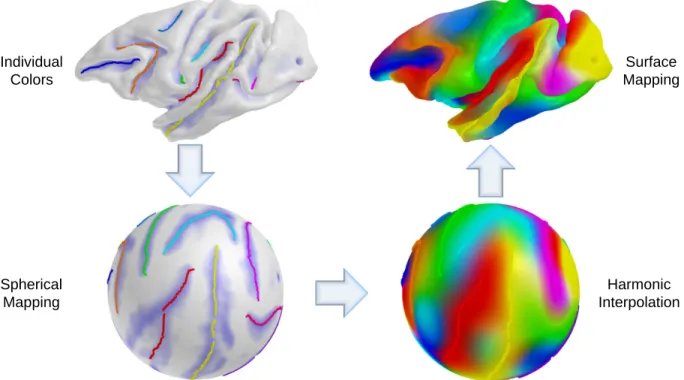
Correspondence Evaluation via Surface Coloring . . . .
58
4.6
Materials
. . . .
59
4.6.1
Macaque Cortical Dataset . . . .
59
4.6.2
IBIS Paediatric Cortical Dataset
. . . .
60
4.6.3
Non-human Primate Molar Shape Dataset . . . .
61
4.7
Results . . . .
61
4.7.1
Optimal Pole Selection . . . .
62
4.7.2
Sulcal Curve Variability . . . .
64
4.7.3
Variance over Sulcal Depth Maps and Cortical Thickness . . . .
65
4.7.4
Visual Validation on Macaque Dataset . . . .
65
4.7.5
Evaluation of Average Shape Models . . . .
66
4.7.6
Principal Component Analysis on Molar Shapes . . . .
67
Chapter 5: Sulcal Shape-Aware Quantification of Cortical Folding . . . .
71
5.1
Overview . . . .
71
5.2
Objective
. . . .
73
5.3
Outer Hull Creation and Correspondence Establishment
. . . .
74
5.4
Sulcal/Gyral Curve Extraction . . . .
75
5.5
Travel-time Map
. . . .
76
5.6
Tensor Field . . . .
77
5.6.1
Principal Propagation Direction . . . .
77
5.6.2
Principal Propagation Speed . . . .
78
5.6.3
Tensor Matrix . . . .
79
5.7
Adaptive Kernel and Local Gyrification Index . . . .
81
5.8
Materials
. . . .
82
5.8.1
IBIS Living Phantom . . . .
82
5.8.2
KIRBY Dataset . . . .
84
5.8.3
Simulated Cortical Folding . . . .
84
5.9
Results . . . .
86
5.9.1
Reproducibility . . . .
87
5.9.2
Evaluation of Simulated Cortical Folding . . . .
90
5.9.3
A Choice of Kernel Size
. . . .
91
5.10 Methodological Issues . . . .
92
5.10.1 Local Gyrification Index . . . .
92
5.10.2 Cortical-Shape-Adaptive Kernel . . . .
95
5.11 Summary
. . . .
97
Chapter 6: Cortical Morphometry and Cognitive Development in Early
Post-natal Stage . . . .
98
6.1
Overview . . . .
98
6.2
Objective
. . . .
98
6.3
The UNC Early Brain Development Studies (EBDS)
. . . .
99
6.3.1
MR Image Acquisition . . . .
99
6.3.2
Mullen Scales of Early Learning (MSEL) . . . .
100
6.3.3
Data Exclusion Criteria
. . . .
101
6.3.4
Surface Model Reconstruction and Local Gyrification Index
. . . . .
101
6.4
Linear Mixed Model for the Longitudinal Study . . . .
104
6.5
Findings of Early Morphometry and Cognitive Development . . . .
105
6.5.1
Cortical Gyrification in Early Stage . . . .
105
6.5.2
Association of Cognitive Development
. . . .
108
6.5.3
Comparisons with FreeSurfer
. . . .
109
6.6
Summary
. . . .
115
Chapter 7: Summary and Conclusion . . . 117
7.1
Summary of Contributions . . . .
117
7.2
Limitations . . . .
120
7.3
Future Work . . . .
122
7.3.1
Computational Issues . . . .
122
LIST OF FIGURES
Figure
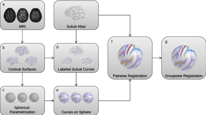
1.1
Schematic overview of the entire pipeline . . . .
14
3.1
Schematic overview of the sulcal curve extraction . . . .
27
3.2
Contour extraction . . . .
29
3.3
Sulcal point detection . . . .
30
3.4
Schematic overview of the line simplification method
. . . .
30
3.5
Candidate sulcal points . . . .
32
3.6
Endpoint detection . . . .
34
3.7
An example of estimated endpoints . . . .
35
3.8
Robustness to noise . . . .
37
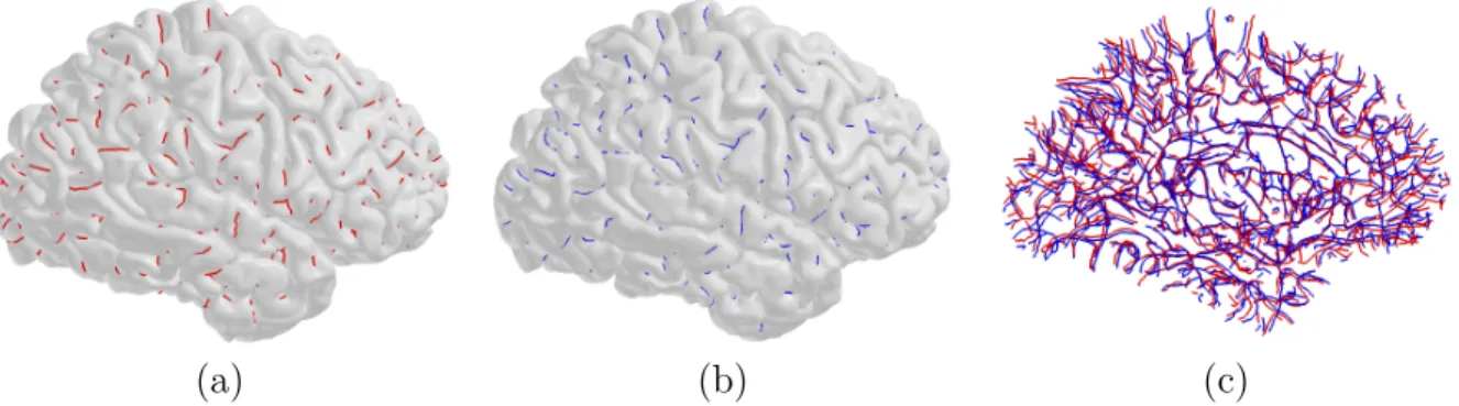
3.9
Sulcal curve extraction . . . .
38
3.10 Sulcal curve extraction errors
. . . .
39
4.1
Schematic overview of the pair-wise method . . . .
42
4.2
Schematic overview of the spectral matching . . . .
44
4.3
Landmark distribution after applying different methods . . . .
45
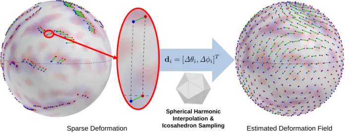
4.4
Displacement encoding and estimated deformation field . . . .
47
4.5
Artifacts in the standard polar coordinate system and reduced artifacts . . .
51
4.6
Schematic overview of the group-wise registration . . . .
52
4.7
Cortical surface coloring . . . .
59
4.9
Reconstruction errors . . . .
63
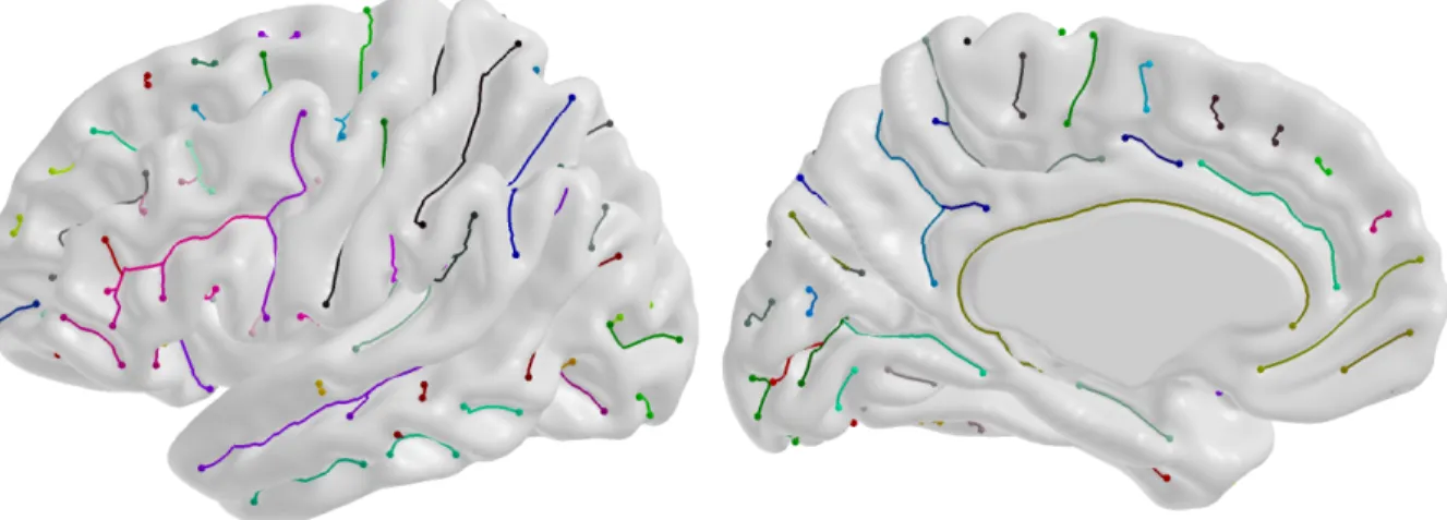
4.10 Sulcal curve alignment by different methods . . . .
64
4.11 Visual comparison of correspondence results . . . .
66
4.12 Average model reconstruction . . . .
67
4.13 Shape correspondence evaluation using reconstruction error . . . .
68
4.14 Primate fossil molar shape space . . . .
69
5.1
Schematic overview of the local gyrification index . . . .
72
5.2
Overview of the tensor field computation . . . .
73
5.3
Two different types of synthetic normalized travel-time maps . . . .
80
5.4
Kernels at an arbitrary point using different approaches . . . .
83
5.5
Simulated equally-spaced sulci . . . .
85
5.6
Reproducibility . . . .
89
5.7
Local gyrification index of the sine waved plane . . . .
91
5.8
The average local gyrification indices on the Kirby dataset . . . .
93
6.1
Pearson’s correlation coefficients of the early childhood brain dataset
. . . .
102
6.2
Correlation of gyrification index within subject . . . .
106
6.3
Age effect on cortical gyrification . . . .
107
6.4
Gender effect on cortical gyrification
. . . .
108
6.5
Gestational age effect at birth on cortical gyrification . . . .
108
6.6
Raw association with cognitive development using optimal kernel size . . . .
110
6.7
Corrected association (q <
0.05) with cognitive development . . . .
111
6.9
Comparison: association with demographic effects using large kernel size . .
113
6.10 Comparison: association with cognitive development using large kernel size .
114
6.10 Comparison: association with cognitive development using large kernel size
LIST OF TABLES
Table
4.1
Sulcal curve entropy
. . . .
64
4.2
Variances of cortical properties
. . . .
65
5.1
Average closest distance of the adaptive kernel . . . .
88
5.2
Coefficient of variation . . . .
90
CHAPTER 1: INTRODUCTION
1.1
Overview
Cortical brain morphometric measures such as cortical surface area or thickness have been
widely investigated in neuroimaging studies of brain development and degeneration. These
measures enable analyses of global or local developmental trajectories over age of anatomical
changes and their relationships with cognitive function or environment factors. In addition,
quantification of cortical folding has evolved to be an important measure for such cortical
analyses. The cortical gyrification is a dynamic process on the cortex involving surface
expansion/shrinkage as the number of neurons increases/decreases during brain growth.
However, the complete trajectory of cortical gyrification of the human brain is currently
unknown, which makes it difficult to determine an optimal measure of cortical folding as no
generic ground truth of the trajectory is available. There have been increasing attempts to
quantify gyrification in brain developmental studies and pathological disorders via a surface
expansion/shrinkage rate over the cortex of adults [2, 67, 35, 110, 56], infants [68, 62, 49], and
non-human primates [143, 144]. The main challenge comes from the nature of the cortical
shape with its highly complex and variable cortical folding patterns, which hampers the
consistency of cortical analyses. Thus, a key aspect to cortical folding analyses is to determine
where and how to measure a folding region in a consistent way.
cortical folding pattern analysis. However, the cortical folding patterns are highly complicated
and variable in both intra- and inter-subject comparisons, which makes quantification of
cortical folding challenging. Even if such quantification is well defined in a single subject,
the complexity and variability of the cortical shape yield significant challenges to a
popu-lation study without an appropriate establishment of inter-subject cortical correspondence.
Therefore, successful analyses of cortical folding patterns need to address two critical issues:
consistent anatomical/geometric landmark extraction and cortical surface correspondence.
Recently, with the advent of 3D cortical surface reconstruction, fundamental geometric
landmarks such as local curvature are easily accessible and thus commonly used in the
field of the 3D cortical surface-based analysis. Of many potential geometric properties, it
is well-known that sulcal landmarks are one of the most invariant, stable features across
cortical regions. Currently, two popular ways exist to define sulcal landmarks. The most
prevalent way is based on regional parcellation, given a shape correspondence to a template
(or reference) model. However, this approach often suffers from inaccurate boundaries due to
high sulcal variability across subjects. Another way is to extract sulcal landmarks without
utilizing any predefined template model. In this context, the main advantage comes from no
template selection bias, but the approach casts a critical question of how to define/design
sulcal landmarks.
terms of relative invariance and stability across a population. Once a set of well-described
anatomical features is obtained, the next step is to properly fuse those features into the
cortical shape correspondence establishment.
To address a cortical shape correspondence problem for a population analysis, the necessary
solutions/methods can be separated into the following sub-problem steps:
•
Anatomical/geometric landmark extraction
•
Cortical surface correspondence
•
Quantification of cortical folding patterns
•
Population analysis for a brain development study
1.2
Previous Work
1.2.1
Sulcal Landmark Extraction
As discussed already, sulcal fundic regions are known as one of the most invariant, stable
features across cortical regions and thus have been widely used as robust features for cortical
registration. Sulcal fundic region recognition has been proposed in several studies [81, 111, 71]
and employed as critical features for a cortical correspondence [28, 3, 130, 73]
through points with the maximum curvature, as discussed in [55].
Shi et al. [114] applied the Hamilton-Jacobi equation to the cortical surface to extract
sulcal curves by solving the Eikonal equation (a special form of the Hamilton-Jacobi equation).
Seong et al. [111] further proposed a more general solver that computes anisotropic geodesics.
In their method, the cortical surface is first segmented into seed regions by thresholding a
sulcal depth map, and anisotropic skeletons are then computed by solving the Hamilton-Jacobi
equation. This method requires careful parameter tuning to determine candidate points that
belong to potential sulcal curves. Moreover, since the initial seed regions for the wavefrontal
propagation are based on a sulcal depth map, the sulcal curve extraction could be quite
sensitive to the initial definition of the seed regions especially in cortical fissures with wide
sulcal fundi like the Sylvian fissure.
1.2.2
Sulcal Landmark Labeling
Many geometric methods discussed above tackled the sulcal landmark extraction problem
by exploiting geometric information such as geodesic distance or sulcal depth. However, such
a geometry-based approach generally cannot distinguish the primary cortical sulci effectively
from the secondary or tertiary sulci without an incorporation of prior knowledge about
sulcal landmarks. The recognition of the primary sulci is useful in neuroimaging applications
[97, 40], in that they are more consistent in sulcal fundic regions across different brains. For
the recognition of sulcal landmarks, one could employ cortical parcellation methods either
by analyzing structural neuroimaging data [102, 12] or by combining prior neuroanatomical
information and cortical geometry [33]. However, these parcellation-based approaches often
suffer from inaccurate boundaries of the cortical parcellation due to the high variability across
subjects.
For labeling cortical features, Sandor and Leahy [109] used a manually labeled brain
atlas. An atlas encodes neuroanatomical labeling conventions determined by knowledge
on structure-function relationships and cytoarchitectronic or receptor labeling properties of
regions. Their approach warps the atlas to an individual subject’s cortical surface in order to
inherit the labels of cortical features from the atlas. Since this method depends on an atlas
registration scheme, it requires a surface correspondence between a template and subjects
and generally suffers from a template selection bias. Similar surface-registration methods
have been reported in [135, 126, 63, 64, 124].
were then labeled based on a manually labeled training set. This approach was further
extended to detection of major cortical sulci. In such an approach, joint sulcal shape priors
between neighboring sulci were used in the learning process [115]. However, the approach
simplified the sulcus detection problem by removing sulcal curves crossing over gyral regions
and representing each sulcus as a simple curve. A watershed transform-based approach
was presented in [63, 105], in which segmented regions were manually labeled by an expert.
Learning-based techniques were also proposed in [106, 5, 132, 96] to detect and label sulci.
However, these techniques depend on specific atlas registration schemes [106, 5, 96] or suffer
from lacks of neuroanatomical conventions [132]. Graph-based learning techniques were
integrated into a public-domain system BrainVisa [107], and cortical sulci that were detected
or labeled by this system have been successfully used in many neuroimaging applications
[10, 16, 15, 27, 24].
1.2.3
Cortical Surface Correspondence
(across a population at once).
Cortical surface registration employing parametrized representations is the most prevalent
in the field. It is based on mapping the cortical surface onto a specific parametrized space.
Several mapping spaces have been proposed including planar [3], hyperbolic [130] or spherical
[123, 44] parametrizations. Spherical parametrizations are most popularly used due to their
convenience, reduced distortions and computational efficiency [125, 31, 140, 95, 108, 74]. To
reduce mapping distortions in parametrization, geometric features (e.g., local curvatures,
curvedness, shape index, etc.) have been widely employed in popular pipelines such as
Freesurfer. In recent work [69, 3, 130], sulcal landmark features were employed to reduce
such mapping distortion. Alternatively, Shi et al. [116] proposed an embedding in the
Laplace-Beltrami (LB) space that incorporates a spectral representation to reduce distortions.
While these parametrization-based methods are able to provide appropriate parametrized
representations, it is noteworthy that all such parametrizations possess significant residual
mapping distortions.
implicit deformation field.
The well-studied template-based methods establish a correspondence via a prior template
model in a pair-wise manner. Spherical mapping-based methods are most commonly used
for cortical registration. Several studies [125, 31, 140, 95] have shown successful pair-wise
registration in the spherical space to allow every subject to be aligned to a single template
model. Van Essen [136] applied a surface registration method to human and even
non-human primate subjects via spherical mapping. Lyttelton et al. [70] further proposed an
iterative registration scheme that updates the initial template model for better correspondence
establishment. Lyu et al. [73] also proposed a template-based cortical registration via
spherical harmonic decomposition of the deformation field. Unfortunately, even if individual
correspondence to the template is well developed, these pair-wise methods all possess an
inherent bias to the initial template model. The specific template may also be a
non-optimal choice for the data at hand, yielding lower sensitivity and specificity in the statistical
population analysis.
implicitly defines a deformation model without guarantee of topology preservation. In other
words, this method is likely to yield over-folding of the cortical surface. Furthermore, this
method does not provide an explicit estimation of the deformation field between subjects.
1.2.4
Quantification of Cortical Folding
It is challenging to develop a good metric of cortical folding without deep insight into the
developmental trajectory of cortical folding or the modeling of cortical gyrification. In earlier
work [142, 85], the so-called gyrification index (GI) has proposed to quantitatively measure
cortical folding in the volume space by computing a ratio of the pial
1perimeter over the outer
perimeter for each slice. This provides an easy interpretation of cortical folding by globally
capturing the amount of cortical folding in each slice. Despite its clear representation, it
comes with several shortcomings as pointed out in [110]. Particularly, it is highly likely for
this 2D measure to be biased to a cutting plane selection (e.g., sagittal plane) due to loss
of cortical spatial information that is inherently defined in 3D space. In this context, the
cortical folding of a buried deep sulcus is rarely captured in a single slice. One can use 3D
manual delineation of contours over the entire cortex to overcome such limitations, but this
is a highly time-consuming and tedious task.
More recently, approaches have shifted to a 3D surface-based analysis [17, 137], which
provides a higher potential for an appropriate cortical shape analysis. Several investigations
have also been made based on various geometric representations of cortical folding. In [35],
local mean curvatures computed over the entire cortex were employed as a surrogate local
measurement of cortical folding. In [49], local shape analyses were performed using the
so-called shape complexity index based on the shape index proposed by Koenderink and
van Doorn [51] to measure a local cortical shape change over the years. Batchelor et al. [4]
investigated several geometric properties as measures of cortical folding. Similar to the 2D
GI, local gyrification can be measured in 3D space by the area ratio between the outer hull
and the pial surface [128, 110, 122, 56, 62]. An outer hull-free gyrification index was also
proposed in [117, 77]. As such measures are defined locally, regional quantification of cortical
folding is generally obtained by computing the corresponding average within a specific region
over the cortex.
across mutiple sulci/gyri [100].
1.2.5
Cortical Morphological Development in Early Stage
Several studies have found that the human brain changes dramatically during the early
postnatal phase. Total brain volume doubles in the first year of life and reaches 80% of adult
volume by the end of the second [50, 38]. Similarly, surface area grows fastest and reaches
70% of adult values in the early postnatal period; as well, cortical thickness exhibits a rapid
thickening and reaches 97% of adult values [50, 38]. Cortical changes with respect to cortical
thickness and surface area are also correlated to cortical folding development [118, 34]. In
addition, the early postnatal phase (from neonate to 2 year) is a critical period in cognitive
development [87], e.g., the development of primary sensory processing or language. According
to [88], foster care before age 2 helped children have significantly better cognitive outcomes,
as compared to kids raised in orphanages. Thus, it is important to investigate the association
of cognitive development and brain growth in the early postnatal period. Unfortunately,
there is a lack of studies that describe brain growth trajectories particularly in the early stage
[39] and their relationship to cognitive development.
1.3
Thesis Statement
Thesis:
Template-free group-wise cortical surface correspondence can be established with
the support of anatomical/geometric sulcal landmarks. Such cortical correspondence can be
employed with a local-shape-adaptive quantification of cortical folding patterns to describe
cortical gyrification trajectories in early postnatal brain development.
The contributions of this dissertation include
1.
A novel sulcal curve extraction method
: Sulcal curves are automatically extracted from
the cortical surface in a fashion robust to surface noise. My proposed method achieves
high computational efficiency, improves robustness to noise, and high reliability in a
scan-rescan dataset as compared to a well-known existing method.
2.
A template-free group-wise cortical surface correspondence
: A population correspondence
is established and improved simultaneously in a group-wise fashion free from template
selection bias. My novel group-wise registration method allows for local cortical shape
analysis in human and non-human primate neuroimaging studies. The proposed method
achieves superior results with respect to consistency across subjects as evaluated via
quantitative and visual comparisons compared to well-known existing methods.
4.
A description of trajectories of cortical gyrification and early cognition development
:
This dissertation presents an application of my entire framework to a population study
of early cortical morphometric development in local gyrification index and cognitive
development.
5.
A publicly available software package
: The source codes of the proposed pipeline
developed in this dissertation are publicly available at
http://github.com/ilwoolyu/
.
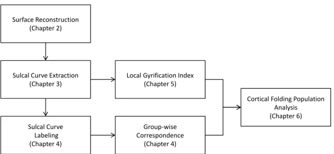
1.4
Overview of Chapters
Sulcal Curve Extraction (Chapter 3)
Local Gyrification Index (Chapter 5)
Group‐wise Correspondence
(Chapter 4) Sulcal Curve
Labeling (Chapter 4) Surface Reconstruction
(Chapter 2)
Cortical Folding Population Analysis
(Chapter 6)
CHAPTER 2: BACKGROUND
This chapter presents the background materials required for this dissertation. Section 2.1
describes an overview of popular cortical surface reconstruction methods. Section 2.2 provides
the description of geometric curvature of smooth surfaces for surface handling and geometric
property extraction throughout this dissertation. Section 2.3 briefly summarizes the spherical
harmonic basis functions employed for the deformation field representation, and Section 2.4
presents an entropy model to find an optimal geometric property agreement for group-wise
surface correspondence. At the end of this chapter, Section 2.5 presents a basic concept of
wavefront propagation over the cortical surface model, formulated by the Hamilton-Jacobi
partial differential equation (H-J PDE) for geodesic distance computation over surface models.
2.1
Cortical Surface Reconstruction
Earlier studies proposed a cortical surface model obtained along the gray matter and CSF
boundary by deforming a topologically corrected model like a sphere [78, 80]. However, such
reconstructed models generally suffered from poor representations of the narrow and deep
buried cortical folding because it is exceedingly difficult to design an energy functional that
fits the deformable model through the narrow opening of the sulci to the true cortical folding
as pointed out in [30].
More recently, approaches have sought to finding the white and gray matter boundary
to reconstruct a surface model, for example, FreeSurfer [17] or CIVET [79] pipelines. These
frameworks are quite similar in terms of two properties: 1) their surface model guarantees a
spherical topology for the white matter surface model construction. 2) the gray matter surface
is obtained by deforming the white matter surface to fit the gray matter and CSF boundary,
in which the cortical correspondence between the white and gray surfaces is inherently
established. Briefly, the overall pipeline is summarized as follows. The raw MR images are
first refined by bias field correction and intensity normalization. Then the preprocessed
images are aligned in a common space such as Talairach space for skull stripping (including
neck and eyeball) and cortical structure segmentation. The cortical tissues are segmented to
create a white matter mask by filling in the subcortical structures within the white matter.
This white matter mask is then separated into left and right hemispheres. Finally, the initial
white matter surface is obtained via a rough triangulated tessellation in FreeSurfer or via
deforming a topologically correct model in CIVET. Once the white cortical surface is obtained,
the gray cortical surface is reconstructed by deforming the white cortical surface using volume
intensity information with several geometric constraints (e.g., curvature smoothing).
been observed that the cortical surface reconstruction is also susceptible to partial volume
effects with narrow sulcal fundi (e.g., less than 1
mm) often poorly represented due to low MR
image resolution. In FreeSurfer, there are two types of topological defects as a result of such
partial volume effects in the resulting model: holes and handles are present since it creates
the surface model using a tessellation technique for the volume-wise tissue segmentation
result. In contrast, such topological defects do not exist in CIVET because a topologically
correct model is employed to fit to the white and gray boundary. However, this approach
still suffers from partial volume effects in the white and gray boundary due to the design
difficulty in energy functional. Therefore, the postprocessing is required either for topological
correction to guarantee a desirable topology [32] or for appropriate representation of narrow
cortical fundi by estimating partial volumes correctly [127].
2.2
Curvature Metrics
In differential geometry, given a point
x
on the smooth surface with the tangent (walking)
direction
T, the normal curvature at
x
quantitatively measures the amount of the surface
bend along
T
as measured by the swing of the surface normal
N
at
x. Let Ω be a smooth
surface
∈
R
3with a sufficient parametrization:
x(u, v)
∈
Ω such that
x
u
and
x
vare linearly
independent, where
u, v
∈
R
. Let
D
Tdenote the directional derivative along
T. The normal
swing at
x
along
T
is decomposed into two components: the normal curvature
κ
Tand its
geodesic torsion
τ
T:
where
T
⊥is the orthogonal direction to
T
on the tangent plane, and
N
=
x
u×
x
vkx
u×
x
vk
.
(2.2)
Similarly, the normal swing at
x
along
T
⊥is given by the normal curvature
κ
N⊥and its
geodesic torsion
τ
T⊥:
D
T⊥N
=
κ
T⊥·
T
⊥+
τ
T⊥·
T.
(2.3)
These properties are represented as a matrix form:
D
TN
D
T⊥N
=
κ
Tτ
Tτ
T⊥κ
T⊥
T
T
⊥ .
(2.4)
Call the 2
×
2 matrix
M
II. The geodesic torsion is the same regardless of the tangent direction
T, i.e.,
τ
T=
τ
T⊥. The associated eigenvalues of
M
IIare called principal curvatures that
capture the pure normal swing along the eigenvectors with no geodesic torsion. To improve
the ability of shape description, the principal curvatures (κ
1≤
κ
2) are further extended to
the following geometric properties: mean curvature
H, Gaussian curvature
K, shape index
S
[51], and curvedness
C
[51].
H
=
1
2
(κ
1+
κ
2),
K
=
κ
1·
κ
2,
S
=
−
2
π
tan
−1
κ
1+
κ
2−κ
1+
κ
2
,
C
=
2
π
log
s
(κ
21
+
κ
22)
2
.
Here is a brief description of those curvature metrics. The mean curvature
H
is the average
of the principal curvatures; it equals the average normal curvatures over all directions. This
quantification is an extrinsic measure and is equivalent to a half of the trace of
M
II. The
Gaussian curvature
K, log(det
M
II), summarizes the swings of the normal per unit area; also,
it is intrinsic in a sense of invariance to local isometries. Both
H
and
K
are invariant to
the choice of bases and to rigid transformation, whereas these measures are not invariant to
scaling. The shape index
S
and curvedness
C
were originally proposed to describe local shape
in a more intuitive way. For example, Koenderink and van Doorn [51] argued that although
spheres with different sizes intuitively have the same shape,
H
and
K
fail to describe such a
property.
S
captures the local shape in a sense of convexity, hyperbolicity, and concavity,
ranging from -1 (concave sphere) to the interval (−
12
,
12
) (hyperbolic) to 1 (convex sphere).
C
measures how curved the surface is, ranging from
−∞
(flat point) to
∞
(singular point).
2.3
Spherical Harmonic Basis Functions
Spherical harmonics are a special form of eigenfunctions of the Laplace-Beltrami operator,
as defined on the sphere. At a point (θ, φ) on the sphere defined over
θ
∈
[0, π]
×
φ
∈
[0,
2π),
the spherical harmonic basis functions with degree
l
and order
m
(−l
≤
m
≤
l) are given by
Y
lm(θ, φ) =
v u u t2l
+ 1
4π
(l
−
m)!
(l
+
m)!
P
m
l
(cos
θ)e
imφ,
(2.6)
Y
l−m(θ, φ) = (−1)
mY
m∗where
Y
m∗l
denotes the complex conjugate of
Y
lmand
P
lmis the associated Legendre polynomial
P
lm(x) =
(−1)
m
2
ll!
(1
−
x
2
)
m2d
(l+m)dx
(l+m)(x
2
−
1)
l.
(2.8)
The spherical harmonic basis functions are orthonormal over the sphere. A real form of the
functions can be obtained as defined by
Y
l,m=
1 √ 2
(Y
ml
+ (−1)
mY
−m
l
)
m >
0
,
Y
l0m
= 0
,
1
√
2i
(Y
−m
l
−
(−1)
mY
lm)
m <
0
.
(2.9)
Any signals
x(θ, φ) on the sphere can be decomposed into a linear combination of spherical
harmonic basis functions.
x(θ, φ) =
∞ Xl=0 l
X
m=−l
c
ml·
Y
lm(θ, φ),
(2.10)
where
c
ml
is a spherical harmonic coefficient of
Y
lm. Typically, the coefficients can be obtained
by least squares fitting. The degree controls the reconstruction level of the original signal, as
the high degree spherical harmonic basis functions handle high frequency components of the
original signal interpolation. In practice, the degree is employed to determine smoothness of
2.4
Entropy for Group-wise Surface Correspondence
Surface correspondence is a prerequisite for a surface-based population analysis. Depending
on the objective, the correspondence can be optimized in several ways: landmark matching,
predefined model fitting, and tight statistical distribution. In landmark matching, the
shape correspondence is established via a geometric landmark-based metric minimization
incorporating landmark agreement and regularization of the deformation. Another approach
is fitting a predefined model to each individual surface, e.g., using SPHARM-PDM or skeletal
representations (s-reps) [98]. The main idea is to roughly fit the target shape by minimizing
momentum and further to refine the shape correspondence across a population. On the other
hand, Kotcheff and Taylor [52] proposed surface correspondence based on tightening the
probability distribution. The principle behind this approach is based on Occam’s razor that
states “simple descriptions generalize best.” Thus, the corresponding objective function is
the shape variability across a population, measuring tightness from the covariance matrix of
derived PDMs. Later, a different objective function was proposed based on an MDL scheme
as a tightness measure of the probability distribution [21, 133, 121, 19]. In information
theory, MDL is a single scalar encoding for data compression, so it quantifies the amount of
information that needs to encode the distribution for given a query value. For any distribution
p, therefore, it is possible to construct a code
c
such that the length (in bits) of
p
at
x
is
given by
c(p(x)) =
−
log
2p(x),
(2.11)
variability. More formally, the MDL for a population variability is equivalent to computing
Plog
λ, where
λ
are eigenvalues of the covariance matrix.
In the MDL framework both a proper shape parametrization and a update scheme are
necessary at each optimization step. To avoid reparametrization every single step, Cates
et al. [11] adapted entropy minimization akin to MDL to formulate particle-based registration
on cortical surface models. In information theory, entropy describes the average of the
information, i.e., the uncertainty removed when specifying the entity. For a given distribution
p, its entropy is given by
H(p(x)) =
E[c(p(x))] =
−
Z ∞ −∞ Z ∞ −∞· · ·
Z ∞ −∞p(x) log
2p(x)dx.
(2.12)
Under the Gaussian assumption of
p, the entropy reduces to a simplified form:
1
2
log (det (2πe
·
Σ)) =
N
2
"{log(2π) + 1}
+
1
N
N
X
i=1
log
λ
i#
,
(2.13)
introducing weighting factors as discussed in [131]. It can be easily observed that a
particle-based shape correspondence implicitly defines a deformation model without guarantee of
topological preservation. Also, particle-based methods were difficult to provide an explicit
estimation of a deformation field between subjects.
2.5
Wavefront Propagation
A geodesic distance can be computed via formulating the wavefront propagation over
the surface model. Given a medium Ω and its boundary
∂Ω (tangent space of the cortical
surface with a speed at every point for example) in
R
2, the minimum travel-time from one
(or multiple) source
∈
∂Ω to a point
x
∈
Ω in the medium,
u(x), follows the propagation
equation for some propagation speed function
F
:
k∇u(x)k
F
x,
∇u(x)
k∇u(x)k
!
= 1,
x
∈
Ω
⊂
R
2,
u(x) = 0,
x
∈
∂
Ω.
(2.14)
Such a formulation of the wavefront propagation is the so-called Hamilton-Jacobi partial
differential equation (H-J PDE). A special case of the H-J PDE is as known as the Eikonal
equation that solves the wavefront propagation with a constant speed function
α(x) in every
direction. Like several applications (curvature-based speed [94], diffusion tensor [41]), now
consider a special form of 2
×
2 tensor matrix
M
(x) on the tangent plane such that
F
x,
∇u(x)
k∇u(x)k
!
=
∇u(x)
T
k∇u(x)k
M
(x)
∇u(x)
If
M
is symmetric and positive,
M
is of an elliptic form along its eigenvectors. The wavefront
propagation behaves according to the design of the tensor matrix
M.
Although efficient Dijkstra-like solvers called fast marching [129, 112] are well developed
for solving the Eikonal equation, the general H-J PDE cannot be directly solved using that
CHAPTER 3: AUTOMATIC SULCAL CURVE EXTRACTION ON THE
CORTICAL SURFACE
3.1
Overview
The recognition of sulcal regions on the cortical surface is an important task for shape
analysis and landmark detection. However, it is a challenging task especially for the complex,
folded human cortex. This chapter focuses on the extraction of sulcal curves from the human
cortical surface. Current sulcal curve extraction methods are time-consuming in practice and
often delineate curves incorrectly in the presence of significant noise.
This chapter presents a novel sulcal curve extraction method
1on the cortical surface
using the line simplification method originally proposed by Ramer [103] and by Douglas
and Peucker [25]. The method approximates a polyline/polygon with a small number of the
original points. It denoises a given curve by selecting a minimum sufficient number of the
extremal points that are part of the original curve. The algorithm has been widely applied in
the field of data compression, digital cartography, and denoising over range data from robotic
sensors. In neuroimaging studies, sulcal fundic regions are known to have a higher stability
than other cortical regions. Even though one can determine appropriate sulcal regions by
applying a simple thresholding of the local curvature or sulcal depth information, those
1The work is based on the previously published paper: Lyu et al. [76]. This chapter partially adapts text
approaches often suffer from the existence of noise over the sulcal regions. In my approach
the sulcal curves are determined in a more robust way via the proposed line simplification
method. In particular, the proposed method has several advantages over existing methods
in terms of 1) no template model being required (or no prior information), 2) providing
more robust sulcal curve extraction even at a high noise level, and 3) fast processing (high
scalability).
The sulcal curve extraction method proposed in this chapter is briefly summarized as
follows. First, a set candidate points is selected by thresholding the principal curvature map
on the cortical surface. Since the line simplification has been originally defined for 2D curves,
the surface is then cut to produce 2D contours at all candidate points with respect to the
principal direction. The line simplification determines candidate sulcal points by denoising
over the extracted contours. Finally, this reduced set of candidate points are connected in a
piece-wise manner to obtain a set of complete sulcal curves. Section 3.2 states the objective
of this chapter. Section 3.3 presents the transformation of the 3D cortical surface into several
2D slice contours to feed an input into the line simplification method. In Section 3.4, the
candidate sulcal points are selected by the line simplification method. Finally, Section 3.5
presents piece-wise curve extraction from the selected sulcal points.
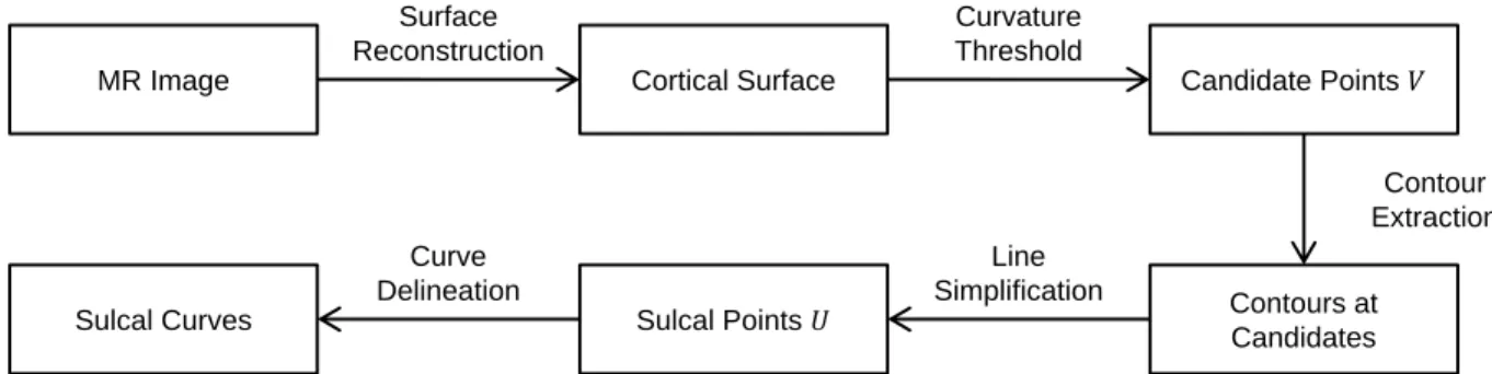
3.2
Objective
MR Image Cortical Surface Candidate Points ܸ
Contours at Candidates Sulcal Points ܷ
Sulcal Curves
Surface Reconstruction
Contour Extraction Curve
Delineation
Curvature Threshold
Line Simplification
Figure 3.1: A schematic overview of the sulcal curve extraction. For each candidate sulcal
point, a single contour is extracted. The line simplification is then employed to filter non-sulcal
candidates.
In the sulcal point extraction a set of candidate points is first selected via a relatively
generous thresholding of the maximum principal curvature at each location
∈
Ω. Then, a
cutting plane is computed such that it is orthogonal to the first principal direction at each
point
v
∈
V
, and the corresponding intersection is obtained between that plane and the
surface. A point is added to
U
if it is preserved after the line simplification process. In the
sulcal curve delineation, the selected points are connected using a geodesic kernel over Ω with
additional smoothing term. A schematic overview of the proposed method is illustrated in
Figure 3.1.
3.3
Slicing and Contour Extraction
given tangent direction
T
is obtained by
k(T) =
D
TN
·
T,
(3.1)
where
N
is the surface normal at
v. Since the objective is to check if
v
is potentially identified
as a sulcal point, a proper tangent direction
T
needs to be determined to find a maximum
curvature
k
in 2D space, in which the surface bends highly along its sulcal bank. The
maximum curvature is defined here along the direction associated with the second principal
curvature
k
2≥
k
1, where
k
1is the first principal curvature (see also Section 2.2 for details).
Thus, the first principal direction defines a plane for each vertex
v
∈
V
. Let
T
k1be the first
principal direction associated with
k
1at
v. Thus, the plane equation is given by
T
k1·
(x
−
v) = 0.
(3.2)
(a)
(b)
(c)
Figure 3.2: Contour extraction. (a) Schematic situation with dotted curves indicating several
cutting planes. (a) The second (maximum curvature) principal directions is colored by
red
,
respectively. (b) The cutting plane orthogonal to the second principal direction represents
a sulcal point with the maximum surface bend. (c) An example contour on actual cortical
surface (b) without the surface for better visualization.
synthetic and an actual cortical surface. The principal direction captures the maximum
curvature as an optimal representation of the sulcal fundus in terms of its surface bend.
3.4
Sulcal Point Detection
Once the proposed contour is obtained at
v
∈
Ω, my method applies the line simplification
approach to the contour to select the minimum sufficient number of extremal points that
represent the contour itself and to check if
v
is filtered out after the line simplification method,
as illustrated in Figure 3.3. Here is a brief summary of the line simplification method [103, 25].
For a given polyline, the two endpoints
p
0and
p
1are connected as a horizontal (base) line.
Then, the extremal point ˆ
p
along the polyline with the maximum distance from the line is
selected as follows:
ˆ
p
= argmax
p
k(p
1−
p
0)
×
pk · kp
1−
p
0k
−1
.
(3.3)
(a)
(b)
(c)
Figure 3.3: Sulcal point detection. (a) The contour that represents the maximum surface
bend at a query point is obtained with respect to the principal direction. (b) In order to
simplify the contour, the line simplification method selects a minimum sufficient number of
the convex (
red
) and concave (
blue
) points that are part of the original contour. (c) The
query point survives and is selected as a candidate point after the line simplification method.
(a)
(b)
(c)
(d)
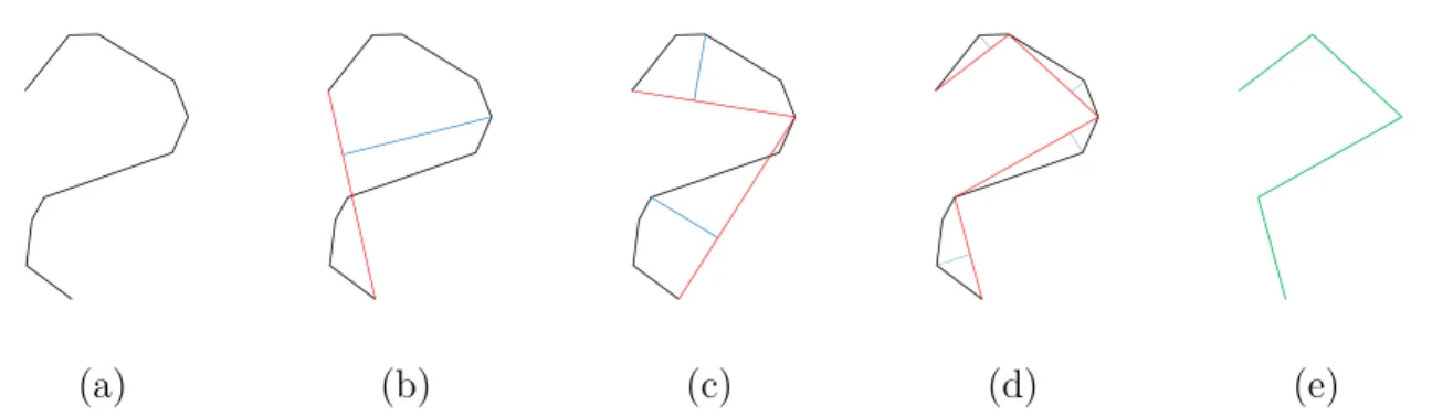
(e)
Figure 3.4: A schematic overview of the line simplification method. (a)-(b) Given a piece-wise
curve, a horizontal line (
red
) is obtained by finding the two farthest points, and the extremal
point is selected, having the farthest distance (
blue
) from the horizontal line. (c)-(d) The
selected extremal point is then employed to connect a new horizontal line and the procedure
is recursively applied until the distance from the horizontal line to a new extremal point is
below a threshold. (e) The final simplified line is obtained by connecting all the detected
extremal points.
than the maximum deviation [104], depending on the application. Figure 3.4 illustrates a
schematic overview of the line simplification method.
In this problem setting, two endpoints are determined by finding the largest distance on
the plane of
T
k2among all possible pairs of points on the contour to split it into two longest
method is then applied to one of the two curves that contains the testing point
v. If
v
is
reported as a local maximum by the line simplification method,
v
is collected into
U
as a
sulcal point. Overall, the proposed method collects a set of candidate points whose number
varies according to a user-defined threshold value. Figure 3.5 shows an example of candidate
points chosen by the line simplification method. Since potential sulcal points lie along valley
regions, they have a positive principal curvature. For expediting the process, the number of
tests is further reduced by choosing a generous thresholding of curvatures. In the experiment,
this threshold was empirically set to 0.01. Such thresholding is mainly for computational
time reduction.
3.5
Curve Delineation
In order to connect the candidate points into complete curves, potential endpoints of (yet
unknown) sulcal curves need to be estimated. For
∀u
∈
U
, thus, sulcal candidates points are
collected within a geodesic distance
r
defined by an indicator function:
R(u,
v) =
1
if
L
u(v)
≤
r ,
0
otherwise
,
(3.4)
where
L
uis a geodesic distance from
u
to
v
∈
Ω. The geodesic distance
L
ucan be computed
Figure 3.5: Maximum curvature points (
top
) and detected sulcal points (
bottom
, where sulcal
endpoints are colored in
green
and
blue
). The vertices with positive curvatures are selected
for candidate sulcal points. Since the candidate vertices are spread over a large portion of the
sulcal fundic regions, they are further filtered out by the proposed method that eventually
selects sulcal points (
blue
). The endpoints (
green
) are then selected from the selected sulcal
points.
Equation 2.15 becomes
F
x,
∇L
u(x)
k∇L
u(x)k
!
= 1.
(3.5)
For
M
=
I, this simplifies the H-J PDE to the Eikonal PDE:
The solution provides a geodesic distance
L
ufor all locations of Ω. The geodesic distance
r
in
Equation 3.4 is chosen under the assumption that the sulcal regions are separated from each
other by at least
r. In this chapter, this quantity was empirically set
r
= 4.0
mm
based on
the average width of the sulcal regions in the MNI-305 template [70]. This geodesic distance
can be adjusted depending on the target population.
The candidate points are determined as endpoints if every point holding
R(u,
·) = 1 is
located within an octant centered at
u
as shown in Figure 3.6. This is easily achieved by
testing the sign of the inner products of all neighboring points holding
R(u,
·) = 1, i.e., no
line between the neighboring points and the center point
u
has a separating angle above
90 degrees. Let
E
⊆
U
be the set of the endpoints determined by this way. To find the
neighboring sulcal point at
u
∈
E, the weighted shortest distance is employed from
u
to
s,
such that
s
holds
R(u,
s) = 1. The distance weighting is based on the assumption that the
tangent direction of the sulcal curve changes smoothly along the curve. Thus, the weighted
distance is given by the following form:
C(s,
u) =
k(s
−
u)
×
T(u)k
,
(3.7)
where
T(u) is the tangent vector at
u. Therefore, the neighboring sulcal point ˆ
s
at
u
is
obtained by
ˆ
s
= argmin
s
C(s,
u).
(3.8)
However,
T(u) is unknown due to no prior knowledge of the sulcal curve available. Instead
T(u) is estimated using the local principal direction,
T
k2(u). This is an incremental procedure;
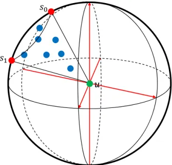
ݑݑ
ݏ
ݏ
ଵFigure 3.6: A schematic overview of the proposed endpoint detection. An example of the
octant of the sphere is determined by three orthogonal axes.
u
is determined as an endpoint
if its neighboring points in a geodesic kernel
S(u) belong to one of the octants.
us
0and
us
1form the maximum angle across every possible line starting from
u, such that
R(u,
s
0) = 1
and
R(u,
s
1) = 1.
R(ˆ
s,
·) = 1 and it stops if ˆ
s
∈
E
or ˆ
s
is a part of the other already delineated curve (junction
point). Starting at an arbitrary endpoint, the curve estimation is finished if every element in
E
has been connected. Figure 3.7 shows the estimated curves from sulcal points. The sulcal
endpoints are located in the end of each sulcal curve.
3.6
Materials
I chose the Kirby reproducibility dataset [53] to evaluate my sulcal extraction method
for reproducibility. Briefly, the Kirby reproducibility dataset was aquired on 21 healthy
volunteers with no history of neurological disease and is publicly available on NITRC
2.
Scan-2