EFFICIENT MOTION PLANNING FOR DEFORMABLE OBJECTS WITH HIGH DEGREES OF FREEDOM
Zherong Pan
A dissertation submitted to the faculty at the University of North Carolina at Chapel Hill in partial fulfillment of the requirements for the degree of Doctor of Philosophy in the Department of
Computer Science.
Chapel Hill 2019
c 2019 Zherong Pan
ABSTRACT
Zherong Pan: Efficient Motion Planning for Deformable Objects with High Degrees of Freedom
(Under the direction of Dinesh Manocha)
Many robotics and graphics applications need to be able to plan motions by interacting with complex environmental objects, including solids, sands, plants, and fluids. A key aspect of these deformable objects is that they have high Degrees of Freedom (DOF), which implies that they can move or change shapes in many independent ways subject to physics-based constraints. In these applications, users also impose high-level goals on the movements of high-DOF objects, and planning algorithms need to model their motions and determine the optimal control actions to satisfy the high-level goals.
ACKNOWLEDGEMENTS
I am grateful for the opportunity to work with Prof. Dinesh Manocha and Prof. Ming C. Lin. I joined UNC looking forward to a change in my career and their wise suggestions were invaluable while I shaped my research questions and dug up valuable problems to explore. Without their help, my accomplishments and this thesis would not have been possible. Prof. Manocha put a lot of effort into helping me, as an international student, build up my communication skills and conduct studies with collaborators both inside and outside UNC.
In addition to my advisors, I would like to thank my other committee members. Prof. Marc Niethammer taught me first course in image processing, through which I identified my first research project during my second year of Ph.D. study. I took two solid courses from Prof. Ron Alterovitz that laid the foundations for my robotic research. Prof. C. Karen Liu give me useful suggestions during my Ph.D. proposal and reading her insightful and inspiring research is always a delightful and helpful experience.
In addition, I received much help from my collaborators and friends in Chapel Hill. My friend, Tetsuya Takahashi, offered useful feedback and suggestions on a lot of my research. He also helped me proofread almost every one of my papers. We spent a lot of time together, talking about career, life, and everything else. My friend, Liang He, gave me useful life suggestions and I enjoyed travelling with him to explore different areas around Chapel Hill. Finally, all the other GAMMA members helped me in many ways, especially in improving my research work and broadening my horizons.
TABLE OF CONTENTS
LIST OF FIGURES . . . ix
LIST OF TABLES . . . xvi
LIST OF ABBREVIATIONS . . . xvii
CHAPTER 1: INTRODUCTION . . . 1
1.1 Components of Motion Planner for Deformable Objects . . . 3
1.1.1 Dynamic Models of Deformable Objects . . . 4
1.1.2 High-DOF Motion Planning Algorithms . . . 5
1.1.3 Acceleration Techniques for Dynamic Models . . . 6
1.1.4 Acceleration Techniques for Planning Algorithms . . . 7
1.2 Thesis Statement . . . 8
1.3 Main Results . . . 9
1.3.1 Planning Algorithms for Liquid Transfer . . . 9
1.3.2 Artist-Editable Fluid Animation . . . 10
1.3.3 Volumetric Elastically Deformable Character Locomotion . . . 11
1.3.4 Dynamic Models with Many Frictional Contacts . . . 13
CHAPTER 2: PLANNING ALGORITHMS FOR LIQUID TRANSFER . . . 15
2.1 Related Work . . . 16
2.2 Background: Liquid Dynamic Model . . . 16
2.3 Background: Optimization-Based Motion Planner . . . 20
2.4 Heuristic Planning Algorithm using Iterative Position Correction . . . 21
2.4.1 Results . . . 24
2.5 Convergent Planning Algorithm using Simplified Dynamic Model . . . 24
2.5.2 Results . . . 31
2.6 Feedback Motion Planning via Supervised Learning . . . 32
2.6.1 Training Data Generation . . . 35
2.6.2 Results . . . 36
2.7 Conclusion and Limitations . . . 39
CHAPTER 3: MOTION PLANNING FOR FLUID ANIMATIONS . . . 41
3.1 Related Work . . . 42
3.2 Background: Simplified Inviscid Fluid Model . . . 43
3.3 Background: Partial Differential Equation (PDE)-Constrained Trajectory Optimization 44 3.4 Overview of Our Approach . . . 45
3.5 Solving the Advection Optimization (AO) Subproblem . . . 46
3.6 Solving Navier-Stokes Optimization (NSO) Subproblem . . . 49
3.6.1 Full Approximation Scheme . . . 50
3.7 ADMM Outer Loop . . . 53
3.8 Results and Analysis . . . 53
3.9 Conclusion and Limitations . . . 60
CHAPTER 4: MOTION PLANNING FOR VOLUMETRIC ELASTICALLY DE-FORMABLE OBJECTS . . . 65
4.1 Related Work . . . 66
4.1.1 Background: Optimization-Based Motion Planner Using Soft Constrained . . 67
4.1.2 Background: Parameterization of Configuration Spaces . . . 67
4.2 Objective Function Terms . . . 69
4.2.1 Physics-Based Constraints . . . 69
4.2.2 Environmental Force Model . . . 71
4.2.3 Controller Parametrization and Shuffle Avoidance . . . 73
4.3 SpaceTime Optimization . . . 76
4.3.1 Hybrid Optimizer . . . 76
4.3.2 Efficient Function Evaluation . . . 77
4.4 Results and Evaluations . . . 81
4.4.1 Combining our Algorithm with Partial Keyframe Data . . . 85
4.5 Conclusion and Limitations . . . 87
CHAPTER 5: DYNAMIC MODELS WITH MANY FRICTIONAL CONTACTS 90 5.1 Background: Newton-Euler’s Equation . . . 91
5.2 Background: Time-Integrating Frictional Contact Forces . . . 92
5.3 Position-based Articulated Object Dynamic Model . . . 93
5.3.1 High-Order Position-Based Collocation Method . . . 94
5.3.2 Optimization Algorithm . . . 95
5.3.3 Algorithm Complexity of High-Order Collocation Methods . . . 98
5.3.4 Graphics Processing Unit (GPU) Parallelization . . . 98
5.4 Frictional Contact Model for Position-Based Articulated Object Dynamic Model (PBAD) . . . 100
5.4.1 Normal Force Model for PBAD . . . 101
5.4.2 Tangential Force Model for PBAD . . . 102
5.4.3 Comparison with Dry Frictional Model . . . 103
5.5 Evaluations Without Frictional Contact Forces . . . 104
5.6 Evaluations With Frictional Contact Forces . . . 107
5.7 Conclusion and Limitations . . . 109
CHAPTER 6: CONCLUSION AND FUTURE WORK . . . 110
6.1 Limitations . . . 111
6.2 Future Work . . . 111
LIST OF FIGURES
1.1 We illustrate applications of motion planning for high-DOF robots or with high-DOF passive environmental objects. (a): Planning the motion of a spoon of liquid to avoid spillage, where the liquid is the passive environmental object and is modeled with 100 thousand DOFs (Kuriyama, Yano, and Hamaguchi2008). (b): A robot manipulating a piece of cloth, where the cloth is the passive environmental object and is modeled with 1 thousand DOFs (A. X. Lee, Lu, et al. 2015). (c): A physical soft crawling high-DOF robot whose motions are manually designed (Shepherd et al. 2011). (d): Computer generated fluid animations that are editable by artists, where the fluid is the high-DOF robot and is modeled with 5 million DOFs (Shi and Yu2005). . . 2 1.2 In our first problem, we has a robot arm hold a source container in which there is a
body of liquid. The goal is to compute a motion planner for the source container so that the body of liquid is transferred into the target container. . . 9 1.3 Our second problem is to plan motions for fluid animations such that the fluid takes
a particular shape (letter A, B, and C) while preserving the fine details (while circles). 10 1.4 Our third problem is to plan locomotion trajectories for boneless deformable characters
such as a single-legged T-shape jumping (a), a four-legged spider walking (b), and a fish swimming (c). These characters have a number of DOFs, N >1000. . . 12 1.5 All the characters in this figure have low-DOF by themselves, i.e. N ≤20, but they
have many points of contact with the environment. Handling these contacts can become a computational bottleneck. . . 13
2.1 We ran5 passes of 2D liquid simulations with same initial setting: pouring a cup of water. For each larger i, we double the resolution and halve the particle radius. A mesh is reconstructed for each timestep in each simulation (purple). . . 18 2.2 (a): Error plot formesh(i, t), i= 1,· · ·,4with respect to timestept. As iincreases,
the error is approximately halved. (b): Number of particles whose streamline can be approximated by a quadratic curve with error less than , plotted against the total number of particles used in simulation. We chooseequals to particle radius in all the experiments. . . 19 2.3 Each particlepj is associated with a streamlinePj, which is comprised of three stages.
The particle is within the source container during the first stage (red), free-flying in air during the second stage (green), and inside the target container during the third stage (blue). We requirePj to pass through the center of the rectangular target container openingc. . . 21 2.4 Different timesteps i of the optimized liquid trajectory Pk after k iterations of
Algorithm 2, where we use a small dynamic viscosity coefficientµ= 0.01. The error reduces significantly after 1 iteration from Q2 to Q3. . . 24
2.5 Different timesteps i of the optimized liquid trajectory Pk after k iterations of Algorithm 2, where we use a large dynamic viscosity coefficient µ= 0.5 for the liquid. The error reduces significantly after 5 iterations. . . 25 2.6 Different timesteps i of the optimized liquid trajectory Pk after k iterations of
2.7 Different timesteps i of the optimized liquid trajectory Pk after k iterations of Algorithm 2, where we use a large dynamic viscosity coefficient µ= 0.5 for the liquid. Same as the case with Figure 2.5, error reduction is slower, taking 4 iterations. . . . 27 2.8 (a): An illustration of the parameters related to the source container. The cross
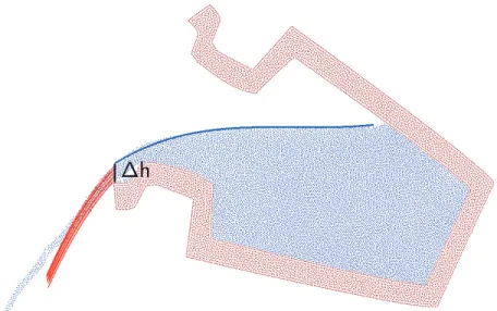
section area A is the shaded region with centroid e. The outflowing velocity has magnitudevout. (b): The outflow direction is horizontal when θ <90◦. Otherwise, it is along the tangent direction. . . 28 2.9 (a): Illustration of functionA(θ,vol). (b): Illustration of function ∆h(θ,vol). (c,d):
More examples for containers of different shapes. A watershed algorithm is used to extract the interior of the source container (blue) and to populate the lookup table of A(θ,vol) (colormap). The same procedure is used to precompute∆h(θ,vol) on the axial symmetric cross section. . . 29 2.10 The two physically inspired approximations. (a): The Bernoulli equation is used
between two end points of the dashed streamline. (b): A single liquid particle sliding down the wall of the container. . . 29 2.11 A snapshot of the cross section of liquid simulation, the extracted quadratic curves
(red) for particles leaving the source container at the current timestep. Their tangents are averaged to compute vout, and the cubic curve fitted to the free surface (blue). This is used to compute∆h by evaluating the free surface position at the boundary of the source container. . . 30 2.12 For two simulated testing trajectories and two container shapes, we plot changes
of the five variables vout,p
2kgkh, θ,∆h and g(θ,vol) over time. Both testing and training trajectories are generated by simulating the liquid while tilting the container according to a random, monotonically increasing θcurve shown in orange. The green curve is the groundtruthvout, the outflowing velocity magnitude; the gray curve is the groundtruth∆h, and the yellow curve is the prediction of vout made by the Bernoulli equationp2kgk∆h. Finally, the blue curve is the predicted vout generated using our simplified dynamic modelg(θ,vol). The error betweenvout andg(θ,vol)is small over the effective range wherevout>0. . . 31 2.13 We use our simplified dynamic model Equation 2.11 to simulated a simplified
tra-jectory and plot the syntheticvout as (green). Over time, the tilt angle θ increases monotonically (orange) while the total volume decreases accordingly (yellow). Note that the change of vout (green) closely resembles the groundtruth data (Figure 2.12 green): for the cylindrical container,vout is always increasing while for the oval-shaped container,vout first increases and then decreases. . . 32 2.14 An illustration of our feedback motion planning framework. From the training dataset
found by stochastic optimization (a), we train a neural network that predicts key parameters in the formulation ofCOBJ and CPDE (b). Our online planner then uses COBJ and CPDE and solves Equation 2.4 in a receding-horizon manner (c). . . 33 2.15 (a): Our 4-layer neural network structure for parameter estimation. The input is an
2.16 We illustrate an exemplary trajectory of TRANSFER+FOLLOW (a) and TRANS-FER+ZERO (b). On convergence of CMA-ES optimization, the liquid flow is well centered around the opening ofc (c). Problems in TRANSFER+ZERO are more challenging because liquids are more likely to spill at an early stage of transfer (d), so that the source container must be moved and tilted slowly (e). For each timestep in each trajectory, we extract the ground truth water heightfield and the outflow quadratic curve as training dataset (f). . . 37 2.17 (a): The scaled reward function R/#P article for a set of transfer problems in
TRANSFER+FOLLOW (blue) and TRANSFER+ZERO (red). These values are all positive, meaning that very little spillage happens and particles are well centered aroundc. (b,c): The average convergence history of CMA-ES algorithm over 1000 problems. This algorithm converges equally well for TRANSFER+FOLLOW (b) and TRANSFER+ZERO (c). . . 38 2.18 Performance of feedback planner. (a): The fraction of spilled particle using rectangular
containerS, two kinds of datasets and features. (b): The fraction of spilled particle using height at lip feature and three different container shapes. (c): Average reward of particles that fall into the target container in experiment (a). (d): Average reward of particles that fall into the target container in experiment (b). . . 38
3.1 Given a set of keyframes, we use an optimization-based motion planner to compute a dense sequence of control force fields, matching a smoke ball to the word “FLUID.” We highlight the control force fields. Five such animations are generated at resolution1282 with 40timesteps. Each of these optimization computations takes about 0.5(hr) on a desktop PC and is about17×faster than a conventional gradient-based, optimization-based motion planner. . . 41 3.2 We tested the fixed point iteration Equation 3.6 using different advection operator
A[•,•] to deform an initially circle-shaped smoke (top left) into the bird icon (bottom left). The AO subproblem solved using the semi-Lagrangian operator involves lots of popping artifacts (top row). The upwinding operator in Equation 3.2 does not suffer from such problems (bottom row). . . 48 3.3 A 2D illustration of Full Approximation Scheme (FAS). We use semi-coarsening only
in the spatial direction (horizontal), with each finer level doubling the grid resolution. We use trilinear interpolation operators forP,R and tridiagonal SCGS smoothing for S, which solves the primal variables qi,ui (defined on faces as short white lines) and dual variables ψi,ψ¯i (defined in cell centers as black dots) associated with one cell across all the timesteps (vertical) by solving a block tridiagonal system. The solve can be made parallel by the 8-color tagging in 3D or4-color tagging in 2D. . . 50 3.4 Convergence history of FAS compared with that of the Limited-Memory
Broyden-Fletcher-Goldfarb-Shanno (LBFGS) optimizer, running on two grid resolutions and with a different number of timesteps (denoted as nd/N). FAS achieves a linear rate of error reduction independent of grid resolution and number of timesteps, as the two curves overlap. . . 51 3.5 We profile the convergence history of the example Figure 3.1. We plot the logarithm of
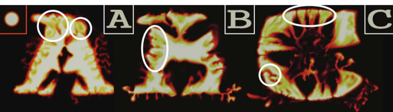
3.6 For this animation, we match the circle (red) first to two smaller circles and then to a bunny (we show frames20,40,60,80 from top to bottom). The resolution is 1282/80, and we test three different values of ghost force regularizationr = 102,3,4 (from left to right). More smoke-like behaviors are generated as we increaser. . . 56 3.7 In this example, we deform a sphere into letter “A”, then letter “B” and finally letter “C”.
For such a complex deformation, it is advantageous to allow every velocity component to be optimized. So that a lot of fine-scale details can be generated as illustrated in the white circles. . . 57 3.8 3D smoke control example of deforming a sphere first to an armadillo and then to a
bunny. This example runs at the resolution of643with40timesteps. The optimization
can be accomplished in7(hr). . . 57 3.9 We generate the famous example of tracking smoke with a dense sequence of keyframes,
which comes from human motion capture data. Our algorithm converges and generates rich smoke drags within 5 ADMM iterations. . . 58 3.10 Example of smoke control where the keyframes have varying genera. The initial frame
is a sphere (genus 0). The first keyframe located at frame 20 is a torus (genus 1) and the second keyframe located at frame 40 is the shape eight (genus 2). The resolution is642×32/40 and the overall optimization takes5(hr) with r= 103. . . 58 3.11 A moving smoke sphere guided by the 3 keyframes (left). We experimented with
r= 103 (top) and r = 104 (bottom). Larger regularization results in more wake flow behind moving smoke objects. The same effect can be observed in Figure 3.6. . . 59 3.12 Convergence history of the NSO solver in the Circle Bunny example. When the
regularization coefficientr is extremely large, we have to treat the FAS-VCycle as a subproblem solver of the Levenberg-Marquardt (LM) algorithm and the entire NSO solve requires many more FAS-VCycles. . . 60
4.1 The deformable object is represented as a triangle mesh (a). With a deformation bases set (b), its position is parameterized by local deformation u, a global rigid translation c (c), and rotationw (d). The Euclidean coordinates of jth vertex vj (blue dot) can be recovered by transformation function vj(p). . . . 68 4.2 To resolve collisions between thin components (a), we use approximate continuous
collision handling (b). . . 70 4.3 Fluid drag force is applied on each surface patch (va,vb,vc). The force strength
depends on the surface normaln and relative velocityU (a). We also plot the force strength with respect to tangential relative velocityUk and normal relative velocity U⊥. Our new formulation isC1-continuous (b), while the original formulation has a
discontinuous gradient (c), especially when the relative velocity is almost tangential (shown with a red box). . . 73 4.4 A letter T jumping forward. With Dynamic Movement Primitives (DMP)
regulariza-tion termCDMP, its center of mass (blue) traces out a periodic trajectory. . . 74 4.5 Frames highlighting the dragon walking trajectory using our approach. In the result
4.6 For the spider (top) and fish (bottom) models (a), we visualize the kinetic cubatures (b) and surface patch cubatures (c). In both cases, only a small fraction of elements need to be considered for the summation. This fraction is 12%for the spider and 0.7%for the fish model. . . 78 4.7 When user sets a target point (green) too far away (5meters to the right) and uses
very few timesteps (20in this case), the Letter T chooses to lean itself too much to recover from falling down. . . 80 4.8 We show two swimming trajectories optimized using static initialization (a) and
random initialization (b). For both trajectories, we plot the locus of the deformable object’s center of mass (white curve) and the magnitude of control forces in (c,d). The goal is to move 5 meters to the left after 10 seconds. Our optimizer finds two different but almost equally effective gaits. . . 81 4.9 We plot the convergence history using static initialization (a) and random initialization
(b). Both optimizations reduce the objective function to less than 1%of the original value. This plot shows that many local minima of our objective function leads to plausible animations. There are some jittering during the optimization. This is because the adaptive penalty method (Algorithm 6) is adjustingWDMP. . . 82 4.10 We use Rapidly-Exploring Random Tree (RRT)* to navigate physical swimming
characters, the fish (a) and the spider (b), to look for food plants (green). The white line is the locus of the deformable object’s center of mass computed using RRT*. . . 84 4.11 The spider walking on planar ground (a) and V-shaped ground (b). . . 85 4.12 Different frames during a beam jumping with different target altitudes (yellow arrow);
(a): h= 2, (b): h= 3, and (c): h= 4. . . 86 4.13 Different frames during a beam jumping forward with different target distance (yellow
arrow); (a): kvck= 2, (b): kvck= 2.5, and (c): kvck= 3 (the target altitude h= 3). 86
4.14 (a): An X-shaped deformable body walking by rolling. (b): The rest shape. . . 87 4.15 To compute the navigation path for the spider, we optimize 3 trajectories: swimming
forward (a), turning left (b), and turning right (c) (the timestep index increases along the arrow, and the white bodies mark the most deformed configurations). These differences in the gaits can be represented by different DMP parametersαnandβn only. 87 4.16 We show a walking dinosaur guided by both our high-level objectives and
user-specified keyframes in (a) so that its head is looking around, and the upper-body partial keyframes are illustrated in (b,c). Each of these keyframes contains 788of the 1493vertices. . . 88
5.1 An illustration of our GPU implementation. The GPU hasM cores, each illustrated as a gray box on the left. We use a workgroup ofN cores (black arrow) to simulate one trajectory. In this illustration, we compute 3 trajectories that each have 4 timesteps (p2,· · · ,p5). During each call to the GPU, instead of finishing the entire
LM optimization, we compute just one iteration of the LM optimization (colored block on the right) so that all the workgroups are running the same computation and no starvation will happen. Different timesteps are illustrated using blocks of different colors. For example, it takes2iterations to compute p2 in the first trajectory and7
5.2 The penetration depth,dist(X(p)), at point Xis the magnitude of the blue vector. We plot the change of dist(X(p)) as the red curve, which is a piecewise smooth function. Here the obstacle is the hatched area and n is the unit outward contact normal. . . 100 5.3 (a): We plot the total kinetic+potential energy over time during a standard simulation
of a 10-link chain that swings downward. Each joint of this chain is a 2-DOF ball joint so that this chain has 20-DOF. Forward Euler integrator for the Newton-Euler equation and semi-implicit Euler integrator are not stable. Being fully implicit, our second-order PBAD solver is stable but quickly loses energy. By increasing the order by one, both the second-order Runge-Kutta and our third-order PBAD solver preserve energy very well. (b): For the more challenging problem of a 100-link chain (200-DOF) that swings downward, even the second-order Runge-Kutta method is not stable and we have to use the third-order Runge-Kutta method for better energy preservation. Our second-order PBAD solver is stable but quickly loses energy. Our third-order PBAD solver preserves energy very well. (c): We compare the total computational time for generating a10s trajectory of a 10-link chain swinging down using a second-order collocation method for PBAD and a semi-implicit Euler integrator for a conventional formulation. PBAD is 1.5−2.1 times slower at a small timestep size and up to 4 times faster at a large timestep size, such as 0.05s. . . 104 5.4 We compare the performance of the two optimization algorithms (LM and LBFGS)
during the simulation of a 10-link (20-DOF) (a) and a 40-link (80-DOF) chain (b) with a large timestep size of 0.05s. The number of iterations used by LBFGS is much larger than that used by LM, although each iteration of LBFGS is cheaper. In addition, the number of iterations is almost independent of the number of links, N. (c): We plot the average time to finish one step of the simulation against the number of links, N. LBFGS is comparable to LM in terms of computational time and the computational time grows almost linearly with N in the range of N = 10−40. (d): We plot the average time to finish one step of the simulation against the timestep size,∆t. PBAD can be used with very large timestep sizes and we tested ∆t= 0.001,0.002,0.004,0.008,0.016,0.032,0.064,0.128s. The computation time for each timestep is almost invariant to∆t. . . 105 5.5 We compare the performance of CPU and GPU in simulating a chain swinging
benchmark. (a): We plot the speedup against the number of links, N. The speedup increases withN and the maximal speedup over a 4-core CPU is6 times. (b): When N = 10, we plot the speedup against the number of trajectories. The speedup also increases with the number of trajectories and the maximal speedup is4 times. (c): We plot the total computational time against the number of links,N, for generating 100 trajectories of 10 timesteps each. When N = 40, the 100 trajectories can be generated in less than1s on GPU. (d): We plot the total computational time against the number of trajectories. . . 106 5.6 (a): We simulate a box sliding on the ground with an initial velocity of 1m/s, using
5.7 (a): A 10-link chain sliding off a slope. (b): Time cost to compute a 10s trajectory plotted against timestep size. Conventional formulation is stable only when ∆t < 0.0025s. (c): Time cost plotted against the average number of contact points (more contact points derived by refining the mesh). (d): Time cost plotted again the frictional coefficient (µ for the dry frictional model,Ck for our formulation). . . 108 5.8 We run two Reinforcement Learning (RL) benchmarks, 2D-hopper (a) and 3D-walker
LIST OF TABLES
1.1 The number of DOFs, N, and the material types of dynamic models proposed by representative previous methods. . . 5
2.1 Parameters used in our liquid simulator: Average particle radius, gravity, time step size, number of particles needed to fill the long bottle, number of particles needed to fill the cup with handle, total number of timesteps, and maximal iterations count. . . 23 2.2 From left to right: benchmark environment, viscosity of liquid, time spent solving
Equation 2.4, time spent running forward liquid simulation for validation and quality of planned trajectory. The quality is measured by the fraction of particles that fall inside target container. . . 32
3.1 Parameters. . . 53 3.2 Memory and computational overhead for all the benchmarks. From left to right: name
of example (resolution parameters); the spatial boundary condition; number of outer ADMM iterations; average time spent on each AO subproblem; average time spent on each NSO subproblem; total time until convergence using our algorithm; memory overhead; total time until convergence using LBFGS. By comparing the three “Circle Bunny” examples, we can observe that the number of ADMM outer loops is roughly linear tolog10(r). More ADMM outer loops are needed, if more fluid-like behaviors are desired. From the two examples of the Letters “FLUID” (Line 1 and Line 2), we can observe that the computational cost of each ADMM outer loop (Avg. AO + Avg. NSO) is roughly linear in the number of timesteps. This cost is also closely related to the number of keyframes. By comparing Line 2 and Line 4, we can observe that the Circle Bunny example which involves two keyframes requires more computation to solve the NSO subproblem. . . 55
4.1 Performance of LBFGS and our hybrid solver on two examples: 2D worm crawling and 2D ball rolling. Our approach is significantly faster. . . 76 4.2 Parameters. . . 82 4.3 Benchmark setup and computational overhead. From left to right, number of vertices
V/number of Finite Element Method (FEM) elementsP, DOFs of local deformation |u|, precomputation time for building reduced dynamic model/computing surface patch cubatures, number of frames/number of trajectories, time spent on optimization, and the supported application: DMP means we use DMP as open-loop controller to control realtime forward simulation, FB means that we use feedback controller to track the animation (both of these are realtime). . . 83
LIST OF ABBREVIATIONS
ADMM Alternating Direction Method of Multipliers.
AO Advection Optimization.
BEM Boundary Element Method.
CCD Continuous Collision Detection.
CIO Contact Invariant Optimization.
DI Differential Inclusion.
DMP Dynamic Movement Primitives.
DOF Degrees of Freedom.
FAS Full Approximation Scheme.
FEM Finite Element Method.
FST Fast Sandwich Transform.
GPU Graphics Processing Unit.
GS Gauss-Seidel.
KKT Karush-Kuhn-Tucker.
LBFGS Limited-Memory Broyden-Fletcher-Goldfarb-Shanno.
LCP Linear Complementary Problem.
LICQ Linear Independence Constraint Qualification.
LM Levenberg-Marquardt.
LQR Linear Quadratic Regulator.
MPC Model Predictive Control.
NS Navier-Stokes.
NSO Navier-Stokes Optimization.
PBAD Position-Based Articulated Object Dynamic Model.
PD Proportional-Derivative.
PDE Partial Differential Equation.
POD Proper Orthogonal Decomposition.
QCQP Quadratically Constrained Quadratic Programming.
QP Quadratic Programming.
RL Reinforcement Learning.
RRT Rapidly-Exploring Random Tree.
RS Rotation-Strain.
SCGS Symmetric Coupled Gauss-Seidel.
STFAS Spacetime Full Approximation Scheme.
CHAPTER 1
Introduction
(a) (b) (c) (d)
Figure 1.1: We illustrate applications of motion planning for high-DOF robots or with high-DOF passive environmental objects. (a): Planning the motion of a spoon of liquid to avoid spillage, where the liquid is the passive environmental object and is modeled with 100 thousand DOFs (Kuriyama, Yano, and Hamaguchi 2008). (b): A robot manipulating a piece of cloth, where the cloth is the passive environmental object and is modeled with 1 thousand DOFs (A. X. Lee, Lu, et al. 2015). (c): A physical soft crawling high-DOF robot whose motions are manually designed (Shepherd et al. 2011). (d): Computer generated fluid animations that are editable by artists, where the fluid is the high-DOF robot and is modeled with 5 million DOFs (Shi and Yu2005).
Aribowo, Yamashita, and Terashima 2015), deformable objects are modeled as passive objects that can be manipulated. High-DOF robots or passive objects in these applications pose new challenges for motion planning algorithms as highlighted below.
• Dynamic Modeling: Many planning algorithms, e.g. Model Predictive Control (MPC) (Mayne 2014), rely on the predictions of robot or passive object motions given the control inputs. Such predictions are accomplished using a dynamic model. Unlike point-shaped, disk-shaped, or articulated robots, the dynamic behaviors of high-DOF deformable objects are more difficult to model because they are infinite-dimensional (J. Huang et al.2019), so that discretizations are needed to derive a finite-dimensional model, which in turn introduces discretization errors. On the other hand, when the deformable objects can be controlled, additional actuation structures, such as muscles, rigid bones, and cables, are used. These actuation structures make motion planning easier but their dynamic behaviors are hard to model, as multi-physics dynamic models are required (Michopoulos, Farhat, and Fish2005). • high-DOF Planning Algorithms: Almost all planning algorithms have complexities that
are superlinear inN. For example, solving the optimal control problem using Linear Quadratic Regulator (LQR), which assumes a linearized dynamic model and a quadratic cost model, incurs a complexity of O(N3)(Benner, Görner, and Saak 2006). Algebraic methods have an
and Amato2006; Moll and Kavraki2006) can be used for any robot or passive object, but they also have a superlinear complexity in N (Hopcroft, Schwartz, and Sharir1984), so they are only useful in low-DOF cases. Therefore, a major challenge in planning algorithms lies in the handling of high-DOF configuration spaces.
• Planning for Non-smooth Dynamic Models: Planning problems become more challenging when non-smooth changes in the deformable objects are considered. Examples of non-smooth changes include changes in the boundary condition such as contact with obstacles (Posa, Cantu, and Tedrake 2014) and fluid-solid-air interface changes (Rasmussen et al. 2004). To model non-smooth changes, e.g. for walking and climbing robots, direct methods (Posa, Cantu, and Tedrake 2014) introduce hard constraints into trajectory optimization for each possible case where a non-smooth change can happen. For high-DOF deformable objects, the number of hard constraints can increase considerably. Stochastic methods such as (Kalakrishnan et al. 2011) treat the non-smooth dynamic model as a black-box and probe the performance of a
motion plan by sampling, but little analysis has been performed on the algorithmic complexity in terms of N.
• Realtime Performance: In a virtual environment, users can interact with deformable characters using various input devices. These deformable characters should respond in a controlled manner at realtime framerates. When a physical robot collaborates with humans to manipulate a piece of cloth (Jia, Hu, et al. 2018), the robot should react to the human’s hand movements interactively. Offline open-loop motion planning algorithms (LaValle 2006) do not meet these performance requirements, and we therefore need online closed-loop motion planning algorithms (Mayne 2014). However, numerical simulations of deformable objects are computationally demanding (J. Huang et al. 2019). Online MPC algorithms (Mayne2014) are based on these simulation results and they also fail to meet realtime performances.
1.1 Components of Motion Planner for Deformable Objects
we formally define these components and discuss prior methods. 1.1.1 Dynamic Models of Deformable Objects
In the continuous setting, a deformable model takes up a bounded subset of the Euclidean workspace. Under a deformation, each point in this subset will translate to a different location. Therefore, the configuration of a deformable model is infinite-dimensional (Logg, Mardal, and Wells 2012). The foremost step in deriving a dynamic model is to propose a finite-dimensional approximation of the configuration space. This can be achieved using two methods. The FEM (Logg, Mardal, and Wells 2012) embeds the configuration space into a finite-dimensional function space. This method is general enough to model deformable objects with inhomogeneous materials. Under special assumptions, e.g., the material of deformable objects is homogeneous, the Boundary Element Method (BEM) (Bonnet, Maier, and Polizzotto1998; James and Pai1999) can be used to embed the configuration space into a finite-dimensional space of fundamental solutions. The finite-dimensional representation of FEM and BEM can be constructed for different geometric representations of deformable objects, including mesh-based (Ho-Le1988), meshless (Gu 2005), and spectral (Patera 1984) representations. Equipped with a finite-dimensional space, FEM and BEM then model the
materials of a deformable model by deriving the strain-stress relationship, i.e. the constitutive laws. The constitutive laws for common deformable objects such as Eulerian fluids (Harlow and Welch 1965), viscoelastic materials (Reese and Govindjee 1998; Bonito, Picasso, and Laso2006), elastically
deformable materials (Logg, Mardal, and Wells2012; Fung, Tong, and Chen 2017), and fracturing materials (Francfort and Marigo1998; Schlangen and Garboczi1997), have been well-studied and numerical schemes have also been developed for computational simulations.
Previous Method Deformable Object Material N (Gayle, Segars, et al. 2005) Elastically Deformable Objects 1280-10080
(Pauly et al.2005) Fracturing objects 4300-6500 (Foster and Fedkiw 2001) Eulerian Fluids 1687500
Table 1.1: The number of DOFs, N, and the material types of dynamic models proposed by representative previous methods.
1.1.2 High-DOF Motion Planning Algorithms
We assume that deformable objects can be modified by applying control signals. These control signal can take various forms, such as applying external wind forces to a volume of Eulerian fluids (Treuille et al.2003), applying actuating muscle forces (Tan, Turk, and C. K. Liu2012b) or cable pulling forces (Skouras et al.2013) to an elastically deformable object, and applying pressure forces to pneumatic robots (L.-K. Ma et al. 2017). In any case, motion planning algorithms are needed to compute the control signals that accomplish a high-level objective specified by users. This objective can be a goal position of locomotions (Tan, Turk, and C. K. Liu2012b), a quasistatic pose to be taken (Skouras et al. 2013), or a transient shape to be taken at a certain time instance (Treuille et al. 2003). To compute motion plans for these deformable objects, a practical algorithm must be able to handle the high-DOF of the configuration spaces as well as the dynamic constraints of the underlying physically-based models.
Many motion planning algorithms (LaValle 2006; Mayne 2014) are designed for handling general nonlinear dynamic models in configuration spaces of arbitrary dimensions. However, according to the classical analysis, their complexity with respect to N is superlinear (Benner, Görner, and Saak2006; Canny 1988; Hopcroft, Schwartz, and Sharir1984). As a result, these motion planning algorithms are only practical whenN <100, which has a big gap from the range ofN considered in our problems. Previous methods (Rodriguez, Jyh-Ming Lien, and Amato 2006; Moll and Kavraki 2006; Coros et al.2012; Patil et al. 2011) that apply these algorithms directly to deformable objects
can only handle robots represented using coarse meshes. Many works on deformable robot design rely heavily on human experiences (L.-K. Ma et al. 2017) and bio-inspired heuristics (Fras et al. 2018; Shepherd et al.2011) to specify the movement patterns of the robot. Other methods (Gayle,
An important type of motion planning algorithms that can potentially scale to high-DOF configuration spaces are the optimization-based local planning algorithms (Kalakrishnan et al. 2011; Schulman, Duan, et al. 2014; Treuille et al. 2003) and controller optimization techniques (Peters and Schaal 2006; Levine and Koltun2013; Schulman, Levine, et al.2015). Unlike global planning algorithms (LaValle 2006; Canny 1988), local algorithms sacrifice the completeness guarantee. However, backed by recent advances in large-scale numerical optimization (Gill, W. Murray, and Saunders 2005; Bottou, Curtis, and Nocedal 2018), these algorithms can search in the space of millions of variables with practical performance. In addition, they can take possible non-linear, non-smooth constraints, making these methods well-suited for large-scale motion planning under dynamic constraints. The benefits of local and global methods have recently been combined in (Kuntz, Chris Bowen, and Ron Alterovitz2017) where the local planner refines a sampled solution
from the global motion planner.
1.1.3 Acceleration Techniques for Dynamic Models
Acceleration techniques are needed to meet additional requirements on the efficiency of motion planning algorithms. For example, control signals must be computed within less than a second in closed-loop motion planning. Even in offline open-loop motion planning, the time to compute a motion plan must be less than the cost of manual design to make the algorithm practically useful. Acceleration techniques can be divided into two categories: accelerations for dynamic models and accelerations for planning algorithms.
For planning algorithms such as MPC (Mayne 2014; Tassa, Erez, and Emanuel Todorov2012; Hämäläinen, Rajamäki, and C. K. Liu2015), the cost to simulate the dynamic models dominates the computation. Therefore, we can achieve higher efficiency by accelerating the computational procedure of numerical simulations. For deformable objects, many previous works have contributed to this end. The large-scale linear system solvers required by FEM can be accelerated by iterative methods (Elman, Silvester, and Wathen2014), multigrids (Ruge and Stüben1987) and domain decompositions (Toselli and Widlund2006). The linear system solve required by BEM can be accelerated by fast multipole expansions (Darve 2000) and hierarchical matrices (Börm, Grasedyck, and Hackbusch 2003). For special dynamic models, we can develop customized acceleration techniques to obtain
and does not require re-factorization. For scenarios that do not require high accuracy in terms of numerical simulations, a large-scale linear system solve can be avoided by only applying local corrections, leading to position-based dynamic models (Bender, Müller, and Macklin2017).
On the other hand, due to the superlinear dependency of planning algorithms on N, acceleration can be achieved by reducing N of the dynamic models. This can usually be achieved by embedding the configuration space of a dynamic model into a low-dimensional feature space, which captures the salient characteristics of the original high-dimensional data that are important to planning algorithms. There are several methods to achieve this goal for general dynamic models of any kind. One example is the Koopman operator (Korda and Mezić 2018), which captures the linear observations from nonlinear dynamic models. Although the finite-dimensional Koopman operator is only available for certain dynamic models (Brunton et al.2016), machine learning can be used to approximately compute this operator (Lusch, Kutz, and Brunton 2018). Another example is Proper Orthogonal Decomposition (POD) (Chatterjee2000), which embeds the configuration space into linear subspaces spanned by orthogonal bases. This technique has been applied to elastically deformable objects (K. K. Hauser and Shen 2003) and Eulerian fluids (De Witt, Lessig, and Fiume2012), which can
then bring significant accelerations to planning algorithms (Barbič, Silva, and J. Popović 2009). 1.1.4 Acceleration Techniques for Planning Algorithms
In the previous section, we discussed acceleration techniques that work by approximating physics-based or dynamic models that can be used for faster computations. Better efficiency can also be achieved by accelerating the planning algorithms. Most previous works in this direction focus on sampling-based motion planners. Acceleration can be achieved by reducing the number of samples by inferring the effectiveness of new samples (Ichter, Harrison, and Pavone 2018; Jia Pan and Manocha 2016), learning a prior sampling distribution (C. Bowen, Ye, and R. Alterovitz 2015), relaxing the
optimality criterion (Salzman and Halperin2016), reducing the number of collision checks (K. Hauser 2015), or removing unnecessary samples (Gammell, Srinivasa, and Barfoot 2014; Karaman, Walter,
et al. 2011). However, all these methods have superlinear complexity in N so that they quickly become impractical for high-DOF deformable objects.
Kuindersma 2018; Park, Jia Pan, and Manocha 2013) or by using parallel scheduling of motion planning and execution (Park, Jia Pan, and Manocha2014). However, there is a recent resurgence in this direction with advances in deep learning, especially reinforcement learning. Reinforcement learning performs offline controller optimizations (Peters and Schaal2006; Levine and Koltun2013) and these controllers can be used online to achieve realtime performance. Alternatively, robots can learn from demonstrations (Schaal 1997; Ijspeert et al. 2013; Ho and Ermon2016) using offline planning results as experts. Deep system identification (Lenz, Knepper, and Saxena 2015) learns a surrogate dynamic model that provides efficient predictions to MPC. Most learning-based techniques have been adapted to planning motions in high-DOF configuration spaces. End-to-end neural networks can represent controllers from image-based observations (Levine, Finn, et al.2016). System identification has been used to learn the dynamic behaviors of 3D Eulerian fluids (Wiewel, Becher, and Thuerey 2019).
1.2 Thesis Statement
Our thesis statement is as follows:
Planning for high-DOF deformable objects such as fluids and elastically deformable objects can
be accelerated by exploiting dimension reduction, machine learning, and hierarchical representation,
and can be parallelized on commodity parallel processors.
In this thesis, we address four different problems that arise in using motion planning techniques for deformable objects, esp. in terms of deal with high-DOF robots or passive environmental objects:
• Planning algorithms for liquid transfer
• Artist-editable fluid animation
• Volumetric elastically deformable character locomotion
• Control of dynamic models with many frictional contacts
analytically or performed using machine learning to mimic the behavior of a given dynamic model. Another technique developed in our research falls into the category of planning algorithm acceleration techniques as discussed in Section1.1.4. Specifically, we develop more efficient optimization solvers for optimization-based motion planners.
1.3 Main Results
In this section, we describe the problems and the objectives of the four motion planning problems in more detail.
1.3.1 Planning Algorithms for Liquid Transfer
(a) (b)
Figure 1.2: In our first problem, we has a robot arm hold a source container in which there is a body of liquid. The goal is to compute a motion planner for the source container so that the body of liquid is transferred into the target container.
Our first problem is illustrated in Figure 1.2. In this environment, a robot arm holds a rigid container in which there is a body of liquid. The goal of motion planning is to move the rigid container such that the liquid is transferred into another target container. According to Table 1.1, the high-DOF deformable object is the liquid whereN can be as high as106 (Foster and Fedkiw 2001). The dynamic behaviors of liquids are governed by the Navier-Stokes equation and are highly
underactuated in that the body of liquids can only be controlled by changing the 6-DOF pose of the source container. The three challenging aspects of this problem are:
configuration space in this case has changing dimensions. As a result, optimization-based planning algorithms assuming differentiable dynamic models cannot be used.
• The objective of this problem is to move a body of liquid into a target container, which is very difficult to formulate as an objective function mathematically.
• Liquids exhibit chaotic, turbulent behaviors. As a result, it is difficult to accurately measure the transient shape of a real-world liquid body. Further, it is difficult for a numerical fluid model to align well with a real-world model.
In Chapter 2, we present new planning algorithms for this problem using three substeps. First, we evaluate the smoothness and differentiability of the dynamic model. We use simple heuristics to compute a pesudo-gradient and use an optimization-based planner to compute a motion plan, guided by the pesudo-gradient. Second, we propose approximating the non-smooth dynamic model with a smooth surrogate model. This model embeds the liquid’s configuration space into a very small feature space derived by manual feature engineering. We evaluate the performance of the optimization-based planner working with the surrogate model. Finally, we use machine learning algorithms to learn a surrogate model and use online MPC to perform efficient online re-planning, achieving realtime performance.
1.3.2 Artist-Editable Fluid Animation
Figure 1.3: Our second problem is to plan motions for fluid animations such that the fluid takes a particular shape (letter A, B, and C) while preserving the fine details (while circles).
(Treuille et al. 2003; Fattal and Lischinski 2004), which are the desired shapes of fluids at certain time instances. The goal of our motion planning is to compute animation trajectories of fluids so that they take these target shapes while minimizing the violations to the physics-based constraints. This second problem is very similar to the previous problem in that our deformable object is a fluid, withN = 104−106. However, we emphasize several important differences below:
• We consider fluid dynamic models without free-surfaces. In other words, the fluid is composed of a single homogeneous material. As a result, the dynamic model is smooth and differentiable. • We assume that the fluid dynamic model is fully actuated so every DOF can be controlled and
the dimension of the search space of the control signals is very high.
• Our application is computer animation which does not require realtime performance so we only consider offline motion planning algorithms.
In Chapter 3, we propose an optimization-based motion planner to search for high-dimensional control force trajectories for this problem. It has been shown in (Rees, Dollar, and Wathen2010) that this form of motion planning corresponds to PDE-constrained optimization. Although large-scale optimization has been studied in previous work, e.g. (Gill, W. Murray, and Saunders2005), their method only controls fluid velocities but not fluid shapes. Our key technique is an accelerated optimization solver for fluid shape control. This solver first singles out the computational bottleneck, i.e. the large sparse linear system solver required by the Newton’s step. Then it utilizes the regular-grid-based data structure in fluid simulations to remove this bottleneck. Specifically, this data structure allows us to construct a spacetime multigrid that solves the sparse linear systems in linear time, O(N).
1.3.3 Volumetric Elastically Deformable Character Locomotion
Our third problem is illustrated in Figure 1.4, where we turn to a different kind of dynamic model, i.e. volumetric elastically deformable objects. These objects can be made of various elastic materials, such as rubber and vinyl, that are widely used to build soft robot hardware (Shepherd et al. 2011). According to Table 1.1, a typical dynamic model for these robots inducesN = 103−104. We consider the motion planning problems for these soft robots and we make the following assumptions:
(a) (b) (c)
Figure 1.4: Our third problem is to plan locomotion trajectories for boneless deformable characters such as a single-legged T-shape jumping (a), a four-legged spider walking (b), and a fish swimming (c). These characters have a number of DOFs,N >1000.
users are not required to specify the internal actuation structures such as muscles (Tan, Turk, and C. K. Liu2012b) or cables (Skouras et al.2013).
• The deformable object can only move around by interacting with the environment to induce external forces. These external forces can be frictional contact forces or fluid drag forces. • We assume that the objective of motion planning is specified by the user as an objective
function and the goal of our motion planning is to minimize the objective function. • We assume perfect sensing of the environmental geometry and the robot’s state.
In Chapter4, we propose an optimization-based motion planner for this problem. Our key contribution is a fully automatic planning algorithm pipeline. This pipeline takes as inputs only a geometric shape of the deformable robot and a description of the environment and automatically computes the locomotion trajectory as the output. In order to perform this computation in a practical amount of time, we present two novel techniques:
• We describe a nonlinear POD technique and embed the high-DOF dynamic model into a low-DOF feature space. This feature space has a much lower dimension than previous POD techniques, e.g. (K. K. Hauser and Shen2003), while still capturing the most salient dynamic behaviors. We perform motion planning only in the low-DOF embedded feature space, leading to much lower computational cost.
Figure 1.5: All the characters in this figure have low-DOF by themselves, i.e. N ≤20, but they have many points of contact with the environment. Handling these contacts can become a computational bottleneck.
1.3.4 Dynamic Models with Many Frictional Contacts
As illustrated in Figure1.5, our forth and final goal is to address a more fundamental problem in high-DOF motion planning: the model of non-smoothness. In particular, we model the dynamic behaviors of a deformable object that is low-DOF by itself but has many points of contact with the environment. This problem frequently arises in motion planning problems of deformable solids interacting with environmental obstacles. Conventional methods use two different techniques to model these contacts. The first technique models each contact by introducing complementary constraints and then solve the large constrained system in a coupled manner (Tan, Turk, and C. K. Liu 2012b; Posa, Cantu, and Tedrake 2014), the complexity of which is superlinear in the number of contacts. Another technique models each contact separately while ignoring all the coupling between contacts (Tassa, Erez, and Emanuel Todorov 2012), which is not numerically stable. Instead, we present, in Chapter5, a new algorithm with a different set of properties below:
• Our dynamic model can be time-integrated iteratively and the complexity of each iteration is linear in the number of contacts.
• Our dynamic model is fully implicit so that the total energy of the system dissipates under arbitrarily large timestep sizes.
MPC. In addition, we show that our model is more amenable to the GPU architecture and enables computation bottlenecks to be alleviated by fine-grained parallelization.
CHAPTER 2
Planning Algorithms for Liquid Transfer
In our first problem, we deal with motion planning problems for fluid manipulations performed using a robotic arm. We focus on the specific problem of liquid transfer, the main goal of which goal is to transfer a liquid from one container to another container. This problem is important in industrial applications in which robots are used to transfer dangerous liquids or chemicals as part of material handling and cleaning, or lubricant usage. Other applications arise in domestic and service work where robots may be used to refill a cup of coffee or to pour liquids from a bottle to a glass. Humans tend to be quite good at learning liquid manipulations quickly and can easily exploit the physical properties of the liquid. However, it is non-trivial for the robot to perform such work due to the intrinsic challenges in modeling the liquid dynamic behaviors.
The first challenge arises due to the flexibility of the liquid body. The liquid body can undergo complex topology changes and large deformations. As a result, we need to use flexible data structures that can represent these topology changes, e.g., using a large set of particles. Unfortunately, these representations usually parametrize the liquid body using tens of thousands of variables, leading to a large number of DOFs. It is difficult for any existing motion planning algorithm to consider deforming objects specified using so many DOFs. Moreover, liquid body dynamic behaviors are governed by the Navier-Stokes (NS) equation, which is a nonlinear PDE. This PDE has to be used as a dynamic constraint of the motion planner. Unlike data-driven motion planners (Langsfeld et al. 2014; C. Bowen and R. Alterovitz2016), methods in this chapter aim at computing motion plans
from the governing PDE of fluids without the help of demonstrative motion plan data. In our case, the PDE has to be numerically solved for many times to compute a feasible motion plan (Zherong Pan, Park, and Manocha2016). However, exact solvers for the NS equation can be expensive.
Main Results: We present three progressively more efficient algorithms to plan motions for liquid transfer:
planner. We use the liquid simulator to compute position error and use the motion planner to correct the position error. We show that a high success rate can be achieved with very few iterations of corrections. However, this method does not provide a convergence guarantee. • We introduce a simplified liquid dynamic model, the configuration space of which involves only
a few global descriptors: the total volume of the liquid in the container and the out-flowing velocity magnitude. This simplified liquid dynamic model is differentiable and can be evaluated efficiently so it can be used as a dynamic constraint in an optimization-based motion planner to provide a convergence guarantee. However, this motion planner relies on offline performance. • We show that realtime performance can be achieved by using machine learning. We synthesize a dataset of many successful liquid transfer motion plans and then train a neural network to mimic these motion plans. The neural network can then be used as feedback motion planner that achieves less than5%water spillage on 90%random test problems.
2.1 Related Work
There is a considerable amount of work on motion planning with deformable objects. This research include techniques to track and manipulate elastic bodies such as rubber beams, strings, steerable needles or cloth (Triantafyllou et al.2015; Li et al.2015; A. X. Lee, S. H. Huang, et al.2014; Schulman, A. Lee, et al.2013; Patil et al.2011), but there is relatively little work on handling liquid dynamic constraints. Work in (Davis 2008) models the dynamic behaviors of liquid in an abstract and qualitative manner and work in (Kunze et al.2011) presents a general framework for representing high-level information using physics-based simulation, but they do not model fine-grained liquid dynamic behaviors. Work in (Kuriyama, Yano, and Hamaguchi2008) presents an algorithm for a closely related problem: spilling avoidance. To find a feasible trajectory, their algorithm performs a guided stochastic search. Work in (Langsfeld et al.2014; C. Bowen, Ye, and R. Alterovitz2015) solves the same problem using imitation learning with the help of a number of human-provided demonstrative examples, while we focus on computing motion plans from only governing PDEs of the fluid.
2.2 Background: Liquid Dynamic Model
and Fedkiw 2001; Zhu and Bridson 2005). The governing equation of liquids is the single-phase incompressible NS equation:
Ω
Du
Dt =µ∇ ·(∇u+∇u
T) +g− ∇ψ ∇ ·u= 0
∂ΩC u=q ∂ΩA ψ= 0,
(2.1)
whereuis the velocity field inside the liquid body andΩis the domain of workspace occupied by liquids. The second and third equations specify the boundary conditions: ∂Ω =∂ΩC∪∂ΩA, ∂ΩC∩∂ΩA=∅. ∂ΩC is the part of liquid boundary that touches the source container, where we require the liquid to follow the source container by having the same velocity, whereqdenotes the velocity of the source container. ∂ΩA is the part of liquid boundary that touches the air, where we assume air pressure is zero. On the right hand side of the first equation are three body force terms that drive the liquid particles: the isotropic viscosity force with coefficientµ, the gravity force g, and the pressure force ψ. The dynamic viscosity coefficientµdescribes how sticky the liquid is. For example, oil and honey have a largerµas compared with water. Moreover, we introduce additional constraints ∇ ·u= 0, which essentially imply that the volume of liquid is conserved, so that the unknown pressure ψ can be identified as the Lagrangian multiplier and the resulting system is closed.
i
= 1
i
= 2
i
= 3
i
= 4
i
= 5
Figure 2.1: We ran 5 passes of 2D liquid simulations with same initial setting: pouring a cup of water. For each larger i, we double the resolution and halve the particle radius. A mesh is reconstructed for each timestep in each simulation (purple).
the resulted simulator. We abbreviate this discretization scheme as a state transfer model:
pi+1=f(qi,pi), (2.2)
where the state vector at time instance i∆tisp which is a concatenation ofxji,uji for all j. And the dynamic model can be controlled only by modifying the source container’s moving velocity, i.e.,qi. Algorithm 1 The liquid’s state transfer model: pi+1=f(qi,pi)
Input: All particlepji’s position xji and velocityuji Output: New positionsxji+1 and velocities uji+1
1: .Apply gravity force
2: for all j do
3: uj∗i ←uji +g∆t
4: end for
5: .Apply viscosity force
6: for all j do
7: (uj∗∗i −uj∗i )←∆tµ∇ ·(∇u∗∗+∇u∗∗T)(xj i)
8: end for
9: .Apply pressure force
10: Solve forψj and uji+1 via the constrained linear system:
I ∇ ∇T
uji+1 ∆tψj
=
uj∗∗i 0
,
where the pressure ψis the Lagrangian multipliers of constraints: ∇ ·u(xji) = 0.
11: .Particle position update
12: for all j do
13: xji+1 ←xji +uji+1∆t
14: end for
0 0.1 0.2 0.3 0.4 0.5 0.6
1 14 27 40 53 66 79 92
10 5 11 8 13 1 14 4 15 7 17 0 18 3 19 6 20 9 2 2 2 23 5 24 8 26 1
Timestep
Error i=1
Error i=2
Error i=3
Error i=4
0 5000 10000 15000 20000 25000
0 10000 20000 30000 40000 50000 60000
No. Particles
No. Valid Quadratic Curves
(a) (b)
Figure 2.2: (a): Error plot for mesh(i, t), i= 1,· · ·,4with respect to timestep t. As iincreases, the error is approximately halved. (b): Number of particles whose streamline can be approximated by a quadratic curve with error less than , plotted against the total number of particles used in simulation. We chooseequals to particle radius in all the experiments.
simulator to be convergent. In order words, we would like to verify that, as we use more particles to achieve higher accuracy of approximation, the numerical solution to Equation 2.1 will converge. We briefly verify the first order spatial-temporal convergence property of our liquid simulator. To do this, we perform5 passes of 2D simulations of pouring a cup of water as illustrated in Figure 2.1, under different resolutions. For each timestep in each simulation, we reconstruct a mesh to get 5 sequences of meshes denoted asmesh(i, t), wherei is the sequence index andt is the timestep index. To investigate the convergence property, we treat i= 5as the groundtruth simulation and define the error metric as: Error(mesh(i, t)) =dm(mesh(i, t),mesh(5, t)), wheredm is the mean error defined in (Aspert, Santa Cruz, and Ebrahimi 2002). With this definition, the error plot formesh(i, t), i= 1,· · ·,4is illustrated in Figure2.2a, where it is obvious that the mean error is approximately halved as we double the resolution.
2.3 Background: Optimization-Based Motion Planner
Our motion planning algorithms are optimization-based. As discussed in Section1.1.2, optimization-based motion planners sacrifice completeness guarantee and only find local motion plans close to the initial guess. However, these motion planners (Park, Jia Pan, and Manocha 2014; Schulman, Duan, et al. 2014) can do so very efficiently by using analytic gradient information. In addition, optimization-based motion planner can take various constraints including collision avoidance and dynamic models into consideration. In this section, we briefly introduce this formulation. We define a motion plan as a discrete trajectory:
Q,qT1,· · ·,qTTT P,pT1,· · · ,pTTT , (2.3)
with T time steps. Optimization-based motion planners solve forPandQ via a numerical optimiza-tion of the following form:
argmin
Q,P
COBJ(Q,P) +CREG(Q)
s.t. CCOLL(P)≥0 CROBOT(P)≥0 CPDE(Q,P) = 0,
(2.4)
where CCOLL represents the constraint that no collision happens between any pair of two geometric objects in the workspace, CROBOT requires that the robot’s kinematic and dynamic constraints, such as joint or torque limits, are not violated, COBJ is a formulation of the objective function that attains its minimal value when the motion planning problem is accomplished, CREG is a regularization which requires the trajectory to be smooth, e.g. the jerk is minimized. We refer readers to (Schulman, Duan, et al. 2014) for the concrete form ofCCOLL,ROBOT,REG. The objective term COBJ is problem-dependent and CPDE requires:
CPDE(Q,P) = 0⇐⇒pi+1 =f(qi,pi) ∀i= 1,· · ·, T −1. (2.5)
• All functions,COBJ,REG,COLL,ROBOT,PDE, are sufficiently smooth.
• Certain regularity conditions of constraints, i.e. the Linear Independence Constraint Qualifica-tion (LICQ), hold.
• The initial guess is feasible.
In order to use this form of motion planning to the liquid transfer problem, we have to derive the concrete form ofCOBJ and make sure that the three conditions above hold.
2.4 Heuristic Planning Algorithm using Iterative Position Correction
There are two main issues in using Equation2.4 as liquid transfer planners. First, according to Section1.1.1, the state transfer model function f is not smooth due to the changing free-surface. Second, it is non-trivial to formulate a continuous COBJ for our problem. A naive formulation of COBJ equates it to the number of liquid particles that fall outside the target container after executing the motion plan. However, COBJ in this form is not differentiable.
pj
Pj •c
Figure 2.3: Each particlepj is associated with a streamline Pj, which is comprised of three stages. The particle is within the source container during the first stage (red), free-flying in air during the second stage (green), and inside the target container during the third stage (blue). We requirePj to pass through the center of the rectangular target container opening c.
The first issue is fundamental to the liquid dynamic model. However, we can resolve the second issue by using an assumption made in Section2.2: the particle streamlines are approximately quadratic curves. Each particle pj is associated with a piecewise linear streamline Pj = {xj
as illustrated in Figure 2.3. An intuitive requirement for successful liquid transfer is that every Pj should pass through the center of the target container opening, denoted byc. As a result, we can come up with an approximate formulation: COBJ(Q,P),
P
jdist(Pj,c), wheredist is some differentiable distance measure between a curvePj and a point c.
However, Pj can take complex shapes so that distcan also be non-smooth. We overcome this issue by assuming thatPj is comprised of three stages. During the first stage, the particle lies within the source container. During the second stage, the particle leaves the container and the gravitational force dominates its motion so that the sub-streamline of Pj during the second stage should roughly follow a quadratic curve (this assumption is verified in Section2.2). Finally, during the third stage, the particle is inside the target container. These three stages are illustrated in Figure2.3. We would like to use only the second stage and approximate it using a quadratic curve. As a result, dist becomes the distance between a quadratic curve and a point, which can be computed analytically. To extract the second stage of Pj, we check every sufficiently long sub-segment of Pj, starting from timestep atob satisfying1 ≤a < b≤T∧b−a≥T /2, denoted by Pa,bj . We fit a quadratic curve from everyPa,bj , denoted by P¯a,bj . If there existsa, bpair, such that dist( ¯Pa,bj ,Pa,bj )< , then we mark pj asuseful. Otherwise,pj is an outlier. Hereis a small threshold to ensure quadratic curve approximation accuracy and detect outliers. If pj is useful, then we accept the quadratic curve with biggest b−aas the final approximation, denoted byP¯j. Our final definition ofC
OBJ is:
COBJ(Q,P),
X
j:useful
dist( ¯Pj,c). (2.6)
Parameter Value (Unit) Avg. Particle Radius 0.0075(m)
Gravity −9.81(m/s)
∆t 0.01(s)
No. Particles (Long Bottle) 60000 No. Particles (Cup with Handle) 56000
T 1500
MaxIterations 10
Table 2.1: Parameters used in our liquid simulator: Average particle radius, gravity, time step size, number of particles needed to fill the long bottle, number of particles needed to fill the cup with handle, total number of timesteps, and maximal iterations count.
CPDE and makes it differentiable as:
CPDE(Q,P) = 0⇐⇒
pji =pj∗i + ∆xi ∀i= 1,· · · , T uji = (pji+1−pji)/∆t ∀i= 1,· · · , T−1,
(2.7)
where we need some initial guess of liquid particle positions, denoted by pj∗i . Clearly, such coarse approximation will introduce large discrepancy between particle positions predicted by Equation2.8 and real particle positions predicted by Algorithm1. However, we can make use of the initial guess, pj∗i , to bridge the discrepancy gap. Concretely, we update pji using two algorithms in alternation. We first solve Equation 2.4to get the control signalQ and then update Pusing Algorithm 1. This loop continues until iteration limit or convergence. Our final algorithm is illustrated in Algorithm2. Algorithm 2 Interleaved Motion Planning & Fluid Simulation
Input: Center of openingc, initial control signalQ1
Output: Final motion plan Q,P
1: whilek= 1,· · · ,MaxIterationsdo
2: Compute Pk fromQk using Algorithm 1
3: SetPk as initial guess p j∗ i
4: Compute Qk+1 by solving Equation 2.4with Equation2.7and Equation 2.6
5: if kQk+1−Qkk∞ small enough then
6: Exit withQ←Qk,P←Pk
7: end if
8: Exit withQ←QMaxIterations,P←PMaxIterations
2.4.1 Results
We test Algorithm 2 using four liquid transfer problems with different source container shapes and liquid viscosityµ, where the parameters are listed in Table2.1. In all four problems, Algorithm2 reaches the iteration limit with no convergence. However, the motion plan after several iterations of the algorithm already achieves high success rate in terms of the percentage of liquid particles that fall inside the target container, as shown in Figure2.4, Figure2.5, Figure 2.6, and Figure2.7. Each computation ofPkfrom Qk takes0.9hour and each computation ofQkcorresponds to a small optimization problem and takes less than 1minute. Therefore, each execution of Algorithm 2takes approximately10 hours, with fluid simulation being the bottleneck.
Q2, i= 860 Q2, i= 930 Q2, i= 1060 Q2, i= 1230
Q3, i= 860 Q3, i= 930 Q3, i= 1060 Q3, i= 1230
Figure 2.4: Different timestepsiof the optimized liquid trajectoryPkafterkiterations of Algorithm2, where we use a small dynamic viscosity coefficientµ= 0.01. The error reduces significantly after 1 iteration fromQ2 to Q3.
2.5 Convergent Planning Algorithm using Simplified Dynamic Model
The main disadvantage of Algorithm2is that it has no convergence guarantee. This is due to the discrepancy between the dynamic model used by the two substeps. When we solve for Pk fromQk, we assume an accurate liquid dynamic model Equation 2.1. When we solve for Qk+1, we assume a
simplified dynamic model Equation2.7. In addition, due to the costly liquid simulation Algorithm 1, one iteration of Algorithm 2is very expensive.