Refinement of object-based segmentation

(1)

Refinement of Object-Based Segmentation

Joshua Howard Levy

A dissertation submitted to the faculty of the University of North Carolina at Chapel Hill in partial fulfillment of the requirements for the degree of Doctor of Philosophy in the Department of Computer Science.

Chapel Hill 2008

Approved by:

Stephen M. Pizer, Advisor

Edward L. Chaney, Reader

Mark Foskey, Reader

J. Stephen Marron, Reader

(2)

c

(3)

ABSTRACT

Joshua Howard Levy: Refinement of Object-Based Segmentation (Under the direction of Stephen M. Pizer)

Automated object-based segmentation methods calculate the shape and pose of anatomical structures of interest. These methods require modeling both the geometry and object-relative image intensity patterns of target structures. Many object-based segmentation methods min-imize a non-convex function and risk failure due to convergence to a local minimum.

This dissertation presents three refinements to existing object-based segmentation methods. The first refinement mitigates the risk of local minima by initializing the segmentation closely to the correct answer. The initialization searches pose- and shape-spaces for the object that best matches user specified points on three designated image slices. Thus-initialized m-rep based segmentations of the bladder from CT are frequently better than segmentations reported elsewhere. The second refinement is a statistical test on object-relative intensity patterns that allows estimation of the local credibility of a segmentation. This test effectively identifies regions with local segmentation errors in m-rep based segmentations of the bladder and prostate from CT. The third refinement is a method for shape interpolation that is based on changes in the position and orientation of samples and that tends to be more shape-preserving than a competing linear method. This interpolation can be used with dynamic structures and to understand changes between segmentations of an object in atlas and target images.

(4)

ACKNOWLEDGMENTS

I thank my advisor Dr. Stephen M. Pizer for his guidance and mentorship and for wel-coming me into the Medical Image Display and Analysis Group (MIDAG). Steve has gone to great lengths to ensure that MIDAG fosters effective interdisciplinary collaborations. Even in its earliest stages, my research was driven by the needs of Dr. Edward L. Chaney, a medical physicist from the Department of Radiation Oncology. I am thrilled that my next endeavor is a collaboration with Steve and Ed to translate technologies developed at MIDAG, including pieces of this dissertation, into clinically usable products.

The interdisciplinary nature of MIDAG is how the remainder of my dissertation commit-tee came to consist of Dr. Mark Foskey, a mathematician turned computer scientist whose appointment is in the Department of Radiation Oncology; Dr. J. Stephen Marron from the Department of Statistics and Operations Research; and Dr. Martin A. Styner, a computer sci-entist who holds joint appointments in the departments of Computer Science and Psychiatry. Their diverse backgrounds are reflected in the breadth of my dissertation.

I thank all of the MIDAG members who have helped me along the way. I would like to explicitly thank three of my former office mates: Dr. Eli Broadhurst, Rohit Saboo, and Dr. Joshua Stough and three colleagues whose offices I frequently invaded: Gregg Tracton, Ja-Yeon Jeong, and Dr. Graham Gash for helping when I needed help and for pushing when I needed a push.

(5)

LIST OF TABLES

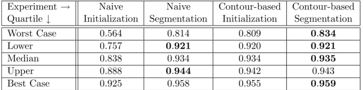
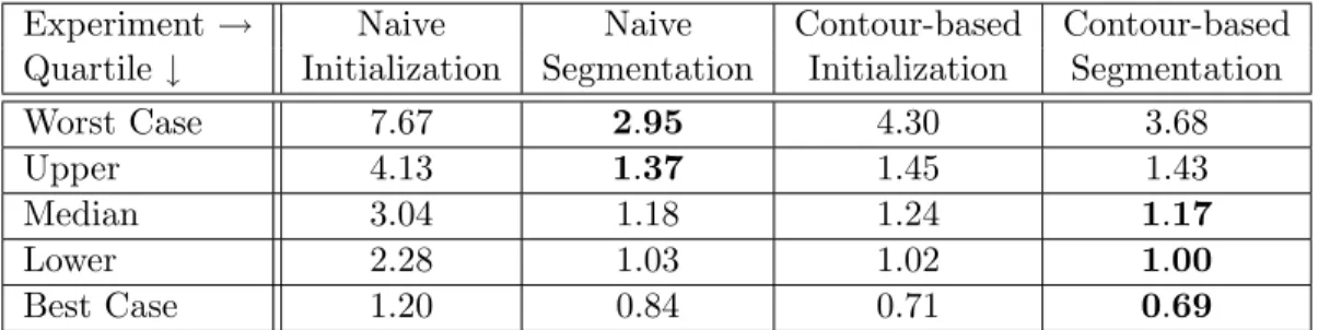
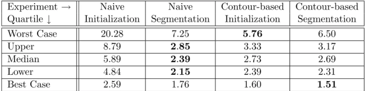
3.1 Evaluation of bladder initializations and segmentations . . . 87 3.2 Dice similarity coefficient for bladder initializations and segmentations . . . 88 3.3 Average surface distance for bladder initializations and segmentations . . . 89 3.4 90% worst surface distance for bladder initializations and segmentations . . . . 89 3.5 Evaluation of bladder initializations and segmentations . . . 94 3.6 Dice similarity coefficient for bladder initializations and segmentations . . . 95 3.7 Average surface distance for bladder initializations and segmentations . . . 95 3.8 90% worst surface distance for bladder initializations and segmentations . . . . 96 3.9 Dice coefficient after restricting P to an edge in the image . . . 97

(8)

LIST OF FIGURES

1.1 Examples of medical images . . . 1

2.1 Gaussian probability density functions . . . 18

2.2 Principal component analysis of a toy data set . . . 23

2.3 Medial geometry . . . 26

2.4 Classification of points on the medial locus . . . 27

2.5 Implicit shape representations . . . 35

2.6 The linear average of two signed distance maps . . . 38

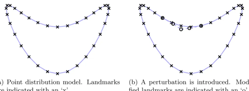
2.7 Point distribution model . . . 40

2.8 Perturbation of a point distribution model . . . 44

2.9 Histograms and quantile functions . . . 56

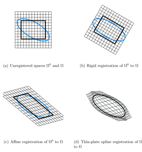
2.10 Registration . . . 64

3.1 CT image of the male pelvis . . . 77

3.2 Loose axial correspondence . . . 83

3.3 Pelvic scale alignment of bladder segmentations . . . 99

3.4 Dice similarity coefficient of bladder initializations and segmentation . . . 100

3.5 Average surface distance of bladder initializations and segmentation . . . 100

3.6 90% worst surface distance of bladder initializations and segmentation . . . 101

3.7 Multi-patient alignment of bladder segmentations . . . 102

3.8 Dice similarity coefficient of bladder initializations and segmentation . . . 103

3.9 Average surface distance of bladder initializations and segmentation . . . 103

3.10 90% worst surface distance of bladder initializations and segmentation . . . 104

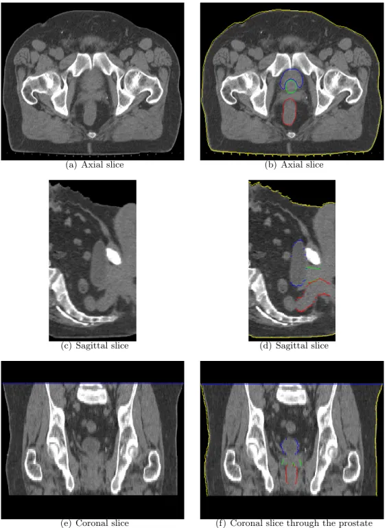
4.1 Axial slice of a CT image and prostate segmentation . . . 111

4.2 Non-credible regions on a bladder segmentation . . . 113

4.3 Non-credible regions on a prostate segmentation . . . 114

4.4 Image acquisition errors produce false-positive non-credible regions . . . 115

4.5 A display showing multiple degrees of non-credibilty for a blad-der segmentation . . . 116

4.6 Distribution of errors for a population of bladder and prostate segmentations. . 117

4.7 Distribution of RIQF-based image match values for bladder and prostate segmentations . . . 118

4.8 ROC analysis of the tests of segmentation non-credibility . . . 120

5.1 Rotational-flows interpolation in two dimensions. . . 128

5.2 Resumption of an interrupted interpolation . . . 130

5.3 Centers of rotation for rotational-flows interpolation of similar curves . . . 132

5.4 Three-dimensional rotational-flows interpolation . . . 135

5.5 Rotational-flows interpolation between similar shapes in 2D . . . 138

5.6 Rotational-flows interpolation between non-similar shapes in 2D . . . 139

(9)

5.8 3D rotational-flows interpolation between similar shapes . . . 143

5.9 Fractional anisotropy of transformations produced by rotational-flows interpolation of similar surfaces . . . 144

5.10 Comparison of fractional anisotropy of transformations pro-duced by linear and rotational-flows interpolations . . . 145

5.11 3D rotational-flows interpolation between non-similar shapes . . . 146

5.12 Fractional anisotropy of transformations produced by rotational-flows interpolation of non-similar shapes . . . 147

5.13 Rotational-flows interpolation of m-rep lung models . . . 148

5.14 Computation of a mean blader via convex combinations . . . 152

5.15 The mean bladder produced via convex combinations . . . 153

5.16 Riemannian interpolation of misaligned shapes . . . 153

(10)

LIST OF ABBREVIATIONS

ART adaptive radiotherapy

ASM active shape model

CDF cumulative density function

CT computed tomography

DVH dose-volume histogram

DRIQF discrete regional intensity quantile functions HDLSS high dimension, low sample size

IID independent and identically distributed MAP maximum a postoriestimation

MLE maximum likelihood estimation

MR magnetic resonance

PCA principal component analysis PDM point distribution model PGA principal geodesic analysis

QF quantile function

RIQF regional intensity quantile functions ROC receiver operating characteristic

RT radiotherapy

SDM signed distance map

(11)

Chapter 1 Introduction

1.1 Motivation: Object-Based Medical Image Segmentation

The use of medical images to guide diagnostics, therapies, and therapy-evaluations is im-proving the clinical outcome and quality of life for patients with a variety of conditions. In these situations the clinician must understand the images in order to treat the patient.

Fig. 1.1 shows examples of medical images. The left pane is an X-ray image showing a severely fractured femur [1]. This image is fairly easy to understand. The bone is the bright object in the foreground and the fracture is the large-scale discontinuity in it. The right pane is the mid-sagittal slice of a computed tomography (CT) image of the male pelvis. Locating the prostate and bladder (green and cyan outlines, respectively) in this image is a challenging task.

Figure 1.1: Examples of medical images

(12)

tosegment the image. Heresegmentationrefers to the process of assigning labels to the voxels of the image that belong to an object or structure of interest. Once the image has been segmented the end users can easily understand it in the context of the specific medical task at hand via a casual glance at its label-map. However segmentation itself can be a difficult and time consuming task.

Segmentation methods are characterized in the following three ways based on the level of control the user has over the segmentation. Manualsegmentation methods give the user the flexibility to control the labeling of each voxel, although they may feature tools that allow the user to assign a label to a region larger than a single voxel. Semi-automatic segmentations rely on limited user interaction in conjunction with automated image processing in order to label the image voxels. Automatic segmentation methods assign labels to voxels entirely on the basis of computerized image processing without any human interaction at all.

Automatic and semi-automatic segmentation methods are desirable for several reasons. The time and attention of the clinician is a scarce resource, whereas computational cycles are a commodity. If the medical expert can be relieved of the burden of producing segmentations, she can reallocate that time to better serve her patients. Furthermore, computers can pro-duce reproducible segmentations, but human experts are subject to intra- and inter- human variabilities.

A powerful subclass of (semi-) automatic methods are those that are object-based. These methods are programmed to understand the geometry of an object (or structure) of interest. The set of voxels assigned the label for that object will have geometry that is consistent with the object itself. An object-based segmentation method that follows Bayes’ rule for posterior optimization is a principled way to mimic manual segmentations. If the target object is the prostate, Bayes’ rule instructs the computer to find a prostate-shaped object with prostate-like intensity patterns in and around it in the image. The “prostate” label is assigned to the voxels in the interior of that object.

(13)

prob-ability distributions are generalizable if a novel object, or image intensity pattern relative to the object, from the target population is admitted with a high probability. These probabil-ity distributions are specific if all shape instances (resp. image patterns) that are admitted with high probability are representative of the target population. High generalizability and specificity are both desirable properties for the probability distributions used during Bayesian segmentation.

Returning to the example of prostate segmentation, a shape prior with high specificity gives the end user confidence that the final result will be “prostate-shaped”. A highly generalizable shape prior gives the user further confidence that a suitably large space of “prostate-shaped” objects will have been examined. A data likelihood with high generalizability allows the user to believe that the target object will be recognized as having an appropriate intensity pattern. When the data likelihood is also highly specific, it becomes less likely that the segmentation will converge to a false optimum elsewhere in the image.

Bayesian segmentation methods should not be used when the shape prior and data like-lihood distributions cannot be learned. For example, when working with CT images of the head and neck, regions of the lymphatic system cannot be seen directly. They are understood implicitly based on known relationships to nearby structures such as muscles, glands, blood vessels, and bones. In this application a segmentation method that transfers labels from a manually segmented atlas imageto the target image is more appropriate. This transfer func-tion is often defined by producing a warp of the ambient space that minimizes an energy function on the warp and the difference between the atlas image and the warped target image. I use the termatlas-based segmentation to refer to this method of producing a warp in order to transfer labels from the voxels of the atlas.

If an atlas-based segmentation method is forced to conform to object-based segmentation for the subset of targets that have already been well segmented, the segmentation of the entire complex of targets will be more relevant. This is true because errors involving that subset of pre-segmented targets will be bounded by the object-based segmentation and because the locations of these objects constrain the possible locations of the others.

(14)

segmen-tations are successful and that the atlas-based segmensegmen-tations will adhere to those object-based segmentations. In this dissertation I address those assumptions with an initialization strategy that produces high-quality object-based segmentations, with a statistical test that allows the clinician to be confident in the quality of the object-based segmentations she uses, and with a geometric tool for warping between object instances that can be used to drive a diffeomorphic warp between an atlas and a target image.

1.2 Semi-automatic Segmentation Initialization via a Sparse

Set of Contours

A known limitation of object-based segmentation methods is that they frequently are equiv-alent to the optimization of a non-convex objective function and are susceptible to local optima problems. It is generally assumed that the objective function has its global optimum at the de-sired answer and that in some local neighborhood around that answer there are no other local optima. When such an object-based segmentation is initialized with a shape instance that is outside of this neighborhood, there is a risk that the method will hallucinate a segmentation in some other region of the image that happens to be locally optimal. An initialization strategy that begins the optimization within the capture range of the global optimum mitigates this risk.

One would expect that when the segmentation routine is seeded with an initial shape that is in the correct image region the final segmentation result will also be in that region. Although this assumption typically is correct, it does not produce a practical solution as it requires a segmentation of the target image in order to produce the initial shape instance that is used to segment the target image. However, in the setting of Bayesian segmentation, a shape prior with high generalizability can be used to produce a shape instance that is close to the desired answer without requiring a full segmentation of the target image.

(15)

selected points.

The goodess of fit of this approximated shape typically increases with the number of man-ually specified points. But, because the user’s time and attention are scarce resources, it is important to limit the number of points the user is asked to identified. However, when too few points are specified, this approximated shape is likely to be inadequate and the final seg-mentation is likely to not be clinically usable. Consequently, the cost of manually correcting erroneous segmentations must also be taken into account when specifying the points the user is to identify at initialization time.

I propose a strategy for approximating a bladder segmentation from a subset of the bound-ary points found on only three axial slices of a CT image. A shape prior trained on bladder segmentations is used to find a bladder shaped object with boundary points near the ones identified on the three image slices. This shape model is suitable to initialize an object-based segmentation of the bladder that typically needs little or no manual correction to be clinically usable. Initialization strategies for the prostate and rectum are also discussed in this chapter, as is an alternative semi-automatic segmentation procedure that refines this approximated ob-ject by first having the user adjust the boundary and then generating a new candidate obob-ject from the shape prior that is matched to the modified boundary points.

1.3 Estimating the Local Credibility of a Segmentation

(16)

corruption can occur even if the failure is localized to a small region in the image.

Perhaps the safest behavior would be to have a trained expert, or better yet a team of trained experts, carefully review the validity of every segmentation produced. Unfortunately the scarcity of these experts and the fact that their time and attention can not possibly scale with number of images in need of analysis makes this option unfeasible.

Just as computerized segmentation methods are expanding the number of medical images that users can segment, computerized validation methods are needed to expand the number of segmentations that users can validate. The relationship between correct segmentations and the associated image intensity patterns captured by a Bayesian data likelihood distribution can be an important tool validating the segmentation of a new target image. If the image intensity pattern in and around the segmentation of the target image is inconsistent with what is known from the data likelihood distribution, further validation of the segmentation is warranted.

A mathematical function that can be used to evaluate the data likelihood for a new seg-mentation is often known as ageometry-to-image match function or simply as animage match

function. When an image-match function can be decomposed into independent terms for different regions of the segmentation or its boundary, each such term is known as a local

(geometry-to-) image match function.

In Chapter 4, I present a method that identifies statistical outliers of local geometry to image match functions asnon-credibleregions where the user should concentrate her validation efforts. This method has been applied to segmentations of the bladder and prostate from CT, and the identified non-credible regions were correlated with large disparities between the segmentations being tested and reference manual segmentations of the same images.

(17)

be corrected. In this case, pushing the boundary further outward is likely to produce the desired segmentation.

By applying the tests described in Chapter 4, the end user can increase her confidence in the quality of a given segmentation, and she can manually correct it when needed to produce a medically relevant segmentation.

1.4 Interpolation of Oriented Geometric Objects via Rotational

Flows

The tools proposed in Chapters 3 and 4 allow a medical user to produce an object-based segmentation of an appropriate target structure and to become confident in the quality of the segmentation before using it.

One possible application for high quality object-based segmentations is to provide a means for segmenting other structures that are not amenable to object-based methods. Suppose the user has an atlas image in which a variety of structures have been labeled. Assume that object-based segmentations are feasible for some, but not all, of the labeled structures in the atlas. The transformation that brings an object (or set of objects) from a configuration that segments the atlas into a configuration that segments the target image, could be extrapolated to define a mapping from the atlas image volume to the target image volume. This mapping when applied to the segmentation of one of the other structures in the atlas produces a segmentation of that structure in the target image.

(18)

suitable initialization for object-based segmentation of the intermediate image.

In Chapter 5, I present a novel method for interpolating between two objects. The in-terpolation produced by this method can be used to describe the transformation between an object in the atlas and an object in the target image. A sampling of boundary points on these interpolated objects can serve the landmark paths which are commonly used to define mappings between images. The interpolation can also be used to produce intermediate objects to initialize object-based segmentations for a time series of images.

This interpolation method is based upon a concept that I call rotational flows. The in-terpolation requires correspondence between samples of the initial and target objects as well as a complete frame to orient each sample. The rotational flows cause each sample to move along a circular arc, rotating about a uniquely determinedrotational center so that the angle swept out by the arc matches rotation needed to transform the reference frame into its target configuration.

Because rotational-flows interpolation connects position with orientation, it tends to be more shape maintaining than methods that interpolate those two independently. Specifically when the atlas and target objects are related by a similarity transformation, all interpolated objects are also similar to the reference set. When the transformation from the atlas to target object requires a shape change, the method of rotational flows frequently produces a visually satisfying interpolation.

1.5 Thesis and Contributions

(19)

interpolations from atlas object instances to credible segmentations produce a set of landmark paths that can be used in the large-scale diffeomorphism framework to map the full set of labels on the atlas to the target image.

The contributions of this dissertation are as follows:

1. Evidence that given a shape prior with adequately high generalizability and specificity, a dense object boundary can be recovered from a sparse sampling of boundary points.

2. Strategies for how a user can simply produce such a boundary sampling to recover a shape model for the bladder from easily identifiable points found on relatively few CT image slices.

3. Applications of this recovered shape to initialize or refine a semi-automatic segmentation.

4. A novel tool that identifies statistical outliers of a localized geometry-to-image-match function as regions where a segmentation is not credible.

5. A novel method for shape interpolation that synchronizes local changes of position and orientation. This method is driven by “rotational flows” about “rotational centers”

6. A method for computing the mean of a shape population based on pairwise interpolations via the method of rotational flows.

1.6 Overview of Chapters

(20)

(21)

Chapter 2 Background

Image analysis algorithms can be classified as low-levelmethods that simulate how the hu-man visual system responds to signals in the images, such as detectors for edges [10] and other image features [28, 53], and high-level methods that provide greater abstraction to perform more complicated tasks, such as the segmentation, tracking, and recognition of objects. High-level methods are often built by combining low-High-level feature detectors with other constraints based on the physics or geometry [42, 36] of a target object, or the statistics of a population of objects [19, 26].

Medical image segmentation is an important tool for helping clinicians and researchers to use images to understand the anatomy of a patient or subject. In this chapter I survey high-level methods for segmenting medical images and metrics for evaluating segmentation quality.

2.1 Medical Image Segmentation

Throughout this dissertation I will use following notation. Let Ω denote an imaging target. To simplify notation I will assume that

Ω ⊂ _R3_, _(2.1)

(22)

one- and two-dimensional images, and a time series of three-dimensional images can be thought of as a single four-dimensional image.

An image, denoted by

−I, is a map

−I : Ω → V (2.2)

whereV is the image value. For many medical imaging modalities the image has scalar values:

V ⊂R. (2.3)

As an example, the value of each voxel in a CT image is the average linear attenuation co-efficient for the material in that volume and describes the density of that material. Images that assign a tuple of values to each voxel are used in medicine as well. For example, diffusion tensor magnetic resonance (MR) imaging takes a scalar measurement from each of a set of magnetic gradient directions to produce a multiple values for each voxel. However, I will make the simplifying assumption that

−I is scalar-valued.

LetL denote a label and letSL denote the segmentation ofL for₋I.

SL ⊂ Ω (2.4)

is the set of voxels for which L is an appropriate label. The label L may identify an organ, such as the kidney, or a tissue class, such as white matter in the brain. In those examples, the segmentationSL would be the subset of voxels in the image that correspond to the kidney or

to white matter. In many segmentation applications, only a single label L is of interest. To simplify notation in such cases, the indexL will be omitted, andS will be used to denote the segmentation.

A manual segmentation process requires a human with domain knowledge to identify the voxels in SL. This human is often known as the rater. In a semi-automatic segmentation

process the computer identifiesSLwith limited human interaction, and in a (fully-) automatic

(23)

Segmentation methods that are (semi-) automatic have several potential advantages over manual processes. Manual segmentation of medical images can be a time consuming process, but (semi-) automatic segmentation can be much faster. In a clinical setting this speed-up could allow medical professionals to reallocate time spent manually segmenting images to other aspects of patient care. It could also reduce the time between image acquisition and the treatment of a patient. In some applications, the snapshot of the patient’s anatomy in the image is only relevant for a limited time. In these cases, a fast computer-generated segmentation may mean the difference between having a clinically usable image or not.

The speed advantage of (semi-) automatic segmentation is important in a research setting as well. It can allow researchers to study a larger data set in a fixed time frame than would be possible with manual segmentations. It can allow researchers to produce their results faster. Computerized segmentation methods are typically able to scale with the number of images to be studied, so it can be relatively easy and inexpensive for researchers in a retrospective study to reduce their image processing time by purchasing more computers. In contrast, if the same researchers relied on manual segmentations, hiring additional raters is likely to be difficult and expensive. Even if the study can afford and has access to additional raters, inter-rater variability can lead the researchers to false conclusions.

Computer-generated segmentations can offer greater reproducibility than a manual pro-cess. Given a fixed input, a deterministic method will always produce the same segmentation. However multiple manual segmentations of an image will be subject to inter- and intra-rater variabilities.

Inter-rater variability is known to be quite large [44, 52, 79]. Different institutions may have different protocols for segmenting the same objects, leading to gross differences when two raters segment the same image. Even when the raters follow the same protocol, they may exhibit systematic biases based on their training.

Intra-rater variability is also known to be a significant issue [79, 76] due to the following factors. It can be difficult for the rater to see the boundary between SL and Ω SL in

(24)

the rater. In three-dimensions, the rater typically produces the segmentation by examining two-dimensional slices of the image. It is difficult for the rater to produce a segmentation that is consistent across slices. The quality of the segmentation is also dependent on amount of time the rater can devote to it and will be negatively affected if the rater is distracted or interrupted.

Because of the reproducibility and speed advantages that computerized segmentation meth-ods hold over manual segmentations, a successful automatic segmentation method will be of great value to clinicians and researchers alike. The most general methods for segmenting im-ages rely only on the image intensities and assign the same label to a set of nearby-voxels with similar values [91], with different labels on opposite sides of a boundary in the image. However, there are many applications where these methods fail due to a lack of strong intensity differences between nearby structures of interest. For example, assigning separate labels to the bladder and prostate in a (non-contrast enhanced) CT image of the male pelvis is difficult because there is very little change in appearance between the two objects.

In these challenging cases a segmentation method that is tailored to the specific target labels has the potential for greater success. The geometric relationships between the targets and between each target and other nearby structures are valuable information that can be used at segmentation time. Using the male pelvis as an example, a segmentation method that incorporates a priori models of what it means to be bladder-shaped or prostate-shaped, of the relative positioning of the two organs, and of their positions relative to the pubic bones and the rectum is likely to produce better segmentations of those organs than a segmentation method that relies on image intensity alone.

Object-based segmentation methods are a class of segmentation methods that adjust an

a priori geometric model, denoted by m₌_L, to match the target L in the image data. The segmentation SL is the set of voxels on the interior of m=L. I discuss the theory of

(25)

2.2 Object-Based Segmentation

Many object-based segmentation methods have been proposed in the literature, including the methods described in [12, 18, 42, 43, 65, 82]. All of these methods segment a novel image, which I will denote by

−I, by adjustingm=L so that it bests matches the image data subject to

method-specific constraints. Thus object-based segmentation is an optimization problem.

There are two common formulations for this optimization problem. It may be posed as an

energy-minimizationproblem,

=

m_L = arg min =

m C m=

(2.5)

C(·) ≥ 0.

The functionC m₌

is the cost, or energy level, associated with that configuration of the model. Typically this cost function includes a term based on how well the model is supported by the image data and a term based on the geometry of the model in this configuration. Specific examples ofC(·) are given in Section 2.5.1 and Section 2.5.4.

Segmentation can also be posed as a statistical estimation problem.

=

m_L = arg max =

m p

−I|m=

(2.6)

or

=

m_L = arg max =

m p

=

m|

−I

(2.7)

The optimization (2.6) is known as maximum likelihood estimation (MLE), as the likelihood of the model given the image is being maximized. The optimization (2.7) is known as maximum

a postori estimation (MAP), as it is the posterior probability of the model conditioned on the image that is being maximized.

The likelihood function, p

−I|m=

, is typically learned from a set of training of exemplars. This function is minimized directly to produce an MLE segmentation. p

−I|m=

(26)

of Bayes’ Rule.

pm₌|

−I

=

p −I|m=

·p m₌

p −I

, (2.8)

wherep m₌is known as the prior distribution on the model. This probability distribution can be learned from training data. Specific examples of p

−I|m=

and p m₌ are given in Section 2.5.2 and Section 2.5.3.

Substituting (2.8) into (2.7), we see that for MAP estimation

=

m_L = arg max =

m

p

−I|m=

·p m₌

p

−I

= arg max =

m p

−I|m=

·p m₌

(2.9)

because p

−I

can be assumed to be constant for the image that is being segmented, even as

=

m varies.

There is a relationship between the energy-minimizing and probability-maximizing forms of segmentation. A cost function can be transformed into a probability by assuming an expo-nential distribution on the cost and then setting

p(·) ∝ exp (−C(·)) (2.10)

Because we are interested in the maximizer of the probability distribution rather than the distribution itself, we need not solve for the exact scalar factor that relatesp(·) to exp (−C(·)).

(27)

the probability density function.

C m₌ = −log

p

−I|m=

(2.11)

or

C m₌

= −logp −I|m=

−log p m₌

(2.12)

where (2.11) applies to the MLE framework and (2.12) applies to the MAP framework. This conversion is especially useful when the probability distributions in question are Gaussian.

The statistics of multivariate Gaussian distributions are reviewed in 2.3. When data can be assumed to follow a multivariate Gaussain probability distribution, the parameters of that distribution can be learned via principal component analysis (PCA). PCA is discussed in greater detail in Section 2.3.1 and is an important statistical tool used by many of the object-based segmentation methods surveyed in Section 2.5. The -log probability terms of (2.11) and (2.12) can be understood as measures of distance from the mean of a population and can be expressed in a simple form for Gaussian data in general and with respect to PCA in particular.

2.3 Statistics of Multivariate Gaussians

Suppose that

−

x is an n-vector drawn from the multivariate Gaussian distribution. By definition, for any vector of coefficients

−

a, the linear combination

−a·−x is normally distributed.

The notation

−

x ∼ N(µ,Σ) (2.13)

indicates

−

x is drawn from a Gaussian distribution that has a mean

−

µand non-singular covari-ance matrix Σ. The probability density function for this distribution is

p − x = 1

(2π)n2 √

det Σexp

−1 2 − x− − µ T

Σ−1

− x− − µ (2.14)

(28)

(a) In 1 dimension, with varying Σ (b) In 1 dimension, with varyingµ

(c) In 2 dimensions, with isotropic Σ (d) In 2 dimensions, with anisotropic Σ

Figure 2.1: Gaussian probability density functions.

Suppose

−v is a constant n-vector and A is a constant m×nmatrix. The effects of linear

transformations of

−

x are as follows.

−x+−v ∼ N

− µ+

−v,Σ

(2.15)

A −

x ∼ N

A

−

µ, AΣAT

(2.16)

The function −logp −

(29)

Mahalanobis distance, which is denoted byd_mahal

− x

and is defined in (2.18).

−log p −x = log

(2π)n2 √ det Σ +1 2

−x−₋µ

T

Σ−1

− x− − µ (2.17) d_mahal − x = s − x− −µ T

Σ−1

− x− − µ (2.18) d_mahal −x 2 = − x− −

µTΣ−1

− x−

−

µ (2.19)

= 2 −log p −x

−c (2.20)

c in (2.20) refers to the term in (2.17) that does not involve

− x.

The Mahalanobis distance is a statistical tool for measuring the distance from a sample to a population mean. It accounts for the anisotropy and orientation of the population’s distribu-tion. The Mahalanobis distance is easy to calculate and has a straightforward interpretation in applications of principal component analysis (PCA).

2.3.1 Principal Component Analysis

PCA can be used as a tool for learning a probability distribution from a set of training exemplars. When the data are assumed to be drawn from a multivariate Gaussian distribution, PCA projects the data onto a set of orthogonal bases such that the projection coefficients are standard (zero mean, unit variance) independent univariate Gaussian random variables.

This formulation is useful in a generative setting, as independent samples from a standard univariate Gaussian distribution can be combined to create new data instances. It is also useful in a discriminative setting where the Mahalanobis distance is a natural measure on the data.

Suppose

=

x =

−x1 ... −xk

(2.21)

is a set of ksamples and that each sample

−xi is written as an nelement column vector. The

(30)

The first step in PCA is to center the data and compute its n×n covariance matrix.

Let

−µ = meani=1..k

− xi

(2.22)

− x0_i ←

−xi−₋µ (2.23)

Σ = 1

k−1 x=

0

=

x0T (2.24)

The covariance matrix is known to be symmetric:

Σi,j = Σj,i ∀i, j, (2.25)

and positive semi-definite:

−aTΣ−a ≥ 0 ∀−a. (2.26)

From these two properties it follows that singular value decomposition on Σ will yield its eigenvectors and eigenvalues.

Σ = VΛVT , where (2.27)

Λi,i = λi (2.28)

Λi,j6=i = 0 (2.29)

ΣV·,j = λjV·,j (2.30)

VTV = Idn (2.31)

The matrix Λ in (2.27) is the diagonal matrix of the eigenvalues of Σ. The matrix Idnin (2.31)

is the n×n identity matrix. As a convention, the eigenvalues of Σ are sorted in descending order.

(31)

A sample

−x∼N

− µ,Σ

can be rewritten as follows.

− x= − µ+ − x− −

µ (2.33)

− x=

− µ+Pn

i=1

− x−

− µ·V·,i

V·,i (2.34)

− x=

− µ+Pn

i=1 „„

−x−−µ

«

·V·,i

«

√

λi

√

λiV·,i (2.35)

Each coefficient of the form „„

−x−−µ

«

·V·,i

«

√

λi in (2.35) can be shown to be an independent and

identically distributed (IID) standard normal random variable by (2.15) and (2.16).

− x−

−

µ ∼ N(µ−µ,Σ) (2.36)

∼ N(0n,Σ) (2.37)

V·,i

√ λi T − x− −µ

∼ N 0,√V·,i

λi

T Σ√V·,i

λi

!

(2.38)

∼ N

0, 1 λi

V_·T_,iΣV·,i

(2.39)

∼ N

0, 1 λi

V_·T_,iVΛVTV·,i

(2.40)

∼ N

0, 1 λi

λi

(2.41)

∼ N(0,1) (2.42)

This leads to the following expression for

d_mahal − x 2 : d_mahal − x 2 = n X i=1 − x− − µ·V·,i

2

λi

. (2.43)

Equation (2.35) also leads to an algorithm for generating new data instances according to the learned distribution. Let

−

αbe anntuple of IID standard normals. A new data instance

(32)

be generated by

−a = ₋µ+

n

X

i=1

αi

p

λiV·,i. (2.44)

Its squared Mahalanobis distance is merely

d_mahal −a 2 = n X i=1

αi2 . (2.45)

PCA For Dimensionality Reduction and Robust Estimation

Equations (2.35) and (2.44) assume that allneigenvalues of Σ are non-zero and are retained by the PCA. In practice this is typically an unworkable approximation.

Many applications in medical image analysis suffer from the high dimension, low sample size (HDLSS) problem. Because the cost of training exemplars is frequently high and because data representations for shape models and images can require hundreds, millions, or more features, the number of samples kn. In this case rank (Σ)≤(k−1). Thus, Σ has at most (k−1) non-zero eigenvalues. Even when HDLSS is not a problem, correlations in the data may mean that it actually lies in anm < ndimensional subspace.

When only the first m eigenvalues of Σ are non-zero, rewriting (2.35) as

− x=

−µ+

Pm

i=1 „„

−x−₋µ

«

·V·,i

«

√

λi

√

λiV·,i (2.46)

reduces the dimensionality of the data fromntom, as each sample can represented by its m

coefficients of the non-zero eigenvectors.

Projection of a sample onto the first meigenvectors:

−

x≈ Proj_m

− x=

− µ+Pm

i=1 „„

−x−−µ

«

·V·,i

«

√

λi

√

λiV·,i (2.47)

(33)

V·,1 = arg max

−v

var

− x0·

−v

(2.48)

V·,1 = arg min

−v

var

− x0−

− x0·

−v

(2.49)

V·,m = arg max

−v

var

−

x0−Proj_m−1

− x0 · −v (2.50)

V·,m = arg min

−v

var

−

x0−Proj_m−1

− x0 − − x0·

−v

(2.51)

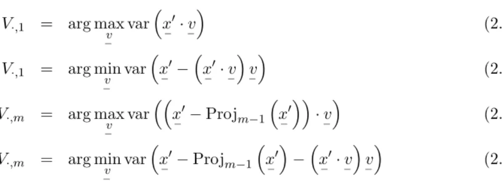
V·,1 is the direction that maximizes the variance of the projections of the centered data and minimizes the variance of the residuals. Likewise, the eigenvectors corresponding to the m

largest eigenvalues span the m-dimensional space that maximizes the variance of the projec-tions of the centered data and minimizes the variance of the residuals. Thus,

−

µplus the span of

V·,1...V·,m is the best mdimensional linear space for approximating the original training data.

The relationship between the data₌x and the eigenvectors of Σ is illustrated in Figure 2.2.

−2 0 2 −2 0 2 −2 0 2

(a) Points inR3

−2 0 2 −2 0 2 −2 0 2

(b) Projection onto the first prin-cipal component

(c) Projection onto the first two principal components

Figure 2.2: Principal component analysis of a toy data set. Figure 2.2(a) shows a scatter plot of points in 3 dimensions. Figure 2.2(b) adds a heavy line indicating the first principal component: the line formed by µ+αV1. The projections of the points onto this line are

shown with a thin red line. Figure 2.2(c) shows the points projected onto the first two principal components: the plane formed by µ+αV1+βV2.

Not only does PCA maximize the variance of Proj_m

−x

(34)

−x−Projm

− x

, but these variances are known.

var

Proj_m

− x

=

m

X

i=1

λ2_i (2.52)

var

−x−Projm

−

x =

n

X

i=m+1

λ2_i (2.53)

There are two commonly used strategies for choosing the number of eigenmodes to retain when using PCA for dimensionality reduction. One may choose an explicit threshold,, that all retained eigenvalues must be above.

m = arg max

m∗ (λm∗ ≥) (2.54)

Or one may choose to retain a variable number eigenmodes so long as a fixed percentageγ of the total variance is retained.

m = arg min

m∗

Pm∗

i=1λi

Pn

i=1λi

≥γ

(2.55)

There are computational and statistical benefits of using a reduced-dimensional PCA to learn the probability distributions optimized during a segmentation (2.11, 2.12). One compu-tational benefit of dimensionality reduction is that the storage requirement for the distribution scales with the number of eigenvectors that are retained. Another computational benefit is that the Mahalanobis distance for a data object can be used as a surrogate for its log proba-bility. The cost of computing the Mahalanobis distance scales withm. This is true whether the data object needs to be projected into the PCA space or the data is generated from the PCA by expanding a given set of coefficients (2.44). In this second case, the segmentation consists of optimizing over the set of coefficients. The size of the search space and the cost of the optimization increase with mas well.

(35)

typically performed on some artifact of a carefully drawn manual segmentation. These manual segmentations are very expensive, so it has become the norm to work with small datasets. Discarding the smallest eigenvectors from the PCA improves the overall robustness of the estimation of the probability distribution.

Because of this property of robustness against a limited sample size and because it allows computationally efficient methods for approximating the log probabilities needed to drive a segmentation, PCA is a popular tool for estimating the probability distributions used during object-based segmentation. Examples of its use will be given in Section 2.5. In some of these examples, the Mahalanobis distance is not used explicitly as a log probability calculation. Instead, the projection of a candidate object into the PCA space, and perhaps a truncation of the coefficients, will be used to constrain the optimization to lie in the learned shape space.

2.4 Medial Geometry

The segmentation method that I present in Section 2.5.3 uses medial descriptors as its shape representation. These medial descriptors provide a compact representation for an object m₌

and provide a coordinate system on the interior of m₌.

The medial axis of an objectm₌ was defined by Blum [5] as the locus of centers of maximal inscribed balls. Throughout this Section,

−p will denote a point on the medial axis of m= and

B

−p

will denote the maximal inscribed ball of m₌ that is centered at

−p. By definition, an

inscribed ball must lie on the interior of the object. To be maximal, it must not be contained in any other inscribed ball:

B

−p

⊂ m₌ (2.56)

B

−p

⊂ B0 → B0 6⊂ =

m,∀balls B0. (2.57)

An example object and its medial axis are shown in Figure 2.3

(36)

(a) The highlighted point on the medial axis is the center of a maximal inscribed ball. The ball is drawn with the two spoke vec-tors which point to the contact points on the object boundary.

(b) A point that is not on the medial axis is highlighted. The larger ball centered at this point is not inscribed as it crosses into the exterior or the object. The smaller ball is in-scribed in the object but is not maximal as it is a subset of another inscribed ball, which is also shown.

Figure 2.3: Medial geometry. An object boundary (black line) is shown with its medial axis (dashed line). A single point on the medial axis is highlighted in Figure 2.3(a). A point that is not on the medial axis is highlighted in Figure 2.3(b).

boundary ofm₌ to

−pvanish at the point of contact and that the (k+ 1)

th_{derivative is non-zero}

there. This contact is said to be of order k, and

−p is of type Ak. When

B

−p

makes order

k contact with m points on the boundary of m₌,

−p is said to be of type A

m

k. The catalog of

generically occurring points is quite small, and Giblin and Kimia have fully enumerated it.

The medial axis of a generic object in two dimensions will generically consist primarily of one or more curves of A2₁ points. If more than one such curve is present, the intersection of three curve segments at a point of A3₁ contact will generically occur. An A3₁ point can be understood as the coincidence ofA2

1 points from each of the three segments coinciding. Each of theseA2₁ points shares one of its contact points with the medial point from one of the other segments and shares its other contact point with the medial point from the third segment. Each end of a curve of A2₁ points will generically occur either at an A3₁ junction or at an A3 point. At the A3 point at the end of a segment of the medial axis, the two contact points collapse onto a single point that is an extremum of curvature on m₌, and

−p is the center of

(37)

(a) A two dimensional object and its medial axis.

(b) The medial axis of a three dimensional object.

Figure 2.4: Medial geometry. Generic contact points on medial axes are shown. These figures have been reproduced from [93] with permission from the author.

The medial axis of a generic object in R3 will generically consist of sheets ofA21 points as well as special curves at the boundaries and intersections of the sheets and special points at the intersections of the curves. Similarly to the two dimensional cases, three sheets of A2₁ points can join in a curve ofA3₁ points. Otherwise a sheet ofA2₁points will generically be bounded by a curve ofA3 points. The medial locus for a three dimensional object can generically include two contact types that are not seen for two dimensional objects. An A3₁ junction curve can intersect an A3 end curve at an A3A1 point. This happens when a sheet is attached to two others along part of its boundary, the A3A1 point is known as a “fin creation” point as it resembles a fin emerging from the body of a shark. Four A3

1 curves bounding six A21 sheets can generically intersect at a A4₁ point. An example of the medial locus for a generic three dimensional object and its contact types can be seen in Figure 2.4(b).

The catalog of contact-types is the basis for a strategy for understanding the object at a coarse scale. We can decomposem₌ ⊂_R3_{into components that correspond to distinct}_A2

1sheets on its medial axis. These sheets correspond to coarse scale structures inm₌. The connectiveA3₁

curves allow us to understand the relationships between these structures. Similarly m₌ ⊂R2

(38)

connections between them. I will use the notationM to refer to a curve or sheet ofA2₁ points.

TheA2

1 nature of points onM is instrumental in understanding how the medial axis can be found from the volume of an object. Suppose

−

p is of typeA2₁.

−

p is equidistant to two distinct nearest points on the boundary ofm₌ and must lie on its Voronoi diagram [45]. One method for finding the medial axis ofm₌ is to prune the Voronoi diagram for its boundary [80].

Consider the function d

=

m : Ω → R+, where dm₌

−x

is defined as the Euclidean distance from

−x to the nearest point on the boundary of m=. The value of d=m

−

p is equivalent to the radius of B

−

p. Since B

−

p is tangent to m₌ at the point of contact, they share the same normal direction. This direction can be found as the gradient of the distance map,i.e., ∇d

=

m.

The fact that B

−p

makes contact with two nearest points on the boundary of m₌ gives rise to the grass-fire [68] method for finding the medial axis. In this analogy suppose that the volume ofm₌ is full of evenly distributed prairie grass and that the grass at all boundary points is ignited simultaneously. The fire will burn inwards, along ∇d

=

m, at a constant speed. The

places where two fires quench each other are points on the medial locus. The time it takes for the fire to reach such a point is equivalent to the radius of the maximal inscribed ball at that point.

If the center and radius of each of the maximal inscribed balls is known, the boundary of m₌ can be reconstructed from an envelope around the balls. Each tuple of

− p, d = m − p is known as a order 0 medial atom. Although all information aboutm₌ is captured in its order 0 medial atoms, it is often convenient to have an explicit model of where B

−

pmakes contact with the boundary of m₌. An order 1 medial atom extends the order 0 medial atom with a pair of vectors from

−p to the points of contact. The collection of all order 1 medial atoms for

=

m are known as the m-repfor that object.

When the medial axis of an object inR2is decomposed into curves ofA21 points, the medial atoms on each curve can be understood as continuous functions of a single parameteru,e.g.,

normalized arc length along the curve. In this case the m-rep for the object is the set of medial atom functions from each A2₁ curve. Typical notation is to define the order 0 medial atoms with two continuous functions

−

X:{u} →R2 and r:{u} →R+ that give the central position

(39)

continuous functions

−

U+1 :{u} →_S1 _and

−

U−1 :{u} → _S1 _{that each give a unit vector in the} direction of a point of contact. That is, the contact points are at

−

X(u) +r(u)

−

U+1(u) and

−

X(u) +r(u)

−

U−1(u). Similarly the m-rep for an object in R3 can be understood as the set

of functions that produce medial atoms for each sheet of A2₁ points on the medial locus. Each sheet can be indexed by a pair of parameters denoted by the tuple

−u, and its medial atoms

can be understood as the following continuous functions:

− X :

n

−u o

→ R3, r : n

−u o

→ R+,

− U+1:n

−

uo→S2, and U₋−1 : n

−u o

→S2.

Damon [22] defined a generalization of a medial sheet known as a skeletal structure for an object. The skeletal structure consists of two-sided sets of points and their boundaries (i.e.,

curves and their end-points in R2 or sheets and their end-curves in R3). An outward vector

field that points to the boundary of the object is defined on each side of each set of points. Each of these vector fields is understood as the product of a scalar functionrand a unit vector field

−

U. It is clear that an m-rep that uses order 1 medial atoms fits the definition of a skeletal structure.

Thus far I have only discussed the transformation from a boundary representation of a shape into a medial representations. It is interesting to think about transformations in the other direction. One could define an arbitrary skeletal structure and think about the boundary it implies. Damon invented the radial shape operatorSrad to link the differential geometry of

a skeletal structure with the differential geometry of its implied boundary.

Srad is calculated locally for one side of the skeletal structure and separately for the other.

When computing Srad for a medial sheet M, U₋ can be assumed to consistently be chosen as

either

− U+1 or

−

U−1. The algorithm for computingSrad at for a medial atom onM follows.

Suppose

−v is a vector that is tangent to the medial sheet at ₋p: −v ∈ T −p

M. Srad is an

operator that takes

−vto the vector inT −p

that is opposite the projection along

−

U intoT −p

of the directional derivative of

−

U with respect to

−v:

(40)

SupposeX0 is the boundary point that corresponds to the medial atom at − X − u .

X0 =

− X

−

u+r −u − U −u (2.59)

WhenSrad atX₋

− u

is written in coordinates as a matrix, it can be related to the differential geometry shape operatorS atX0 as follows.

S =

Id−r

−u

Srad

−1

Srad , (2.60)

where Id is the identity matrix. From (2.60), Damon has shown that the eigenvalues of S: {κ1, κ2}, i.e., the principal curvatures of m= at X

0 _{have the following relationship with the}

eigenvalues ofSrad: {κr1, κr2}.

κi =

κri

1−r

− u

κri

i∈ {1,2} (2.61)

Becausem₌ will have a fold in it atX0 whenκi =∞ and becauseκri is a continuous function

for which 0 is a valid value, Damon is able to derive the compatibility condition (2.62) for legal boundaries from (2.61).

κri <

1

r − u

(2.62)

Srad is well defined for the A21 points on a medial sheet. Damon defined an analogous operatorSE, known as the radial edge operator that is valid at theA3 points on the boundary of a medial sheet. SE can be used to define compatibility conditions along that boundary.

It has been shown that an object m₌ that satisfies (2.62) everywhere along each medial sheet and thus has no folds in its surface will have the property that none of its medial atoms have crossing spoke vectors inside m₌. It follows that any point

−

x on the interior ofm₌ can be assigned unique coordinates in the following way. The first coordinate is used to identify a figure, i.e., to select a sheet of A2₁ points from the medial axis of m₌. The next coordinates,

(41)

τ : 0≤τ ≤1 identify a spoke vector and a fractional radius such that for some figure

−x = X−

− u

+τ r −u − Uφ − u . (2.63)

This object-relative coordinate system for the entire volume of the object is one of the impor-tant strengths of m-reps.

A weakness of the m-rep is that the number of medial sheets and the connections between medial sheets can be unstable with respect to relatively small surface deformations. Moreover, there may be medial atoms on a branching medial axis that have little information about the object boundary and only seem to exist to allow the medial axis to continue to a more salient location. Blum labels such medial atom as “ligature”. The sampled m-rep, which henceforth will be abbreviated to m-rep1, offers many of the benefits of the continuous medial axis, such as the existence of Damon’s radial and edge shape operators and an object-relative coordinate system, but is explicitly designed to avoid the instability of the number and connectivity of me-dial sheets and to provide a compact representation where all atoms make salient contributions to the object boundary.

The m-rep consists of sheets of sampled order 1 medial atoms that are arranged on a curve for objects with (nearly) circular cross-section and in a lattice for more general objects. In the m-rep atoms at the end of each curve or lattice are not strictly medial atoms. Let

−

u0 denote the

−

u coordinate of an end atom. A3 edge points are approximated by a medial atom at an

A2₁ location that is augmented by another scalar function, η :

n

− u0

o

→_R+_. _η _{is known as the} elongation factor, and it implies another position on the boundary of m₌ at

− X0 − u0 = − X − u0 + η − u0 r − u0 2 − U+1 − u0 + − U−1

− u0

(2.64)

The outward normal direction tom₌ at

− X0

−

u0is given by the spoke bisector 1₂

− U+1

− u0+

− U−1

− u0.

The point − X0 −u

is an extremum of curvature on the boundary ofm₌, as is the place where an A3 point on a continuous medial locus makes contact with its boundary. It is a sample of

(42)

the crest curve on the boundary of m₌. The curve formed by interpolating between the three spoke-ends of an end-atom explains the portion of the boundary that would be implied by medial atoms that lie between that sampled medial atom and theA3₁ point on the blum medial locus. Although these end atoms are not strictly medial, they do meet Damon’s criteria for skeletal structures.

Han [37] has developed a method for interpolation between the relatively sparsely sampled medial atoms of an m-rep. This interpolation allows a parameterized m-rep to be recovered from the samples of an m-rep. This is useful for understanding the object-relative coordinate system for the entire object volume.

When an m-rep is formed from more than one sheet, the linkage is specified so that atoms of one medial sheet, known as the subfigure, are placed at specified boundary positions on another figure, known as the host. A set of parameters define a new surface that blends between the boundaries implied by the host and subfigure. The blending algorithm and its parameters are described in greater detail in Han’s doctoral dissertation [35]. In short, the connection can be understood as a generalization of a skeletal structure in which the two sides of the hubs on the skeletal structure pull away from each other. A one-sided skeletal curve splits off from the medial axis of the host figure and approximates a ligature section of the subfigure. This one-sided skeletal curve ends at a place where it meets the traditional medial axis for the salient portion of the subfigure and another one-sided skeletal curve that approximates the “other” side of the medial axis in the ligature region. Han has been able to calculateSrad and evaluate

the compatibility condition for the one-sided skeletal structures, and thus he has been able to enforce geometric propriety in the blend region.

By construction, m-reps avoid changes to their meta-parameters: the number of medial lattices or curves, the connections between them, and the sampling of each. The m-rep instance for a new shape is produced by adjusting the atoms on a template m-rep to make its boundary best match the boundary of the target object. This depends of having access to an appropriate template m-rep.

(43)

a series of automatic [36] or manual edits, it can be made to match the target object.

Because of these advantages: its compact representation, the object-relative coordinate system for the object volume, the geometric benefits of Damon’s radial and edge shape oper-ators, and the stability of the subfigure sheets, m-reps are attractive for use in object-based segmentation. The details of m-rep-based segmentation are given in Section 2.5.3.

2.5 Popular Object- and Atlas- Based Segmentation Methods

I survey three popular object-based segmentation techniques: geodesic active contours [92, 12], the active shape model (ASM) and point distribution model (PDM) [19, 43, 88], and the deformable m-rep [65, 47, 50], in Sections 2.5.1 - 2.5.3 respectively. For each of these methods I describe the shape representation and its geometric constraints as well as the optimization method and its cost function or probability distribution(s).

The ASM and the m-rep can each be used to define a statistical deformable shape model (SDSM) for an object class. SDSMs are commonly evaluated based on their generalization ability: a measure of how well the SDSM can model a new instance of the same object class and based on their specificity: a measure of the extent to which objects generated by SDSM belong to the intended object class. Precise definitions of generalization ability and sensitivity are given by Styner et al. [81].

I discuss a fourth segmentation method: registration of an atlas image [16, 72, 41, 27], in Section 2.5.4. This method is not typically considered object-based, but there are opportunities for interaction between object-based and atlas-based segmentations that make it relevant to this dissertation.

2.5.1 Snakes, Geodesic Active Contours

(44)

to minimize is:

E_snake∗ =

Z 1

0

E_{int (}v(s)) +E_{image (}v(s)) +Econ (v(s))ds . (2.65)

The three terms in this energy functional E_int, E_{image, and} E_{con represent energies due}

to the internal bending of the spline, due to image forces, and due to external constraints respectively. The spline is evolved to a configuration that minimizes the energy functional for a given image.

The external constraint energyEcon in (2.65) provides a way for a user to steer the snake. A spring force can be used to penalize the snake for moving a specified point away from a designated location, and a repulsion force can be used to penalize the snake for moving towards a designated location. When these external constraints are specified, the snake produces a semi-automatic segmentation. The other two energies in (2.65), the internal spline state E_int

and the image energyE_{image, require no human input, and when they are used without}E_con

the snake produces a fully automatic segmentation.

During the 20 years since [42] was published, the snakes methodology has evolved into a widely used technology known as geodesic active contours [92, 12]. A change in the shape representation is one of the most important improvements of these newer methods over the original snakes.

In the geodesic active contours framework the shape model m₌_Lused to segment L in an

n-dimensional image is implicitly represented by the zero level set of a scalar-valued function on the imaging domain:

φ: Ω → _R, (2.66)

rather than by the explicit parameterization used in the original snakes. Typically the signed distance map (SDM) is used asφ[75]. Let

−

x∈Ω and let d −x

denote the distance from

(45)

the nearest point on the boundary implied by φ.

φ

− x

=



 

 

−d −x

,

−

x is on the interior of the object

d

−x

, −

x is on the exterior of the object

(2.67)

Negative distances in this map are associated with the interior of the object, positive distances are associated with the exterior, and the zero level set implies the boundary of the object. An example of this shape representation can be seen in Figure 2.5.

(a) The binary map for an object inR2

−5 0 5

(b) The signed distance map for this object

(c) The signed distance map interpreted as a height function inR3

Figure 2.5: Implicit shape representations.

This implicit shape representation has several useful properties. It allows the topology of

=

m_Lto change during the segmentation process. Such a change would not be possible with the original snake, or indeed with the ASM [19] or m-rep [36] shape representations discussed in Sections 2.5.2 and 2.5.3. This change in topology is desirable when the segmentation target is likely to have a different topology than the shape template, for example, when the segmentation target is in the presence of pathology. However, a change in topology is undesirable when the target has a known, fixed topology. Bai et. al [3] have demonstrated an extension of this method that is constrained to a fixed topology, but their constraint is computationally expensive.