S. Knight, I. Lanese, A. Lluch Lafuente and H. T. Vieira (Eds.): 8th Interaction and Concurrency Experience (ICE 2015) EPTCS 189, 2015, pp. 3–20, doi:10.4204/EPTCS.189.3
c
K. Dokter, S.-S. T. Q. Jongmans, F. Arbab & S. Bliudze This work is licensed under the
Creative Commons Attribution License. Kasper Dokter, Sung-Shik Jongmans, Farhad Arbab
Centrum Wiskunde & Informatica, Amsterdam, Netherlands
Simon Bliudze
´
Ecole Polytechnique F´ed´erale de Lausanne, Lausanne, Switzerland
Coordination languages simplify design and development of concurrent systems. Particularly, exoge-nous coordination languages, like BIP and Reo, enable system designers to express the interactions among components in a system explicitly. In this paper we establish a formal relation between BI(P) (i.e., BIP without the priority layer) and Reo, by defining transformations between their semantic models. We show that these transformations preserve all properties expressible in a common se-mantics. This formal relation comprises the basis for a solid comparison and consolidation of the fundamental coordination concepts behind these two languages. Moreover, this basis offers transla-tions that enable users of either language to benefit from the toolchains of the other.
1
Introduction
Context. Over the past decades, architecture description languages (ADL) and coordination languages have emerged as fundamental tools for tackling complexity in the design of correct-by-construction com-ponentised software systems [15]. However, no language has yet emerged as a de facto standard, and no consensus exists on how to properly design such languages, either. BIP [9, 10] and Reo [3] each addresses this complexity and provides a formal semantic framework, which allows reasoning about and proving correctness of coordination as a first-class entity.
BIP is a language for the construction of concurrent systems by superposing three layers: behaviour, interaction and priorities. The layered approach of BIP separates concerns between interaction and com-putation. This is essential for component-based design of concurrent systems, because it allows global analysis of the coordination layer and reusability of written code.
Reo is a language for compositional specification of coordination protocols, i.e., protocols modeling the synchronization and dataflow among multiple components. These protocols consist of graph-like structures, calledconnectors. Reo connectors may compose together to form more complex connectors, allowing reusability and compositional construction of coordination protocols.
We provide a more detailed introduction to BIP and Reo in Section 2.
Motivation. Both BIP and Reo advocate the necessity of separating coordination mechanisms from the coordinated components. In BIP one refers to this separation as thearchitecture-baseddesign approach [11]. Reo literature uses the termexogenous coordinationto describe the same fundamental principle [3, 4, 20]. Despite this fundamental agreement, the design choices underlying BIP and Reo differ. For example, BIP uses stateless interactions, while Reo allows stateful connectors. Establishing a formal relation between BIP and Reo is necessary to discover fundamental principles that drive the design of coordination languages.
Furthermore, establishing a formal relationship between BIP and Reo enables encodings that allow each of the two frameworks to benefit from tools and theoretical results obtained for the other. These toolchains include tools for editing, code generation, and model checking. We refer to [1] and [2, 4] for details.
Contributions. We relate the most important semantic models of BI(P)1 (i.e., BIP without the pri-ority layer) and Reo. For Reo we considerport automata andconstraint automata, which model Reo connectors at different levels of abstraction [16]. For BI(P) we considerBIP architectures[6] andBIP interaction models, i.e., sets of simple interaction expressions [11].
First, we provide a short summary of BIP and Reo in Section 2. Then, in Section 3, we define mappings between port automata and BIP architectures, and show that these distribute over composition modulo semantic equivalence. Hence, it is possible to compute these translations incrementally, in order to speed them up. In Section 4, we define mappings between stateless constraint automata and BIP interaction models. We show that all transformations preserve all properties of observable dataflow, which, for example, enables one to transfer safety properties established for some generated code, or the results of model checking from one model to the other. These mappings in the data-sensitive domain do not distribute over composition, but in Section 5 we briefly discuss a different translation scheme that still allows incremental translation. There, we discuss also the differences and similarities between BI(P) and Reo and other coordination languages, and point out future work.
Related Work. Other authors have related and compared both BIP and Reo to other coordination languages. Bruni et al. encode BIP models into Petri nets [12], and Chkouri et al. present a translation of AADL into BIP [13]. Proenc¸a and Clarke provide a detailed comparison between Orc and Reo [21]. Arbab et al. provide a translation of Reo connectors into the Tile Model [5]. Krause compared Reo to Petri nets [18]. Talcott, Sirjani and Ren connect both ARC and PBRD to Reo by providing mappings between their semantic models [22].
Although an indirect comparison of BIP and Reo through their respective comparisons with other models, e.g., Petri nets, is certainly possible, the direct and formal translations we present in this paper allows direct translation tools between BIP and Reo, that are otherwise difficult, if not impossible, to construct based on such indirect comparisons.
2
Overview of BIP and Reo
2.1 BIP
A BIP system consist of a superposition of three layers: Behaviour, Interaction, and Priority. The be-haviour layer encapsulates all computation, consisting ofatomic componentsprocessing sequential code.
Portsform the interface of a component through which it interacts with other components. BIP repre-sents these atomic components asLabeled Transition Systems(LTS) having transitions labeled with ports and extended with data stored in local variables. The second layer defines component coordination by means ofBIP interaction models [11]. For each interactionamong components in a BIP system, the interaction model of that system specifies the set of ports synchronized by that interaction and the way
sleep work
b1 f1
b1 f1
B1
sleep work
b2 f2
b2 f2
B2
(a)
f ree taken
b12 f12
b12 f12
C12
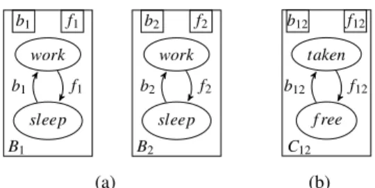
(b) Figure 1: BIP components (a); coordinator (b).
data is retrieved, filtered and updated in each of the participating components. In the third layer, priorities impose scheduling constraints to resolve conflicts in case alternative interactions are possible. In the rest of this paper, we disregard priorities and focus mainly on interaction models (cf., footnote 1).
Data-agnostic semantics. We first introduce a data-agnostic semantics for BIP.
Definition 1 (BIP component [6]). A BIP component C over a set of portsPC is a labeled transition system(Q,q0,PC,→)over the alphabet 2PC. IfC is a set of components, we say thatC isdisconnected iffPC∩PC0 =/0 for all distinctC,C0∈C. Furthermore, we definePC =SC∈CPC.
Then, BIP defines aninteraction modelover a set of portsPto be a set of subsets ofP. Interaction models are used to define synchronisations among components, which can be intuitively described as follows. Given a disconnected set of BIP componentsC and an interaction modelγ overPC, the state space of the corresponding composite componentγ(C) is the cross product of the state spaces of the
components inC;γ(C)can make a transition labelled by an interactionN∈γiff all the involved
com-ponents (those that have ports inN) can make the corresponding transitions. A straightforward formal presentation can be found in [10] (cf., Definition 3 below). Thus, BIP interaction models arestateless: every interaction inγis always allowed; it is enabled if all ports in the interaction are ready. However, [6]
shows the need for statefull interaction, which motivatesBIP architectures
Definition 2 (BIP architecture [6]). A BIP architectureis a tuple A= (C,PA,γ), where C is a finite
disconnected set ofcoordinatingBIP components,PAis a set of ports, such thatPC =
S
C∈CPC⊆PA, and
γ⊆2PA is adata-agnostic interaction model. We call ports inP
A\PC dangling portsofA.
Essentially, a BIP architecture is a structured way of combining an interaction modelγ with a set
of distinguished components, whose only purpose is to control which interactions inγare applicable at
which point in time (which depends on the states of the coordinating components).
Definition 3(BIP architecture application [6]). Let A= (C,PA,γ)be a BIP architecture, and Ba set
of components, such that B∪C is finite and disconnected, and that PA⊆PB∪PC. Write B∪C = {Bi |i∈I}, with Bi = (Qi,qi0,Pi,→i). Then, the application A(B) of A to B is the BIP component
(∏i∈IQi,(qi)i∈I,PB∪PC,→), where→is the smallest relation satisfying:(qi)i∈I N
−→(q0i)i∈I whenever
1. N=/0, and there exists ani∈Isuch thatqi /0 −
→iq0iandq0j=qj for all j∈I\ {i}; or
2. N∩PA∈γ, and for alli∈I we haveN∩Pi6=/0 impliesqi N∩Pi
−−−→iq0i, andN∩Pi=/0 impliesq0i=qi.
The applicationA(B), of a BIP architectureAto a set of BIP componentsB, enforces coordination constraints specified by that architecture on those components [6]. Theinterface PAofAcontains all ports
inB. In the applicationA(B), the ports belonging toPA can participate only in interactions defined by the interaction modelγ ofA. Ports that do not belong toPAare not restricted and can participate in any interaction.
Intuitively, an architecture can also be viewed as an incomplete system: the application of an archi-tecture consists in “attaching” its dangling ports to the operand components. The operational semantics is that of composing all components (operands and coordinators) with the interaction model as described in the previous paragraph. The intuition behind transitions labelled by /0 is that they representobservable idling(as opposed to internal transitions). This allows us to “desynchronise” combined architectures (see Definition 4) in a simple manner, since coordinators of one architecture can idle, while those of another performs a transition. Note that, ifN= /0, in item 2 of Definition 3,N∩Pi=/0, hence also,q0i=qi, for alli. Thus, intuitively, one can say that none of the components moves. Item 1, however, does allow one component to make a real move labelled by /0, if such a move exists. Thus, the transitions labelled by /0 interleave, reflecting the idea that in BIP synchronisation can happen only through ports.
Example 1(Mutual exclusion [6]). Consider the componentsB1andB2in Figure 1(a). In order to ensure mutual exclusion of theirworkstates, we apply the BIP architectureA12= ({C12},P12,γ12), whereC12is shown in Figure 1(b),P12={b1,b2,b12,f1,f2,f12}andγ12=
/0,{b1,b12},{b2,b12},{f1,f12},{f2,f12} . The interfaceP12ofA12covers all ports ofB1,B2andC12. Hence, the only possible interactions are those that explicitly belong toγ12. Assuming that the initial states ofB1andB2aresleep, and that ofC12is
free, neither of the two states (free,work,work) and(taken,work,work) is reachable, i.e. the mu-tual exclusion property(q16=work)∨(q26=work)—whereq1andq2 are state variables ofB1 andB2
respectively—holds inA12(B1,B2). 4
Definition 4(Composition of BIP architectures [6]). LetA1= (C1,P1,γ1)andA2= (C2,P2,γ2)be two BIP architectures. Recall that PCi =S
C∈CiPC, fori=1,2. IfPC1∩PC2 = /0, thenA1⊕A2 is given by
(C1∪C2,P1∪P2,γ12), whereγ12={N⊆P1∪P2|N∩Pi ∈γi,fori=1,2}. In other words,γ12 is the interaction model defined by the conjunction of the characteristic predicates ofγ1andγ2.
Data-aware semantics. Recently, the data-agnostic formalization of BIP interaction models was ex-tended with data transfer, using the notion ofinteraction expressions[11]. LetPbe a global set of ports. For each port p∈P, letxp:Dp be a typed variable used for the data exchange at that port. For a set of portsP⊆P, letXP= (xp)p∈P. An interaction expression models the effect of an interaction among ports in terms of the data exchanged through their corresponding variables.
Definition 5(Interaction expression [11]). Aninteraction expressionis an expression of the form
(P←Q).[g(XQ,XL): (XP,XL):=up(XQ,XL)//(XQ,XL):=dn(XP,XL)],
where P,Q⊆P are top and bottom sets of ports; L⊆P is a set of local variables; g(XQ,XL) is the boolean guard; up(XQ,XL) and dn(XP,XL) are respectively the up- and downward data transfer expressions.
For an interaction expressionαas above, we define bytop(α)=∆ P,bot(α)=∆ Qandsupp(α)=∆P∪Q
the sets of top, bottom and all ports inα, respectively. We denotegα,upα anddnα the guard, upward
and downward transfer corresponding expressions inα.
associated to the bottom ports satisfy a boolean condition. As a side effect, an interaction expression may also modify local variables inXL. Intuitively, such an interaction expression canfireonly if its guard is true. When it fires, its upstream transfer is computed first using the values offered by its participating BIP components. Then, the downstream transfer modifies all the port variables with updated values.
Definition 6(BIP interaction models [11]). A(data-aware) BIP interaction modelis a setΓofsimple BIP connectorsα, which are BIP interaction expressions of the form
({w} ←A).[g(XA): (xw,XL):=up(XA)//XA:=dn(xw,XL)],
wherew∈Pis a single top port,A⊆Pis a set of ports, such thatw6∈A, and neitherupnorginvolves local variables.
Example 2(Maximum). LetP={a,b,w,l}be a set of ports of type integer, i.e.,xp:Dp=Z, for all p∈P, and consider the interaction expression (simple BIP connector)
αmax= ({w} ← {a,b}).[tt: xl:=max(xa,xb)//xa,xb:=xl],
wherettis true. First, the connector takes the values presented at portsaandb. Then, the simple BIP connectorαmax computes atomically the maximum ofxa andxb and assigns it to its local variablexl. Finally,αmaxassigns atomically the value ofxl to bothxaandxb. 4
BIP interaction expressions capture complete information about all aspects of component interaction— i.e. synchronisation and data transfer possibilities—in a structured and concise manner. Thus, by exam-ining interaction expressions, one can easily understand, on the one hand, the interaction model used to compose components and, on the other hand, how the valuations of data variables affect the enabledness of the interactions and how these valuations are modified. Furthermore, a formal definition of a compo-sition operator on interaction expressions is provided in [11], which allows combining such expressions hierarchically to manage the complexity of systems under design. Since any BIP system can be flattened, this hierarchical composition of interaction expressions is not relevant for the semantic comparison of BIP and Reo in this paper. Nevertheless, the possibility of concisely capturing all aspects of component interaction in one place is rather convenient.
2.2 Reo
Reo is a coordination language wherein graph like structures express concurrency constraints (e.g., syn-chronization, exclusion, ordering, etc.) among multiple components. These structures consist of a com-position of channels and nodes, collectively calledconnectorsorcircuits. A channel in Reo has exactly twoends, and each end either accepts data items, if it is asource end, or offers data items, if it is asink end. Moreover, a channel has atype for its behaviour in terms of a formal constraint on the dataflow through its two ends. Its abstract definition of channels and its notion of channel types make Reo an extensible programming language. Beside the established channel types (Table 1 contains some of them) Reo allows arbitrary user-defined channel types.
Multiple ends may glue together intonodeswith a fixedmerge-replicatebehaviour: a data item out of a single sink end coincident on a node, atomically propagates to all source ends coincident on that node. This propagation happens only if all their respective channels allow the data exchange. A node is called asource nodeif it consists of source ends, asink nodeif it consists of sink ends, and amixed node
f1 f2
b1 b2
B1 B2
•
(a) BIP-like mutex
fi
bi
•
(b)
f1 f2
b1 b2
B1 B2
• • •
(c) Fool-proof mutex
X
X b1 b2
f1 f2
• •
• •
• •
• •
•
•
•
•
• • • •
•
•
•
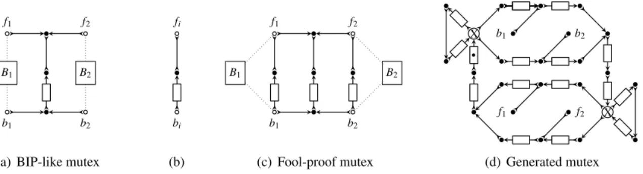
(d) Generated mutex Figure 2: Fool-proof (c) mutual exclusion protocol in Reo, composed from a BIP-like (a) mutual exclu-sion connector and an altenator connector (b), and the generated Reo circuit (d) from Example 5.
Example 3. Figure 2(a) shows a Reo connector that achieves mutual exclusion of componentsB1 and
B2, exactly as the BIP system shown in Figure 1 does. This connector consists of a composition of channels and nodes in Table 1. The Reo connector atomically accepts data from eitherb1orb2and puts it into theFIFO1 channel, a buffer of size one. A fullFIFO1 channel means thatB1 or B2 holds the lock. If one of the components writes to f1or f2, theSyncDrainchannel flushes the buffer, and the lock is released, returning the connector to its initial configuration, whereB1andB2 can again compete for exclusive access by attempting to write tob1orb2.
Note that this connector is not fool-proof. Even ifB1 takes the lock, B2 may release it, and vice versa. Hence, exactly as the BIP architecture in Figure 1, the Reo connector in Figure 2(a) relies on the conformance of the coordinated componentsB1andB2. The expected behaviour ofBi, i=1,2, is that it alternates writes on thebi and fi, and that every write on fi comes after a write onbi. Depending on such assumptions may not be ideal. The connector, shown in Figure 2(b), makes this expected behaviour explicit. By composing two such connectors with the connector in Figure 2(a), we obtain a fool-proof mutual exclusion protocol, as shown in Figure 2(c). Figure 4(c) shows the constraint automaton seman-tics of the connector in Figure 2(c). Unlike the case of the connector in Figure 2(a) or the BIP architecture in Figure 1, non-compliant writes tobi or fi ports of the connector in Figure 2(c) willblockcomponent
Bi, but cannotbreakthe mutual exclusion protocol that this connector implements. 4
Formal semantics of Reo. Reo has a variety of formal semantics [4, 16]. In this paper we use its operationalconstraint automaton(CA) semantics [8].
Definition 7 (Constraint automata [8]). Let N be a set of nodes and D a set of data items. A data constraint is a formula in the language of the grammar
g→ > | ¬g|g∧g| ∃dp(g)|dp=v, withp∈N ,v∈D,
where variabledp represents the data assigned to (i.e., exchanged through) port p. Let|=denote the obvious satisfaction relation between data constraints and data assignmentsδ :N→D, withN⊆N,
and writeDC(N,D)for the set of all data constraints. A constraint automaton (over data domainD) is a tupleA = (Q,N ,→,q0)where Qis a set of states, N is a finite set of nodes, → ⊆Q×2N ×
DC(N ,D)×Qis a transition relation, andq0∈Qis the initial state.
Sync LossySync SyncDrain FIFO1 Node
A B A B A A0 A B
•
B A
B0 A0
q
{A,B},>
q
{A,B},>
{A},>
q
{A,A0},>
q0 q1 {A},>
{B},>
q
{B,A,A0},>
{B0,A,A0},>
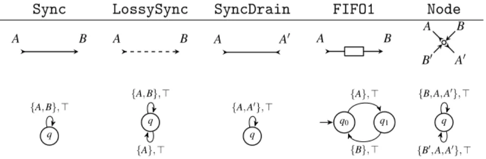
Table 1: Some primitives in the Reo language with CA semantics over a singleton data domainD.
to define any data assignment. For notational convenience, we relax, in this paper, the definition of data constraints and allow the use of set-membership and functions in the data constraints. However, we preserve the intention that a data constraint describes a set of data assignments.
Table 1 shows the CA semantics for some typical Reo primitives. The CA semantics of every Reo connector can be derived as a composition of the constraint automata of its primitives, using the CA product operation in Definition 8. On the other hand, every constraint automaton (over a finite data domain) translates back into a Reo connector [7]. Because of this correspondence, we may consider Reo and CA as equivalent, and focus on constraint automata only.
If a constraint automatonA has only one state,A is calledstateless. If the data domainD ofA is a singleton, A is called a port automaton[17]. In that case, we omit data constraints, because all satisfiable constraints reduce to>.
Definition 8 (Product of CA [8]). Let Ai = (Qi,Ni,→i,q0,i) be a constraint automaton, for i=1,2. Then the productA1onA2of these automata is the automaton(Q1×Q2,N1∪N2,→,(q0,1,q0,2)), whose transition relation is the smallest relation obtained by the rule:(q1,q2)
N1∪N2,g1∧g2
−−−−−−−→(q01,q02)whenever
1. q1 N1,g1
−−−→1q01,q2 N2,g2
−−−→2q02, andN1∩N2=N2∩N1, or
2. qi Ni,gi
−−→iq0i,Nj=/0,gj=>,q0j=qj, andNi∩Nj=/0 with j∈ {1,2} \ {i}.
It is not hard to see that constraint automata product operator is associative and commutative modulo equivalence of state names and data constraints.
Definition 9(Hiding in CA [8]). LetA = (Q,N ,→,q0)be a constraint automaton, andP={p1, . . . ,pn} a set of nodes. Then hiding nodesPofA yields an automaton∃P(A) = (Q,N \P,→∃,q0), where→∃ is given by{(q,N\P,∃dp1· · · ∃dpn(g),q
0)|(q,N,g,q0)∈ →}.
The hiding operator affects only transition labels, and preserves the structure of the automaton. Hence the hiding operator offers a technique to alter the interface of a component or connector without mod-ifying its behaviour. As hiding of non-shared nodes distributes over the product, hiding of non-shared nodes commutes with constraint automata product.
Example 4(Product and hide). Consider the Reo connectors in Figure 2. Using Definition 8, and the primitive constraint automata from Table 1, we find their CA semantics as shown in Figures 4(a), 4(b), and 4(c), respectively. If we compute the product of the automatonA0in Figure 4(a) with the automata
Ai,i=1,2, in Figure 4(b), then we obtain an automatonA, whose part reachable from the initial state
Reo BIP
PA Arch
LTS f1
bip1
g1 reo1
[8]
[7] [6]
(a) data-agnostic domain
Reo BIP
CA± IM
LTS f2
bip2
g2 reo2
[8]
[7] [11]
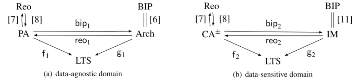
(b) data-sensitive domain Figure 3: Translations and interpretations in data-agnostic and data-sensitive domain.
3
Port automata and BIP architectures
To study the relation between BIP and Reo with respect to synchronization, we start by defining a cor-respondence between them in the data-agnostic domain. This corcor-respondence consists of a pair of map-pings between the sets containing semantic models of BIP and Reo connectors. For the data independent semantic model of Reo connectors we choose port automata: a restriction of constraint automata over a singleton set as data domain. We model BIP connectors by BIP architectures introduced in [6]. In order to compare the behaviour of BIP and Reo connectors we interpret them as labeled transition sys-tems. We define a mappingreo1 that transforms BIP architectures into port automata, and a mapping bip1that transforms port automata into BIP architectures. We then show that these mappings preserve (1) properties closed under bisimulation, and (2) composition structure modulo semantic equivalence.
3.1 Interpretation of BIP and Reo
To compare the behaviour of BIP and Reo connectors, we interpret all connectors as labeled transitions systems with one initial state and an alphabet 2P, for a set of portsP. We write LTS for the class of all such labeled transition systems.
Figure 3(a) shows our translations and interpretations. The objects PA, Arch and LTS are, respec-tively, the classes of port automata, BIP architectures, and labeled transition systems. The mappings bip1,reo1,f1andg1, respectively, translate Reo to BIP, BIP to Reo, Reo to LTS, and BIP to LTS.
We first consider the semantics of connectors. Since BIP connectors differ internally from Reo connectors, we restrict our interpretation to their observable behaviour. This means that we hide the ports of the coordinating components in BIP architectures. For port automata this means that for our comparison, we implicitly assume that all names represent boundary nodes.
The interpretation of a port automaton in LTS is defined by
f1((Q,N,→,q0)) = (Q,2N,→,q0). (1)
Hencef1acts essentially as an identity function, justifying our choice of interpretation. Next, we define the interpretation of BIP architectures using their operational semantics obtained by applying them on dummy components and hiding all internal ports. LetA= (C,P,γ)be a BIP architecture with
coordi-nating componentsC ={C1, . . . ,Cn},n≥0, andCi= (Qi,q0i,Pi,→i). Recall thatPC =
S
iPi is the set of internal ports inA. Define D= ({qD},qD,P,{(qD,N,qD)| /06=N ⊆P\PC})as a dummy compo-nent relative to the BIP architectureA. Using Definition 3, we compute the BIP architecture application
A({D}) = ((∏ni=1Qi)× {qD},(q0,qD),P,→s)ofAto its dummy componentD. Then,
g1(A) = (∏ni=1Qi× {qD},2P\PC,{((q,qD),N\PC,(q0,qD))|(q,qD) N
0 1
{b1} {b2}
{f1}
{f2}
(a) BIP-like mutex
0
1
{bi} {fi}
(b)
0,0,0 1,1,0
0,1,1
{b1}
{b2} {f1}
{f2}
(c) Fool-proof mutex
q
/0
{b1,b12}
{b2,b12}
{f1,f12} {f2,f12}
(d)Aγ12
f ree,q
taken,q
/0
/0
{b1} {b2} {f1}
{f2}
(e)reo1(A12)
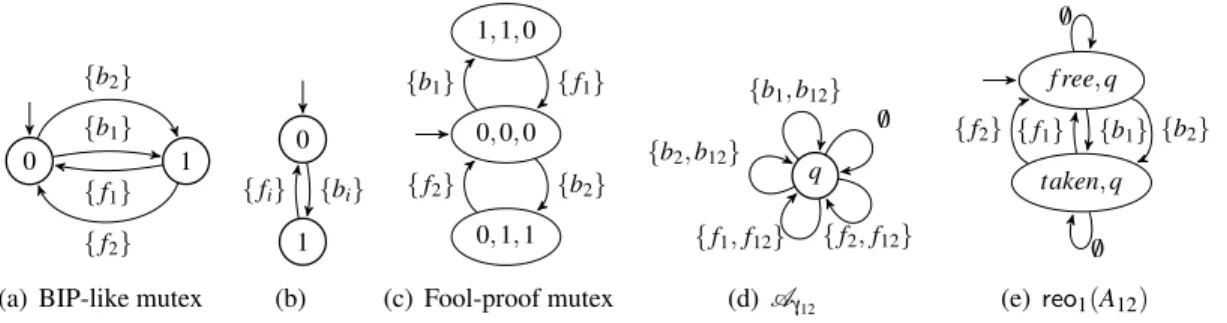
Figure 4: CA representations(a),(b), and (c) of Reo connectors Figures 2(a), 2(b), and 2(c), respec-tively; translation of the interaction model(d)and BIP architecture(e)of Figure 1.
In other words,g1(A)equalsA({D})after hiding all internal portsPC. Note that we based our interpreta-tiong1on the operational semantics of BIP architectures, i.e., BIP architecture application. This justifies the definition of interpretation of architectures.
Because of hiding,g1is not injective. Hence, our interpretation of BIP architectures induces a non-trivial equivalence given by equality of interpretations. In the sequel, we use a slightly stronger version of equivalence based on bisimulation [19].
Definition 10(Bisimulation [19]). IfLi= (Qi,2Pi,→i,q0i)∈LTS,i=1,2, thenL1andL2 arebisimilar (L1∼=L2) iffP1=P2and there existsR⊆Q1×Q2such that(q01,q02)∈R, and(q1,q2)∈Rimplies, for all
N∈2Pi,i,j∈ {1,2}withi6= j, ifq i
N
−→iq0i, then, for someq0j,qj N
−→jq0jand(q01,q02)∈R.
Definition 11(Semantic equivalence). LetA,B∈PA be port automata andA,B∈Arch be BIP archi-tectures. Then,A andB are semantically equivalent(A ∼B) ifff1(A)∼=f1(B), andA andBare
semantically equivalent(A∼B) iffg1(A)∼=g1(B).
With a common semantics for BIP and Reo, we can define the notion of preservation of properties expressible in this common semantics. Recall that a property of labeled transition systems corresponds to the subset of labeled transition systems satisfying that property.
Definition 12. LetP⊆LTS be a property. Then,bip1preserves Pifff1(A)∈P⇔g1(bip1(A))∈Pfor allA ∈PA. Similarly,reo1preserves Piffg1(A)∈P⇔f1(reo1(A))∈Pfor allA∈Arch.
3.2 BIP to Reo
To translate BIP connectors to Reo connectors, we first determine what elements of BIP architectures correspond to Reo connectors. Our interpretations of port automata and BIP architectures show that dangling ports in BIP architectures correspond to boundary port names in port automata. Furthermore, the mutual exclusion of the interactions in an interaction model in a BIP architecture simulates mutually exclusive firing of transitions in port automata. The definition of a coordinating component in a BIP architecture is almost identical to that of a port automaton, yielding an obvious translation.
LetA= (C,P,γ) be a BIP architecture, withC ={C1, . . . ,Cn}. EachCi corresponds trivially to a port automatonCei. LetAγ= ({q},P,→,q)be the stateless port automaton overPwith transition relation →defined by{(q,N,q)|N∈γ}. ThenAγ can be seen as the port automata encoding of the interaction
modelγ. Recall thatPC =S
C∈CPC. The corresponding port automaton ofAis given by
Example 5. We translate the BIP architecture in Example 1 using (3). First, we transformγ12 into a port automatonAγ12, shown in Figure 4(d). Then, we compute the product ofAγ12with the coordinating
componentC12 to obtain the port automaton corresponding to the BIP architectureA12, shown in Fig-ure 4(e). As mentioned in section Section 2.2, we can transform the port automaton in FigFig-ure 4(e) into a Reo connector, using the method described in [7]. This mechanical translation yields the Reo connector in Figure 2(d). Here, the dot in the FIFO1 buffer indicates that its initial state is the full state. The crossed node represents anexclusive router, which atomically takes data from a coincident sink end, and provides it to a single coincident source end. Note that the port automaton semantics of the connector in Figure 2(a) (see Figure 4(a)) is similar to the automaton in Figure 4(e), up to empty transitions. 4
3.3 Reo to BIP
In BIP, interaction is memoryless. This means that a stateful channel in Reo must translate to a coordi-nating component. In fact, we may encode the whole Reo connector as one such component.
LetAi,i=1,2, be two port automata, and let p∈N1∩N2be a shared port ofA1andA2. Suppose that we know how to translate Ai into a BIP architecture Ai. If pis not a dangling port of A1, then, by symmetry, p is not a dangling port ofA2. But now, A1 andA2 are not composable, because there components are not disconnected. Hence, since we want the translation to preserve composition, p
should be a dangling port.
LetA = (Q,N ,→,q0)be a port automaton. We construct a corresponding BIP architecture. Du-plicate all ports inN by definingN0={n0|n∈N}for allN⊆N. We do not use a portn0, forn∈N, for composition. Their exact name is therefore not important, but merely their relation to its dangling brothern. Trivially,A = (Q,q0,N 0,→c), with→c={(q,N0,q0)|(q,N,q0)∈ →}, is a BIP component (cf., Definition 1). Essentially,A andA are the same labeled transition system. Now we define:
bip1(A) = ({A},N ∪N0,{N∪N0|N⊆N}). (4)
Thus,bip1uses the port automaton as the coordinating component of the generated BIP architecture.
Example 6. LetA be the port automaton in Figure 4(b) over the name setN ={bi,fi}. We determine bip1(A). Obtain A by adding adding a prime to each port inA. The interaction model ofbip1(A) consist of{N∪N0|N⊆N }=/0,{bi,b0i},{fi,fi0},{bi,b0i,fi,fi0} .Hence,bip1(A)is given by th BIP architecture({A},{bi,fi,b0i,fi0},
/0,{bi,b0i},{fi,fi0},{bi,b0i,fi,fi0} ).
3.4 Preservation of properties
To confirm that translationsreo1 andbip1 preserve properties, we first investigate whether Figure 3(a) commutes, i.e.,f1(reo1(A)) =g1(A)andg1(bip1(A)) =f1(A), forA∈Arch andA ∈PA.
First, note that the equationsf1(reo1(A)) =g1(A) andg1(bip1(A)) =f1(A)cannot hold, because their state spaces differ. For example,g1alters the state space by adding the state of a dummy component, andreo1adds the state of the port automaton encoding of the interaction model. Therefore we view these equations modulo bisimulation of labeled transition systems from Definition 10.
in stateq0i andCj is in stateq0j. However, BIP semantics does not allow independent progress of state-changing empty-labeled transitions, which means that this single transition exists only whenq0i=qi and
q0j =qj. Indeed, the first rule of Definition 3 allows eitherCi orCj to change state, and the second rule implies q0i =qi and q0j =qj for N = /0. Because of this, we need to exclude BIP architectures where two coordinating components can make a state-changing empty-labeled transition. Moreover, as we consider composition of BIP architectures in Section 3.5, we exclude BIP architectures containing a single coordinating component that can make a state-changing empty-labeled transition, and restrict Arch to Arch0 ={A∈Arch| ∀Ci∈C : qi
/0 −
→i q0i⇒q0i=qi}. Finally, consider the equationg1(bip1(A))∼= f1(A), for some port automaton A. Note that the interaction model of bip1(A) contains the empty set. Hence, the second rule in Definition 3 yields empty-labeled self-transitions ing1(bip1(A)). Since f1 acts like the identity, we conclude that A should have empty-labeled self-transitions, i.e., q0=q implies(q,/0,q0)∈ →. On the other hand, suppose that(q,/0,q0)∈ →. Then the coordinating component ofbip1(A) should not contain a state-changing empty-labeled transition, henceq0=q. Therefore, we
restrict PA to PA0={A ∈PA|q→−/0 q0⇔q0=q}.
Theorem 1. For allA ∈PA0and A∈Arch0 we haveg1(bip1(A))∼=f1(A)andf1(reo1(A))∼=g1(A).
Proof. Using Definition 3, Definition 8, A∈Arch0, A ∈PA0, and the fact that (qD,/0,qD)∈ →/ D, it follows that (1)∼given by(q,qD)∼qfor allq∈Qis a bisimulation betweeng1(bip1(A))andf1(A), whereQis the state space ofA, and (2) ≈given by(q,qI)≈(q,qD)for allq= (qi)i∈I ∈∏i∈IQi, is a bisimulation, whereQi,i∈I, are the state spaces of the coordinating components ofA. See [14] for a detailed proof.
Corollary 1. bip1 andreo1 preserve all properties closed under bisimulation, i.e., for all P⊆LTS,
A ∈PA0and A∈Arch0we havef1(A)∈P⇔g1(bip1(A))∈P andg1(A)∈P⇔f1(reo1(A))∈P. Example 7. Consider the following safety property ϕ satisfied by the Reo connector in Figure 2(c): “ifb1 fires, thenb2fires only after f1 fires”. Clearly, the automatonA0, obtained from Figure 4(c) by adding empty self-transitions, satisfies this property as well. Using Corollary 1, we conclude that the BIP architecturebip1(A) =bip1(A0)satisfiesϕ. More generally, Corollary 1 allows model checking of
BIP architectures with Reo model checkers. 4
3.5 Compatibility with composition
BIP architectures and port automata have their own notions of composition. This raises the question of whether our translations preserve composition structures. We show that, under specific conditions, our translations preserve composition modulo semantic equivalence. Recall the port automaton representa-tion of the interacrepresenta-tion model (Secrepresenta-tion 3.2).
Lemma 1. Let Ai= (Ci,Pi,γi)∈Arch, i=1,2, with PC1∩PC2 = /0and /0∈γ1∩γ2. Then, we have that
Aγ12∼Aγ1 onAγ2, whereγ12be the interaction model of A1⊕A2.
Proof. Follows easily from Definition 8 and Definition 4. See [14] for a detailed proof.
Suppose thatreo1(A1⊕A2)∼reo1(A1)onreo1(A2), for any two BIP architectures A1,A2∈Arch0. Definition 8 impliesNreo1(A1⊕A2)=Nreo1(A1)onreo1(A2)=Nreo1(A1)∪Nreo1(A2). In other words, the name set
of port automaton reo1(A1⊕A2) is the union of the name set of the port automata reo1(Ai), i=1,2. Hence,Nreo1(Ai)⊆Nreo1(A1⊕A2), fori=1,2. This means that the dangling ports ofreo1(A1⊕A2)contain
Note that this is only a mild assumption. Indeed, if p∈PC1∩P2is a dangling port ofP2, connected directly to a component inA1. Then, we first add a (dangling) portx toA1 and synchronize p with p0 by considering the BIP interaction modelγ10 ={N∪ {x} |p∈N∈γ1} ∪ {N|p∈/ N∈γ}. Finally, we renameptoxinA2. The resulting architectures satisfy the assumption.
Theorem 2. reo1(A1⊕A2)∼reo1(A1)onreo1(A2)for all Ai= (Ci,Pi,γi)∈Arch0, with PC1∩P2=PC2∩ P1=/0and/0∈γ1∩γ2.
Proof. LetC1∪C2={C1, . . . ,Cn, . . . ,Cm}, withCi ∈C1 iffi≤n. By definition, we have reo1(A1⊕
A2) =∃PC1∪C2(Cf1on· · ·Cfn onCgn+1on· · ·CfmonAγ12). Next, we use the bisimulation of port automata
(i.e., constraint automata with data contraint>) as defined in [8]. Composition (on) of port automata is commutative and associative up to bisimulation [8]. Using Lemma 1, it follows thatreo1(A1⊕A2)∼= ∃PC1∃PC2(Cf1on· · ·CfnonAγ1 noCgn+1on· · ·CfmonAγ2). Indeed, sincef1is like the identity, it follows that
semantic equivalence∼coincides with bisimulation'of port automata as defined in [8]. Now, we use our assumption thatPC1∩P2=PC2∩P1=/0, and the fact thatCf1, . . . ,Cfn, andAγ1 do not use ports from PC2. Then,reo1(A1⊕A2)=∼∃PC1(Cf1on· · ·CfnonAγ1)on∃PC2(Cgn+1on· · ·CfmonAγ2)). We conclude that
reo1(A1⊕A2)∼=reo1(A1)onreo1(A2). Since, f1 is like the identity, it is not hard to see that f1 takes bisimilar port automata to bisimilar labeled transition systems. Therefore,reo1 is a homomorphism up to semantic equivalence, i.e.,reo1(A1⊕A2)∼reo1(A1)onreo1(A2).
Theorem 3. bip1(A1onA2)∼bip1(A1)⊕bip1(A2)for allAi∈PA0.
Proof. Note that, sincef1is like the identity, semantic equivalence∼coincides with bisimulation'of port automata [8]. As'is a congruence with respect to the compositiononof port automata, we conclude
that∼is a congruence too (i.e.,f1(Ai)∼=f1(Ai0), fori=1,2, impliesf1(A1onA2)∼=f1(A10onA20)). Let Ai ∈PA0, i=1,2, be two port automata. From Theorem 2, we conclude that f1(reo1(A1⊕
A2))∼=f1(reo1(A1)onreo1(A2)), for any A1,A2∈Arch0. SubstituteAi =bip1(Ai), fori=1,2. Then, f1(reo1(bip1(A1)⊕bip1(A2)))∼=f1(reo1(bip1(A1))onreo1(bip1(A2))). Thus, f1(reo1(bip1(Ai)))∼= g1(bip1(Ai))∼=f1(Ai), for i=1,2, by Theorem 1. Hence, using that ∼ is a congruence, we ob-tain g1(bip1(A1)⊕bip1(A2))∼=f1(A1 onA2). Therefore, g1(bip1(A1)⊕bip1(A2))∼=g1(bip1(A1on A2)).
Example 8. For any two portsxandy, letA{x,y}be the port automaton of a synchronous channel (cf., Ta-ble 1), and letC{x,y}be its corresponding BIP component. Suppose we need to translateA{a,b}onA{b,c} to a BIP architecture. Then we first computebip1(A{a,b}) = ({C{a0,b0}},{a,a0,b,b0},γ{a,b}), withγ{a,b}= {/0,{a,a0},{b,b0},{a,a0,b,b0}}. Next, we computebip1(A{b,c}) = ({C{b00,c00}},{b,b00,c,c00},γ{b,c}), with
γ{b,c}={/0,{b,b00},{c,c00},{b,b00,c,c00}}. Note that we need to use a double prime now, because oth-erwiseb0 would be a shared port ofC{a0,b0} andC{b00,c00}. Using Theorem 3, we find thatbip1(A{a,b}on
A{b,c}=bip1(A{a,b})⊕bip1(A{b,c}) = ({C{a0,b0},C{b00,c00}},{a,a0,b,b0,b00,c,c00},γ{a,b,c}), where γ{a,b,c} is the composition ofγ{a,b}andγ{b,c}.
4
Stateless CA’s and interaction models
In Section 3 we established a correspondence between port automata and BIP architectures. Here, we offer translations between data-aware connector models in BIP and Reo.
First we determine the semantic model of the connectors. For BIP connectors we use BIP interac-tion models, i.e., sets of interacinterac-tion expressionsα, with a single top port that is not a bottom port, and
whose guard and up functions are independent of local variables (Definition 5). We assume that every top port occurs only in one interaction expression per BIP interaction model. We denote the class of BIP interaction models by IM. For the semantics of Reo connectors we take a pair consisting of a constraint automaton together with a partition of its node set into source nodesNsrc, mixed nodesNmix, and sink nodesNsnk. We call such pairsconstraint automata with polarity. Due to the absence of coordinating components in the data sensitive model for BIP, we restrict ourselves here to stateless constraint au-tomata, since BIP interaction expressions are stateless [6, 11]. We write CA±for the class of all stateless constraint automata with polarity, with Nsrc =P∗={p∗| p∈P} and Nsnk=P∗ ={p∗| p∈P} for some set of portsP. This assumption is necessary to enable simulation of bidirectional ports in BIP. The reason we explicitly distinguish node types in this semantics is to give direction to dataflow, similar to BIP connectors. Usually such node type distinctions are implicit, but for preciseness we encode them as a partition within the semantics of Reo connectors.
As in Section 3, we interpret all connectors as labeled transition systems. Then we define translations between Reo connectors (CA±) and BIP connectors (IM), and show that they preserve properties.
4.1 Interpretation of BIP and Reo
An important difference between BIP and Reo involves how they handle data. BIP uses bidirectional ports, while Reo treats input and output ports separately. Since the common semantics should support both approaches, we duplicate every bidirectional port of BIP to obtain two unidirectional ports, compat-ible with Reo. The sense of every reference to a bidirectional port in a BIP interaction expression maps that bidirectional port to its intended corresponding unidirectional port.
Let LTS be the class of all labeled transition systems over an alphabet(D+1)2P, where Dis a set of data items; 1={0} containsvoid ornull, modeling the absence of data; and 2P is theduplicated (unidirectional) port setof a set of (bidirectional) portsP, that is, 2P={p∗,p∗|p∈P}. If data appears atp∗(i.e.,δ(p∗)6=0 forδ∈(D+1)2P), then we interpret this as input to the connector. If data appears
atp∗, then we interpret this at output from the connector.
Consider Figure 3(b). Classes CA±and IM consist of constraint automata with polarity and interac-tion models. Morphismsbip2andreo2are translations of those classes andf2andg2are interpretations in a common LTS semantics. We do not intend to redefine the semantics of constraint automata with polar-ity and of interaction models in this section. Hence, we interpret them using their definitions from [8,11]. We begin by defining the interpretation of stateless constraint automata with polarity. Given a state-less constraint automaton with polarityA, we first determine the smallest set of bidirectional portsP
such thatNsrcused ⊆P∗ and Nsnkused ⊆P∗, where N used
src andNsnkused are all source and sink nodes that occur on a transition of A. Then, we take 2P as the port names of f2(A). Finally, we obtain the transitions of f2(A) by replacing every transition labeled with N,g inA with a set of transitions la-beled with δ ∈∆(N,g), where ∆(N,g) contains all data assignments δ : 2P→D+1 that satisfy the
data constraintN,g. We formalize this as follows. LetA = ({q},Nsrc,Nmix,Nsnk,→,q)be a stateless constraint automaton with polarity over a data domainD. DefineNsrcused =
S
{N∩Nsrc|q N,g
Nused snk =
S
{N∩Nsnk|q N,g
−−→q}. LetPbe the smallest set, withNsrcused⊆P∗andNsnkused⊆P∗. Define
f2(A) = ({q},(D+1)2P,{(q,δ,q)|q N,g
−−→q,δ∈∆(N,g)}), (5)
where ∆(N,g) ={δ : 2P→D+1|δ(2P\N) ={0},δ |=g}. Note that ports in Nsrc\Nsrcused and
Nsnk\Nsnkusedare important only for composition, which we do not consider in this paper.
Next, we interpret interaction modelsΓ by a single-state labeled transition system with labels de-scribing all possible dataflows allowed by the guard, and up and down functions of some interaction expression inΓ. Before we provide a formal definition, we first introduce some notation. For every BIP
interaction expressionα, we writePα for its bottom ports,gαfor its guard,upαwandupαL for the restric-tion of the up funcrestric-tion to its top port and its local variables, respectively, anddnα
bot for the restriction of the down function to its bottom ports. For every BIP interaction modelΓ, we writePΓ=
S
α∈ΓPα, and
DΓ= S
p∈PΓDp, whereDp is the data type of port p. For every data assignmentδ : 2PΓ →DΓ+1 we
defineδup(p) =δ(p∗)andδdn(p) =δ(p∗), for allp∈Pα. Then, we define
g2(Γ) = ({q},(DΓ+1)2
PΓ,{(q,δ,q)|α∈Γ,δ∈∆(α)⊆(D Γ+1)2
PΓ}), (6)
where∆(α) ={δ |δ(2PΓ\2Pα) ={0},gα(δup) =tt,δdn=dnαbot(upαw(δup),upαL(δup))}. Note that we use the value ofupα
w(δup)as a local variable, since we consider only non-hierarchical interaction models. In [11], Bliudze et al. encode BIP interaction models inTop/Bottom components, i.e., an automaton over interaction expressions together with local variables. Furthermore, they define a semantics for T/B components, which indirectly defines an interpretation of interaction models. Equation (6) imitates this interpretation without using Top/Bottom components explicitly.
Now that we defined the interpretation of our objects in LTS, we explore how these translations preserve properties that are expressible in LTS, as we did for their counterparts in Section 3.1.
4.2 Reo to BIP
Since BIP interaction models are stateless, we cannot translate an arbitrary constraint automaton (i.e., Reo connector) into BIP. Interaction models in BIP preclude keeping track of the state of a Reo connector. Hence, the translation of the interaction model of a BIP architecture into a port automaton in Section 3.2 inspires us for our translationbip2.
LetA be a stateless constraint automaton over a data domainD. Since we care only about external behaviour, we first hide all mixed nodes. Then, we transform every transition inA with labelN,ginto a simple BIP connector withN as its bottom ports, together with a guard, an up and a down function that mimic the data constraintg. We define the corresponding setbip2(A)of simple BIP connectors by the set of all transformed transitions fromA.
We first define the transformation of transitions into interaction expressions. For every labelN,gin automatonA, we define the simple BIP connector
α(N,g) = ({wN,g} ←PN).[gsrc(Xsrc) :Ysnk:=solve(g,Xsrc)//Xsnk:=Ysnk],
wherePN is the smallest set satisfyingN∩Nbnd⊆2PN,gsrc is any quantifier free formula equivalent to ∃N\Nsrc:g, the variablesYsnk={yp|p∈N∩Nsnk}are some fresh local variables, and Xsrc={xp|
deterministic. However, comparing the solve function to the random function in Figure 4 in [11], we see that this generality is justified. Now, we definebip2as follows:
bip2(A) ={α(N,g)|(q,N,g,q)∈ →}, (7)
4.3 BIP to Reo
The correspondence between BIP interaction expressions and automata transitions from Section 4.2, provides the main idea for the translation of interaction models into stateless constraint automata. IfΓis a set of simple BIP connectors, we assign to everyα ∈Γa transitionτα labeled withN(α),g(α), and
subsequently construct the stateless constraint automaton consisting of all suchταtransitions.
Letα be a simple BIP interaction expression. Recall our relaxation on the data constraint language in Section 2, and our notations regardingαin Section 4.1. Then, defineN(α)⊆2Pα={p∗,p∗|p∈Pα}
where p∗∈N(α)iffα assignes data to pin the upward data transfer, and p∗∈N(α)iffα assigns data
topin the downward data transfer. Furthermore, letD∗= (dp∗)p∈P,D ∗= (d
p∗)p∈P, and define
g(α) =Vp∈Pdp∗,dp
∗∈Dp∧gα(D∗)∧D∗=dnbotα (upαw(D∗),upαL(D∗)),
Note thatg(α)is independent of the top portw, as we consider only non-hierarchical connectors.
LetΓbe a set of simple BIP connectors. Recall thatPΓ= S
αPα andDΓ=
S
p∈PΓDp. Then, define
the constraint automatonreo2(Γ)overDΓby
reo2(Γ) = ({q},(PΓ)
∗
,/0,(PΓ)∗,{(q,N(α),g(α),q)|α∈Γ},q). (8)
Example 10. Consider the interaction expressionαmaxfrom Example 2, with the data domains restricted to D={0, . . . ,232−1}. We translate the interaction model Γ={αmax} using (8), i.e., we compute
A =reo2(Γ). Trivially,A is stateless. Its set of input ports equals(PΓ)∗={a∗,b∗}, and its set of output
ports equals (PΓ)∗={a∗,b∗}. It has a unique transitions (q,N,g,q), with synchronization contraint N={a∗,b∗,a∗,b∗}and guardg ≡ Wx,y,z∈D:z=max(x,y)(da∗=x∧db∗=y∧da
∗ =z∧db∗ =z). 4
4.4 Preservation of properties
To show the faithfulness of translationsbip2 andreo2, we show that interpretationsf2andg2commute with the translationsbip2andreo2in Figure 3(b).
Theorem 4. For allA ∈CA±and allΓ∈IMwe haveg2(bip2(A)) =f2(A)andf2(reo2(Γ)) =g2(Γ).
Proof. (Sketch). LetΓ∈IM andA ∈CA±. Then,∆(α(N,g)) =∆(N,g), and∆(N(α),g(α)) =∆(α),
for allα ∈Γ, and all transition labelsN,ginA. From this and the definitions off2andg2, we see that
g2(bip2(A))) =f2(A), andf2(reo2(Γ)) =g2(Γ), respectively.
Corollary 2. The translationsbip2 andreo2 preserve all properties expressible inLTS, i.e.,f2(A)∈
P⇔g2(bip2(A))∈P andg2(Γ)∈P⇔f2(reo2(Γ))∈P for all P⊆LTS,A ∈CA±andΓ∈IM. Example 11. Consider the following safety propertyϕfor the interaction expressionαmaxfrom Exam-ple 2: “the value retrieved from portaequals zero”. Clearly, this safety property does not hold, whenever
aorboffers a non-zero integer. Note thatϕdepends solely on the interpretation of the interaction model Γ={αmax}in LTS, and henceϕis expressible in LTS. Using Corollary 2 we conclude thatϕis false also forAmax=reo2({αmax}). Thus, we know any executable code generated from the constraint automaton
Amax does not satisfy ϕ. More generally, Corollary 2 allows us to use the Reo compiler to generate
5
Conclusions and Future Work
BIP and Reo find common ground in their stimulation of exogenous system design. This means that they force the explicit modeling of coordination constraints. A clear and formal separation between coordination (connectors) and computation (components) allows the software architect to analyze the interaction of the components using automated tools. The exogenous approach of BIP and Reo contrasts with the endogenous approach supported in process algebra and other languages where coordination is woven into the code of the components. For example, process algebra does not supply constructs to enforce the separation of concerns necessary in exogenous coordination [20].
Multiparty synchronization constitutes a fundamental coordination concept in BIP (represented by interactions in a BIP interaction model) and Reo (represented by synchronization constraints in constraint automata). Our translations show that these representations of multiparty synchronization coincide.
The BIP framework concretelydefineswhat separates computation (BIP behaviour) and coordination (BIP interaction), while Reo merelyseparates computation (Reo components) and coordination (Reo connector) structurally. Indeed, Reo does not force a fixed universal definition for computation and coordination in all applications. Without giving a fixed definition of separation criterion, Reo’s structural separation of computation from coordination (i.e., component versus connector) simply means that, while this separation is always important, the distinction between the two is in the eye of the beholder: in different applications, different, or even the same people, may find it convenient to draw the line that separates computation and coordination at different places to suit their needs. For example, the stateful behavior of aFIFOwith capacity of 1 strictly places what this entity does in the behaviour layer of BIP, as a (computation) component. In Reo, such stateful components can, of course, be regarded and used as computation as well. However, when deemed appropriate, one can use the same component (i.e., a
FIFO1channel) in the construction of a Reo connector as well, e.g., to express the stateful, turn-taking interaction between two components, as in Figure 2.
Our data-agnostic translations allow compositional translation, because their operators distribute over composition modulo semantic equivalence. On the other hand, our data-sensitive translation scheme does not support incremental translation. It seems intuitive to translate synchronous Reo channels into BIP interaction expressions. However, the directionality inherent in the dataflows of BIP interaction expres-sions implies that they can compose only hierarchically, whereas therelationalspecification of dataflow constraints in Reo (which manifests itself as data constraints in constraint automata transition labels) al-lows more expressive composition of datafal-lows as relational composition of constraints. This difference restricts the set of the Reo connectors that this scheme can incrementally translate into BIP, as well as the granularity of the sub-connectors that it can translate in one increment: the data constraints on the bound-ary nodes of every such sub-connector must be locally resolvable into a directional dataflow expression at the level of the sub-connector, in isolation. In practice, synchronous cycles in a Reo connector must translate as a whole, which scuttles the computational benefit of translating incrementally.
In contrast with the BIP architecture model, the data-sensitive model for BIP does not include coordi-nating components within the connector [6, 11]. Nevertheless, it seems possible to use the formalization in [11] to extend BIP architectures of [6] with data. However, extending the current composition operator ⊕to compose data-sensitive BIP architectures does not seem trivial, and we do not know what properties such an extended composition operator can preserve.
archi-tectures that may also share internal ports.
References
[1] (2015):BIP toolset. Available athttp://www-verimag.imag.fr/BIP-Tools,93.html.
[2] (2015):Reo toolset. Available athttp://reo.project.cwi.nl/reo/wiki/Tools.
[3] Farhad Arbab (2004): Reo: a channel-based coordination model for component composition. Math. Struc-tures Comput. Sci.14(3), pp. 329–366, doi:10.1017/S0960129504004153.
[4] Farhad Arbab (2011):Puff, The Magic Protocol. In:Talcott Festschrift,Lecture Notes in Comput. Sci.7000, Springer, pp. 169–206, doi:10.1007/978-3-642-24933-4 9.
[5] Farhad Arbab, Roberto Bruni, Dave Clarke, Ivan Lanese & Ugo Montanari (2009): Tiles for Reo. In: Proc. of WADT,Lecture Notes in Comput. Sci.5486, Springer Berlin Heidelberg, pp. 37–55, doi:10.1007/978-3-642-03429-9 4.
[6] Paul Attie, Eduard Baranov, Simon Bliudze, Mohamad Jaber & Joseph Sifakis (2014):A General Framework
for Architecture Composability8702, pp. 128–143. doi:10.1007/978-3-319-10431-7 10.
[7] Christel Baier, Joachim Klein & Sascha Kl¨uppelholz (2014):Synthesis of Reo Connectors for Strategies and
Controllers.Fundam. Inform.130(1), pp. 1–20, doi:10.3233/FI-2014-980.
[8] Christel Baier, Marjan Sirjani, Farhad Arbab & Jan Rutten (2006): Modeling component connectors in Reo
by constraint automata.Sci. Comput. Programming61(2), pp. 75–113, doi:10.1016/j.scico.2005.10.008.
[9] Ananda Basu, Marius Bozga & Joseph Sifakis (2006): Modeling Heterogeneous Real-time Components in BIP. In:Proc. of SEFM, ACM, pp. 3–12, doi:10.1109/SEFM.2006.27.
[10] Simon Bliudze & Joseph Sifakis (2007):The algebra of connectors: structuring interaction in BIP. In:Proc. of EMSOFT, ACM SigBED, ACM, Salzburg, Austria, pp. 11–20, doi:10.1145/1289927.1289935.
[11] Simon Bliudze, Joseph Sifakis, Marius Bozga & Mohamad Jaber (2014):Architecture Internalisation in BIP. In:Proc. of CBSE, ACM, pp. 169–178, doi:10.1145/2602458.2602477.
[12] Roberto Bruni, Hern´an Melgratti & Ugo Montanari (2011): Connector Algebras, Petri Nets, and BIP. In: Proc. of PSI,LNCS7162, Springer, pp. 19–38, doi:10.1007/978-3-642-29709-0 2.
[13] M. Y. Chkouri, A. Robert, M. Bozga & J. Sifakis (2009): Translating AADL into BIP - Application to the Verification of Real-Time Systems. In:Proc. of MODELS,LNCS5421, Springer, pp. 5–19, doi:10.1007/978-3-642-01648-6 2.
[14] K. Dokter, S.-S. T.Q. Jongmans, F. Arbab & S. Bliudze (2015): Relating BIP and Reo. Technical Report FM-1505, CWI. Available athttp://persistent-identifier.org/?identifier=urn:nbn:nl:ui: 18-23505.
[15] David Garlan (2014): Software Architecture: A Travelogue. In: Proc. of FOSE, ACM, pp. 29–39, doi:10.1145/2593882.2593886.
[16] Sung-Shik T. Q. Jongmans & Farhad Arbab (2012):Overview of Thirty Semantic Formalisms for Reo. Sci. Ann. Comp. Sci.22(1), pp. 201–251, doi:10.7561/SACS.2012.1.201.
[17] C. Koehler & D. Clarke (2009): Decomposing port automata. In: Proc. of SAC, ACM, pp. 1369–1373, doi:10.1145/1529282.1529587.
[18] C. Krause (2009):Integrated Structure and Semantics for Reo Connectors and Petri Nets. In:Proc. of ICE, pp. 57–69, doi:10.4204/EPTCS.12.4.
[19] R. Milner (1989):Communication and Concurrency. Prentice-Hall, Inc.
[20] G. A. Papadopoulos & F. Arbab (2001): Configuration And Dynamic Reconfiguration Of Components
Using The Coordination Paradigm. Future Generation Computer Systems 17(8), pp. 1023 – 1038,
[21] Jos´e Proenc¸a & Dave Clarke (2008):Coordination Models Orc and Reo Compared. Electron. Notes Theor. Comput. Sci.194(4), pp. 57–76, doi:10.1016/j.entcs.2008.03.099.
[22] Carolyn Talcott, Marjan Sirjani & Shangping Ren (2011):Comparing three coordination models: Reo, ARC,