Hakkenberg_unc_0153D_16812.pdf

(1)

MAPPING PLANT DIVERSITY AND COMPOSITION ACROSS NORTH CAROLINA PIEDMONT FOREST LANDSCAPES USING LIDAR-HYPERSPECTRAL REMOTE

SENSING

Christopher R. Hakkenberg

A dissertation submitted to the faculty of the University of North Carolina at Chapel Hill in partial fulfillment of the requirements for the degree of Doctor of Philosophy in Ecology in the

Curriculum for the Environment and Ecology.

Chapel Hill 2017

(2)

(3)

ABSTRACT

Christopher R. Hakkenberg: Mapping plant diversity and composition across North Carolina Piedmont forest landscapes using LiDAR-hyperspectral remote sensing

(Under the direction of Conghe Song)

(4)

(5)

(6)

ACKOWLEDGEMENTS

I am humbled to have been able to surround myself with so many fine people these past few years. No doubt, this dissertation project would not have been possible without the support of my advisor, Conghe Song, and a dedicated dissertation committee straddling the realms of Biology and Geography. I’m constantly reminded not just of the quantity of their combined knowledge, but of the quality of their guidance and mentorship. They gave me great independence to explore, to fail, to question my assumptions, and grapple with the implications of my conclusions. I am truly indebted to them – both for their intellectual contributions to the field which established the theoretical foundation from which this work could commence and, selfishly, for their commitment to me, and the goals of this project. Indeed, there is a degree of solemnity in this academic tradition, not just in passing the torch of knowledge, but in imparting the skills with which to wield it.

My classmates and colleagues, with whom I broke bread and corralled countless dogs, were another vibrant source of inspiration. These include Matt Dannenberg, Clare Fieseler, Bianca Lopez, Chris Payne, Dennis Tarasi, Sam Tessel, Sierra Woodruff, and Qi Zhang. Others, informal mentors and collaborators like Jim Clark, Josh Gray, Reuben Valbuena, Alan Weakley, Jack Weiss, and Kai Zhu selflessly offered their time and expertise. And while responsibility for the errors in this document should be placed squarely at my feet, where there is success, it is shared.

(7)

(8)

TABLE OF CONTENTS

TABLE OF CONTENTS ... viii

LIST OF TABLES ... xi

LIST OF FIGURES ... xii

1. INTRODUCTION ... 1

2. FOREST STRUCTURE PREDICTS TREE SPECIES DIVERSITY IN THE NORTH CAROLINA PIEDMONT ... 9

2.1. Introduction ... 9

2.2. Methods ... 11

2.2.1. Study Area ... 11

2.2.2. Forest Inventory Data ... 12

2.2.3. Indices of Taxonomic Diversity ... 14

2.2.4. Indices of Forest Structure ... 15

2.2.5. Data Analysis ... 18

2.3 Results ... 19

2.3.1. Forest Structural Attributes as Predictors of Tree Species Diversity ... 19

2.3.2. Models of Tree Plant Diversity based on Forest Structure ... 22

2.4. Discussion ... 23

2.4.1. Forest Structural Attributes and the Structure-Diversity Relationship ... 23

2.4.2. Predictive Models of Diversity based on Forest Structure ... 26

2.4.3. Structure and Diversity by Stand Origin and Forest Type ... 28

(9)

3. MODELING MULTI-SCALE PLANT SPECIES RICHNESS IN A PIEDMONT NORTH CAROLINA LANDSCAPE USING LIDAR-HYPERSPECTRAL

REMOTE-SENSING ... 31

3.2. Methods ... 34

3.2.1 Study site ... 34

3.2.2. Derived remotely-sensed predictors ... 36

3.3. Results ... 41

3.3.1. Predicting plant species richness across spatial scales ... 41

3.3.2. Remotely-sensed predictors of species diversity ... 47

3.4. Discussion ... 51

3.4.1. Mapping vascular plant species richness at different spatial scales ... 51

3.4.2. Spatial scale constrains remotely-sensed predictors of plant species richness ... 52

3.5. Conclusion ... 60

4. MODELING PLANT COMMUNITY-CONTINUA IN A PIEDMONT FOREST LANDSCAPE WITH LIDAR-HYPERSPECTRAL REMOTE SENSING ... 62

4.2. Methods ... 65

4.2.1. Study site ... 65

4.2.2. Field data ... 66

4.2.3. Remotely-sensed data ... 67

4.3. Results ... 77

4.3.1. Community characterization ... 77

(10)

4.3.3. Remotely-sensed predictors of forest composition ... 84

4.4. Discussion ... 85

4.4.1. From mapping canopy individuals to modeling total stand composition ... 85

4.4.2. Community–continua in compositional and geographical space ... 86

4.4.3. Compositional resolution of community-units ... 87

4.4.4. Gradient mapping of compositional continua ... 91

4.4.5. Remotely-sensed environmental correlates of vascular plant composition ... 92

4.5. Conclusion ... 94

5. CONCLUSIONS ... 96

Appendix 1: FIA North Carolina Piedmont tree species list ... 102

Appendix 2: SVR empirical tuning hyperparameters ... 105

Appendix 3. Relationships among structural variables ... 106

Appendix 4. Spatially nested plot design ... 107

Appendix 5. Duke Blackwood field plot taxa list ... 108

Appendix 6. Remotely-sensed predictors in PCA space ... 112

Appendix 7. Species richness - random forest feature selection ... 113

Appendix 8. Spearman correlation matrix for remotely-sensed variables versus species richness across spatial scales. ... 115

Appendix 9. NMDS Step-down plots ... 116

Appendix 10. NMDS random forest feature selection. ... 117

Appendix 11. NMDS map post-processing. ... 118

Appendix 12. Spearman correlation matrix among all remotely-sensed predictors ... 120

(11)

LIST OF TABLES

Table 2.1. Indices of taxonomic diversity ... 14

Table 2.2. Indices of forest structure ... 15

Table 3.1. Remotely-sensed predictor variables ... 36

Table 3.2. Species richness summary statistics ... 41

Table 3.3. Final species richness predictive models – parameters and results ... 42

Table 4.1. Remotely-sensed predictor variables. ... 72

Table 4.3. Two-class confusion matrix. ... 81

Table 4.4. Seven-class confusion matrix ... 81

(12)

LIST OF FIGURES

Figure 2.1. Piedmont NC study area and FIA plots. ... 11

Figure 2.2. Histogram of FIA plots by stand age and forest type. ... 12

Figure 2.3. Distribution of selected response and predictor variables among all plots and subset by forest type and regeneration method.. ... 18

Figure 2.4. Scatterplots of species richness versus selected predictor variables ... 21

Figure 2.5. Correlation matrix of forest structure versus tree species diversity ... 21

Figure 2.6. Cross-validated adjusted R2 of SVR models ... 22

Figure. 2.7. Importance values based on the R2 statistic of a loess smoother comparing singular predictors to an intercept-only null model. ... 23

Figure 3.1. Duke Forest Blackwood study area extent. ... 35

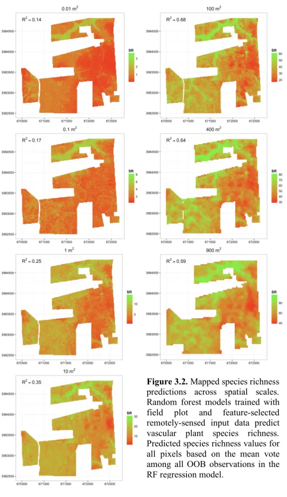
Figure 3.2. Mapped species richness predictions across spatial scales ... 44

Figure 3.3. Mapped species richness predictive uncertainty across spatial scales. ... 45

Figure 3.4. Combined diversity-uncertainty maps across spatial scales. ... 46

Figure 3.5. Spearman correlation matrix for selected remotely-sensed variables versus species richness values across spatial scales ... 47

Figure 3.6. Plant richness ~ LiDAR topography slope parameter posteriors across scales. ... 48

Figure 3.7. Plant richness ~ LiDAR structure slope parameter posteriors across scales ... 48

Figure 3.8. Plant richness ~ hyperspectral slope parameter posteriors across scales ... 50

Figure 4.1. Duke Forest Blackwood study area extent. ... 65

Figure 4.2. Mapped species richness predictions across spatial scales ... 70

Figure 4.3. Field plots classified into two and seven community-unit clusters in NMDS space ... 79

Figure 4.4. Predictive map of vascular plant composition in Duke Forest Blackwood ... 80

(13)

Figure 4.6. NMDS 1-3 environmental biplots ... 84

Figure 4.7. Spearman correlation matrix NMDS 1-3 ~ RS variables ... 85

(14)

CHAPTER 1

INTRODUCTION

The pace of species loss in the Anthropocene has far surpassed background extinction rates, and is only forecasted to accelerate in the near future (Davis & Shaw 2001; Hooper et al. 2012). Perhaps nowhere is this pernicious trend more evident than in the world’s forests. Forests cover approximately 30% of the global land surface, yet account for almost half of terrestrial carbon, and three quarters of terrestrial biodiversity (Kindermann et al. 2008; FAO 2010). But in recent decades, global forests have been profoundly modified, degraded, and destroyed due to the synergistic anthropogenic forces of habitat change, climate change, overexploitation, invasive alien species, and pollution (MEA 2005; Rudel et al. 2005). When these interacting stressors overwhelm ecosystem resilience to environmental and climatic variability, forest ecosystems are at increased risk of harm, including ecological regime shifts and hyperdynamism in ecosystem process rates (Laurance 2002; Walther et al. 2002). Studies have demonstrated the central role of plant diversity for maintaining stability in ecosystem functioning in forest landscapes effected by anthropogenic degradation (Hooper et al. 2002; Folke et al. 2004; Civitello et al. 2015). In fact, a fundamental extrinsic value of biodiversity lies in its potential to provide functionally redundant system components (e.g. species) to regulate ecosystem processes and buffer against anthropogenically-induced environmental change (Elmqvist et al. 2003).

(15)

habitat and serving as nutritional resources for specialist and generalist consumers throughout the trophic chain (Gaston 1992; Myers et al. 2000; Raxworthy et al. 2003; Zak et al. 2003). The central role of plants in constraining forest ecosystem functioning as well as taxonomic, phylogenetic, functional, and biochemical diversity has driven global efforts to model aggregate, emergent properties of forest communities like diversity, species composition, canopy structure, and fucntional traits for applications ranging from landscape-scale ecosystem management, conservation, and habitat modeling, to regional and global modeling of biodiversity and ecosystem function (Gillespie et al. 2008; Abelleira Martinez et al. 2016; Jetz et al. 2016).

(16)

niche conservatism underlying these models is flawed and biotic components completely ignored, niche modeling based purely on coarse abiotic layers may prove inadequate or even misleading.

One effective method to return biological realism to niche modeling is through the incorporation of remotely-sensed data to simultaneously identify underlying environmental gradients constraining the fundamental niche, and directly observe the presence of specific entities occupying their realized niche (Guisan & Zimmermann 2000; Cord et al. 2013). Though remotely-sensed data may be limited in accuracy and precision due to technological and logistical limitations in data acquisition, processing, and analysis, it nonetheless excels for providing a consistent, repeatable, and synoptic - or “wall-to-wall” - census of biophysical factors within the scene extent. In fact, in many cases remotely-sensed data may surpass field-based studies for describing large-scale forest patterns susceptible to spatially-structured environmental filters otherwise concealed amid the complexity of local-scale forest dynamics (Asner et al. 2015).

(17)

(Ustin & Gamon 2010; Ollinger 2011). However, in structurally-complex, continuous-cover forests, optical imagery fails to provide robust data beyond (or below) the upper canopy, and thus offers little to no information on the composition and structural properties of individuals obscured from the sensor’s view. To correct for this lacuna and model the entirety of a stand’s structural elements, from the canopy surface to the shadowed understory, LiDAR has found increasing prominence as a compliment to optical imagery in the remote sensing of vegetation.

(18)

(MacArthur & MacArthur 1961; Moen & Gutiérrez 1997), insects (Recher et al. 1996), and mammals (Sullivan et al. 2001).

Another potential shortcoming with niche modeling, and with SDMs in particular, worth reviewing is the inherent incongruity in the characteristic scales of field plot data (based on sampling size, design, and intensity), remotely-sensed data (such as, spatial resolution and geolocational precision), and that of target biota (e.g. size, density, and coverage extent). This mismatch in scale need not necessarily be problematic. For example, in monospecific forest communities, or in open woodlands where individual tree crowns are spatially distinct and discrete, remotely-sensed pixels may represent a single endmember; that is, pixels may consist entirely of a single plant of sufficient size or cover.However, when scene elements are smaller than the pixel resolution, or when target biota are diverse, intertwined, or otherwise obscured from view, the task of reconciling the disparate scales of data and model may become problematic. Spectral mixing and spatial mismatch between data sources is especially pervasive in structurally and taxonomically heterogeneous forests.

(19)

stacked SDMs (multiple, single-species models), tend to underestimate biotic processes like competition that contribute to observed compositional variance in plot data, and thereby grossly inflate species richness values (Guisan & Rahbek 2011; Clark et al. 2014). Provided predictive models adequately represent the full spectrum of compositional and structural variance observed in field plots, a stand-scale approach enables researchers to model communities holistically, thereby circumventing the problem of failing to predict obscured, and thus undetected, individuals like understory herbs (Ohmann et al. 2011).

Broadly speaking, this study was motivated by the desire to bridge scales of analysis of ecological phenomena from the plot to the landscape, with the ultimate goal to contribute to the better integration of the fields of community ecology, landscape ecology, and remote sensing. Analyses are intended to uncover phenomenological patterns and underlying drivers of forest community properties to map turnover in vegetation composition and diversity across forest landscapes of the North Carolina Piedmont. Spatially nested field sampling, together with burgeoning technologies of LiDAR-hyperspectral remote sensing and emerging statistical techniques like nonparametric predictive community modeling, allow for forest community mapping at scales far finer than that of the nominal resolution of the remotely-sensed data, and at extents far larger than what field sampling would expediently support. Efforts to predict and infer the scale-dependent relationships among remotely-sensed parameters and forest community properties will only grow in the years to come as ecologists anticipate annual NEON data products and the deployment of a fleet of new LiDAR and hyperspectral satellites for use in applications ranging from local-scale land management to global-scale ecosystem modeling.

(20)

North Carolina Piedmont. If so, which structural attributes are most strongly correlated with diversity, and how effective are they when used in concert within a generalized predictive model? To accomplish this goal, I analyze Spearman correlations between 15 measures of forest structure and five indices of tree species diversity based on a set of 972 geographically-distributed Forest Inventory and Analysis (FIA) plots located within North Carolina Piedmont forests (Gray et al. 2012). Next, I combine all predictors in a nonparametric support vector regression (SVR) model to predict tree species diversity in the North Carolina Piedmont based on structure alone, without accounting for other known predictors of diversity, such as environment, soil conditions, and site history. Beyond the theoretical implications of unraveling the underlying relationship between structure (as a surrogate for successional stage) and tree species diversity, this study is designed and implemented to determine the empirical basis for successfully utilizing forest structure from LiDAR remote sensing in predictive models of tree species diversity over large geographic regions.

(21)

addition to spatially-explicit uncertainty maps and accuracy assessment of nonparametric models, hierarchical parametric models are used to infer the relationship between remotely-sensed data and drivers of diversity. This study provides insights into multi-scale landscape turnover of plant diversity, species-area relationships, and remotely-sensible correlates of plant richness.

(22)

CHAPTER 2

FOREST STRUCTURE PREDICTS TREE SPECIES DIVERSITY IN THE NORTH CAROLINA PIEDMONT*

2.1. Introduction

Concerns over global environmental change and biodiversity loss have driven efforts to model the spatial distribution of taxonomic diversity (Ackerly et al. 2010; Hooper et al. 2012). Despite significant progress in recent decades in the modeling of large-scale patterns in biodiversity, direct mapping is still greatly limited by technological and cost constraints (Gaston 2000; Rodrigues & Brooks 2007; Asner & Martin 2009). To improve the estimation of the spatial distribution of diversity over large continuous areas, scalable proxy variables that link ground measurements with remotely-sensed data must be identified and assessed (Kreft & Jetz 2007; Kane et al. 2010; He et al. 2015). Candidate variables should be remotely sensible, ecologically relevant, common in current vegetation inventory databases, as well as temporally dynamic and scalable to larger landscapes (Turner et al. 2003; Anderson & Ferree 2010). This study investigates the utility of employing one such suite of candidate variables, namely those based on forest structure, to predict tree species diversity over large areas of temperate forest.

Forest structure reflects abiotic conditions and site history, including competition and stochastic disturbance events, at multiple spatial scales that affect the three-dimensional distribution of biomass in a forest stand. Several potential mechanisms underlie the relationship _________________________

* This chapter previously appeared as an article in The Journal of Vegetation Science. The original citation is as

follows: Hakkenberg, C.R., Song, C., Peet, R.K., & White, P.S. 2016. Forest structure as a predictor of tree species

(23)

between forest structure and tree species diversity, though no single explanation is diagnostic in assigning causality. On one hand, higher species counts increase the expectation of greater functional diversity in species’ traits. On the other hand, structural complexity begets fine-scale environmental heterogeneity conducive to the partitioning of niche space and the creation of new habitat for a greater diversity of species (Franklin 1988; Palmer & Maurer 1997). These explanations are by no means exhaustive, and without experimental manipulation, teasing apart the causal mechanisms driving these relationships remains problematic.

Observational studies on the effect of stand structure on plant diversity have primarily focused on understory herbaceous species (see Cook 2015 for a review), and to a lesser extent, on tree species diversity. Chiarucci and Bonini (2005), for example, found plot-scale species richness to be significantly related to tree stem density (R2=0.35; p<0.01) and total basal area (R2=0.05; p<0.01), though non-structural, regional predictors like elevation had the highest predictive power (R2 = 0.64). Bacaro et al. (2008) were able to use a host of local and regional predictors to explain 83% of the total variation in woody plant species richness in Tuscan forests, though forest structure accounted for only 1% of non-shared variation in woody richness. Other studies, mainly based on small sample sizes, have tended to find an insignificant or weak correlation between forest structure and woody diversity (Aiba & Kitayama 1999; Neumann & Starlinger 2001). In light of these inconsistent findings and the emergence of remote-sensing technologies like LiDAR as tools for forest biodiversity mapping based on structural surrogates (Rodrigues & Brooks 2007; Wolf et al. 2012; Camathias et al. 2013), further work is needed to evaluate the empirical basis of forest structure as a generalizable predictor of tree species diversity.

(24)

whether forest structure is significantly correlated with tree species diversity in the temperate forests of this region. We then examine which structural attributes are most strongly correlated with tree species diversity, and how effective they are when used in concert in a generalized predictive model. To address these questions, we first focus on characterizing the relationship between individual structural attributes and indices of species diversity. Next, we assess the ability of a generalized machine learning algorithm trained solely with structural variables to predict tree species diversity. Finally, we evaluate cross-validated model performance using the entire NC Piedmont plot database as well as subsets differentiated by stand origin and forest type.

2.2. Methods

2.2.1. Study Area

The study area is located in the central portion of the EPA level 3 “Piedmont” ecoregion and bounded by the state borders of North Carolina (Fig. 2.1) (Griffith et al. 2002). The heavily-forested Piedmont ecoregion, stretching from Northern Virginia to central Alabama, separates the mountainous Appalachians to the northwest from the flat Coastal Plain to the southeast. Once largely dominated by agriculture and grazing lands

! ! ! ! ! ! ! ! ! ! ! ! ! ! ! ! ! ! ! ! ! ! ! ! ! ! ! ! ! ! ! ! ! ! ! ! ! ! ! ! ! ! ! ! ! ! ! ! ! ! ! ! ! ! ! ! ! ! !! ! ! ! ! ! ! ! ! !! ! ! ! ! ! ! ! ! ! !! ! ! ! ! ! ! ! ! ! ! ! ! ! ! ! ! ! ! ! ! ! ! ! ! ! ! ! ! ! ! ! ! ! ! ! ! ! ! ! ! ! ! ! ! ! ! ! ! ! ! ! ! ! ! ! ! ! ! ! ! ! ! ! ! ! ! ! ! ! !! ! ! !! ! ! ! ! ! ! ! ! ! ! ! ! ! !! ! ! ! !! !!! ! ! ! ! ! ! ! ! ! !! ! ! ! ! ! ! !! ! ! ! ! ! ! ! ! ! ! ! ! ! ! ! ! ! ! ! ! ! ! ! !! ! ! ! ! ! ! ! ! ! ! ! ! ! ! ! ! ! !! ! ! !! ! ! ! !! ! ! ! ! !!! ! ! ! ! ! ! ! !! ! ! ! ! ! !! ! ! ! ! ! ! ! ! ! ! ! !! ! ! ! ! ! ! !! ! ! ! ! ! ! ! ! ! ! ! ! ! ! ! ! ! ! ! ! ! ! ! ! ! ! ! ! ! ! ! ! ! ! ! !! ! ! ! ! ! ! ! ! ! ! ! !! ! ! ! ! ! ! ! ! ! ! !! ! !! ! ! ! ! ! ! ! ! ! ! ! !! ! ! ! ! ! ! ! ! ! !! ! ! ! ! ! ! ! ! ! ! ! ! ! ! ! ! ! !! ! ! ! ! ! ! ! ! ! ! ! ! ! ! ! ! ! ! ! ! ! !!! ! ! ! ! ! ! ! ! ! ! ! ! !! ! ! ! ! ! ! ! ! ! ! ! ! ! ! ! ! ! ! ! ! ! ! ! !! ! !! ! ! ! ! ! ! ! ! ! ! ! ! ! ! ! ! ! ! ! ! ! ! ! ! ! ! ! ! ! ! ! ! !! ! ! ! ! ! ! ! ! ! ! ! ! ! ! ! ! ! ! ! ! ! ! !! !! !! ! ! ! ! ! ! ! ! ! ! ! ! ! ! ! ! ! ! ! ! ! ! ! !! ! ! ! ! ! ! ! ! ! ! ! ! ! ! ! ! ! ! ! ! !! ! ! ! ! ! ! ! ! ! ! ! ! ! ! !! ! ! !! ! ! ! ! ! ! ! ! ! ! ! ! ! !! ! ! ! ! !! !! ! ! ! ! ! ! ! ! ! ! ! ! ! ! ! ! ! ! ! ! ! ! ! ! ! ! ! ! ! ! ! ! ! ! ! ! ! ! ! ! ! ! ! ! ! ! ! ! ! ! !! ! ! ! ! ! ! ! ! ! ! ! ! ! ! ! ! ! ! ! !! ! ! ! ! ! ! ! ! ! ! ! ! ! ! ! ! ! !! ! ! ! ! ! ! ! ! ! ! ! !! ! ! ! ! ! ! ! ! ! ! ! ! ! !! ! ! ! ! ! ! ! !! ! ! ! ! ! ! ! ! ! ! ! ! ! ! ! ! ! ! ! ! ! ! ! ! ! ! ! ! ! ! ! ! ! !! ! ! ! ! ! ! ! ! !! !!! ! ! ! ! ! ! ! ! ! ! ! ! ! ! ! ! ! ! ! ! ! ! ! ! !! ! ! ! ! ! ! ! ! ! ! ! ! ! ! ! ! ! ! ! ! ! ! ! ! ! ! !! ! ! ! ! ! ! ! ! ! ! !! ! ! ! ! ! ! ! ! ! ! ! ! ! ! ! ! ! ! ! ! ! ! ! ! ! ! ! ! ! ! ! ! ! !! ! ! ! ! ! ! ! ! ! ! ! ! ! ! ! ! ! ! ! ! ! ! ! ! ! ! !! ! ! !! ! ! ! ! ! ! ! ! ! ! ! ! ! ! ! ! ! ! ! ! ! ! ! ! ! ! ! ! ! ! ! ! ! ! ! ! ! ! ! ! ! ! ! !! ! ! ! ! !! !! ! ! ! ! ! ! ! !! ! ! ! ! ! ! ! ! ! ! ! ! ! ! !!! ! ! ! ! ! ! ! ! !! ! ! ! ! !! ! ! ! ! ! ! ! ! ! ! ! ! ! ! ! ! ! ! ! ! ! ! ! ! ! ! !! ! ! ! ! ! ! ! ! ! ! ! ! ! ! ! ! ! ! ! ! ! ! ! ! ! ! ! ! ! ! ! ! ! ! !! ! ! ! ! ! ! ! ! ! ! ! ! ! ! ! ! ! ! ! ! ! ! ! ! ! ! ! ! ! ! !! ! ! ! ! ! ! ! ! ! ! ! ! ! ! ! ! ! ! ! ! ! ! ! ! ! ! ! ! ! ! ! ! ! ! ! ! ! ! ! ! !! ! ! ! ! ! ! ! ! ! ! ! ! ! ! ! ! ! ! ! ! ! ! ! ! ! ! ! ! ! ! ! ! ! ! ! ! ! ! ! ! ! ! !! ! ! ! ! ! ! ! ! ! ! ! ! ! ! ! ! ! ! ! ! ! ! ! ! ! ! ! ! ! ! !! ! ! ! ! ! ! ! ! ! ! ! ! ! ! ! ! ! ! ! ! ! ! ! ! ! ! ! ! ! !! ! ! ! ! ! ! ! ! ! ! ! ! ! ! ! ! ! !! ! ! ! ! ! ! ! ! ! ! ! ! ! ! ! ! ! ! ! ! ! ! ! ! ! ! ! !! ! ! ! ! ! ! ! ! ! ! ! ! !! ! ! ! ! ! ! ! ! ! ! ! ! ! ! ! ! ! ! ! ! ! ! ! ! ! ! ! ! ! ! ! ! ! ! ! ! ! ! ! ! ! ! ! ! ! ! !! ! ! ! ! ! !! ! ! ! ! ! ! ! ! ! ! ! ! !!! !! ! ! ! ! ! ! ! ! ! ! ! ! ! ! ! ! ! ! ! ! ! !! ! ! ! ! ! ! ! ! ! ! ! !! ! ! ! ! ! ! ! ! !! ! ! ! ! ! ! ! ! ! ! !! ! ! ! !! ! ! ! ! ! ! ! ! ! ! ! ! ! ! ! ! ! ! ! ! ! ! ! ! ! ! ! ! ! ! ! ! ! ! ! ! ! ! ! ! ! ! ! ! ! ! ! ! ! ! ! ! ! ! ! ! ! ! ! ! ! ! ! ! ! ! ! ! ! ! ! ! ! !! ! ! ! ! ! ! ! ! ! ! ! ! ! ! ! ! ! ! ! ! ! ! ! ! ! ! ! ! ! ! ! ! ! ! ! ! ! ! ! ! ! ! ! ! !! ! ! ! ! !! ! ! ! ! ! ! ! ! ! ! ! ! ! ! ! ! ! ! ! ! ! ! !! ! ! ! ! ! ! ! ! ! ! ! ! ! ! ! ! ! ! ! ! ! ! ! ! ! ! ! ! ! ! ! ! ! ! ! ! ! ! ! ! ! ! ! ! ! ! ! ! ! ! ! ! ! ! ! ! ! ! ! ! ! ! ! ! ! !!! ! ! ! ! ! ! ! ! !! ! ! ! ! ! ! ! ! ! ! ! ! ! ! ! ! ! ! ! ! ! ! ! ! ! ! ! ! ! ! ! ! ! ! ! !! ! ! ! ! ! ! ! ! ! ! ! ! ! ! ! ! ! ! ! ! ! ! ! ! ! ! ! ! ! ! ! ! ! ! ! ! ! ! ! ! ! ! ! ! ! ! ! ! ! ! ! ! ! !! ! ! ! ! !! ! ! ! ! ! ! ! ! ! ! ! ! ! ! ! ! ! ! !! ! ! ! ! ! ! ! ! ! ! ! ! ! ! !! ! ! ! !! ! ! ! ! ! ! ! ! ! ! ! ! ! ! ! ! ! ! ! ! ! ! ! ! ! ! ! ! ! ! ! ! ! ! ! ! ! ! ! ! ! ! ! ! ! ! ! ! ! ! ! ! ! ! ! ! ! ! ! ! ! ! ! ! ! ! ! ! ! ! ! ! ! ! ! ! !! ! !! ! ! ! ! !! ! ! !! ! ! ! ! ! ! ! ! ! ! ! ! ! ! ! ! ! ! ! ! ! ! ! ! ! ! ! ! ! ! ! ! ! ! ! ! ! ! ! ! ! ! ! ! ! !! ! ! ! ! ! ! ! ! ! ! ! ! ! ! ! ! ! ! ! !! ! ! ! ! ! ! ! ! ! ! ! ! !! ! ! ! ! ! ! ! ! ! ! ! ! ! ! ! ! ! ! ! ! ! ! ! ! ! ! ! ! ! ! ! ! ! ! ! ! ! ! ! ! ! ! ! ! ! ! ! ! ! ! ! ! ! ! ! ! ! ! ! ! ! ! ! ! ! ! ! ! ! ! ! ! ! ! ! ! ! ! ! ! ! ! ! ! ! ! ! ! ! ! ! ! ! ! ! ! ! ! ! ! ! ! ! ! ! ! ! ! ! ! ! ! ! ! ! ! ! ! ! ! ! ! ! ! ! ! ! ! ! ! ! ! ! ! ! ! ! ! ! ! ! ! ! ! ! ! ! ! ! ! ! ! ! ! ! ! ! ! ! ! ! ! ! ! ! ! ! ! ! ! ! ! ! ! ! ! ! ! !! ! ! ! ! ! ! ! ! ! ! ! ! ! ! ! ! ! ! ! ! ! ! ! ! ! ! ! ! ! ! ! ! ! ! ! ! ! ! ! ! ! ! ! ! ! ! ! ! ! ! ! ! ! ! ! ! ! ! ! ! ! ! ! ! ! ! ! ! ! ! ! ! ! ! ! ! ! ! ! ! ! ! ! ! ! ! ! ! ! ! ! ! ! ! ! ! ! ! ! ! ! ! ! ! ! ! ! ! ! ! ! ! ! ! ! ! ! ! ! ! ! ! ! ! ! ! ! ! ! ! ! ! ! ! ! ! ! ! ! ! ! ! ! ! ! ! ! ! ! ! ! ! ! ! ! ! ! ! ! ! ! ! ! ! ! ! ! ! ! ! ! ! ! ! ! ! ! ! ! ! ! ! ! ! ! ! ! ! ! ! ! ! ! ! ! ! ! ! ! ! ! ! ! ! ! ! ! ! ! ! ! ! ! ! ! ! ! ! ! ! ! ! ! ! ! ! ! ! ! ! ! ! ! ! ! ! ! ! ! ! ! ! ! ! ! ! ! ! ! ! ! ! ! ! ! ! ! ! ! ! ! ! ! ! ! ! ! ! ! ! ! ! ! ! ! ! ! ! ! ! ! ! ! ! ! ! ! ! ! ! ! ! ! ! ! ! ! ! ! ! ! ! ! ! ! ! ! ! ! ! ! ! ! ! ! ! ! ! ! ! ! ! ! ! ! ! ! ! ! ! ! ! ! ! ! !! ! ! ! ! ! ! ! ! ! ! ! ! ! ! ! ! ! ! ! ! ! ! ! ! ! ! ! ! ! ! ! ! ! ! ! ! ! ! ! ! ! ! ! ! ! ! ! ! ! ! ! ! ! ! !! ! ! ! ! ! ! ! ! ! ! ! ! ! ! ! ! ! ! ! ! ! ! ! ! ! ! ! ! ! ! ! ! ! ! ! ! ! ! ! ! ! ! ! ! ! ! ! ! ! ! ! ! ! ! ! ! ! ! ! ! ! ! ! ! ! ! ! ! ! ! ! ! ! ! ! ! !! ! ! ! ! ! ! ! ! ! ! ! ! ! ! ! ! ! ! ! ! ! ! ! ! ! ! ! ! ! ! ! ! ! ! ! ! ! ! ! ! ! ! ! ! ! ! ! ! ! ! ! !! ! ! ! ! ! ! ! ! ! ! ! ! ! ! ! ! ! ! ! ! ! ! ! ! ! ! ! ! ! ! ! ! ! ! ! ! ! ! ! ! ! ! ! ! ! ! ! ! ! ! ! ! ! ! ! ! ! ! ! ! ! ! ! ! ! ! ! ! ! ! ! ! ! ! ! ! ! ! ! ! ! ! ! ! ! ! ! ! ! ! ! ! ! ! ! ! ! ! ! ! ! ! ! ! ! ! ! ! ! ! ! ! ! ! ! ! ! ! ! ! ! ! ! ! ! ! ! ! ! ! ! ! ! ! ! ! ! ! ! ! ! ! ! ! ! ! ! ! ! ! ! ! ! ! ! ! ! ! ! ! ! ! ! ! ! ! ! ! ! ! ! ! ! ! ! ! ! ! ! ! ! ! ! ! ! ! ! ! ! ! ! ! ! ! ! ! ! ! ! ! ! ! ! ! ! ! ! ! ! ! ! ! ! ! ! ! ! ! ! ! ! ! ! ! ! ! ! ! ! ! ! ! ! ! ! ! ! ! ! ! ! ! ! ! ! ! ! ! ! ! ! ! ! ! ! ! ! ! ! ! ! ! ! ! ! ! ! ! ! ! ! ! ! ! ! ! ! ! ! ! ! ! ! ! ! ! ! ! ! ! ! ! ! ! ! ! ! ! ! ! ! ! ! ! ! ! ! ! ! ! ! ! ! ! ! ! ! ! ! ! ! ! ! ! ! ! ! ! ! ! ! ! ! ! ! ! ! ! ! ! ! ! ! ! ! ! ! ! ! ! ! ! ! ! ! ! ! ! ! ! ! ! ! ! ! ! ! ! ! ! ! ! ! ! ! ! ! ! ! ! ! ! ! ! ! ! ! ! ! ! ! ! ! ! ! ! ! ! ! ! ! ! ! ! ! ! ! ! ! ! ! ! ! ! ! ! ! ! ! ! ! ! ! ! ! ! ! ! ! ! ! ! ! ! ! ! ! ! ! ! ! ! ! ! ! !! ! ! ! ! ! ! ! ! ! ! ! ! !! ! ! ! ! ! ! ! ! ! ! ! ! ! ! ! ! ! ! ! ! ! ! ! ! ! ! ! ! ! ! ! ! ! ! ! ! ! ! ! ! ! ! ! ! ! ! ! ! ! ! ! ! ! ! ! ! ! ! ! ! ! ! ! ! ! ! ! ! ! ! ! ! ! ! ! ! ! ! ! ! ! ! ! ! ! ! ! ! ! ! ! ! ! ! ! ! ! ! ! ! ! ! ! ! ! ! ! ! ! ! ! ! ! ! ! ! ! ! ! ! ! ! ! ! ! ! ! ! ! ! ! ! ! ! ! ! ! ! ! ! ! ! ! ! ! ! ! ! ! ! ! ! ! ! ! ! ! ! ! ! ! ! ! ! ! ! ! ! ! ! ! ! ! ! ! ! ! ! ! ! ! ! ! ! ! ! ! ! ! ! ! ! ! ! ! ! ! ! ! ! ! ! ! ! ! ! ! ! ! ! ! ! ! ! ! ! ! ! ! ! ! ! ! ! ! ! ! ! ! ! ! ! ! ! ! ! ! ! ! ! ! ! ! ! ! ! ! ! ! ! ! ! ! ! ! ! ! ! ! ! ! ! ! ! ! ! ! ! ! !! ! ! ! ! ! ! ! ! ! ! ! ! ! ! ! ! ! ! ! ! ! ! ! ! ! ! ! ! ! ! ! ! ! ! ! ! ! ! ! ! ! ! ! ! ! ! ! ! ! ! ! ! ! ! ! ! ! ! ! ! ! ! ! ! ! ! ! ! ! ! ! ! ! ! ! ! ! ! ! ! ! ! ! ! ! ! ! ! ! ! ! ! ! ! ! ! ! ! ! ! ! ! ! ! ! ! ! ! ! ! ! ! ! ! ! ! ! ! ! ! ! ! ! ! ! ! ! ! ! ! ! ! ! ! ! ! ! ! ! ! ! ! ! ! ! ! ! ! ! ! ! ! ! ! ! ! ! ! ! ! ! ! ! !! ! ! ! ! ! ! ! ! ! ! ! ! ! ! ! ! ! ! ! ! ! ! ! ! ! ! ! ! ! ! ! ! ! ! ! ! ! ! ! ! ! ! ! ! ! ! ! ! ! ! ! ! ! ! ! ! ! ! ! ! ! ! ! ! ! ! ! ! ! ! ! ! ! ! ! ! ! ! ! ! ! ! ! ! ! ! ! ! ! ! ! ! ! ! ! ! ! ! ! ! ! ! ! ! ! ! ! ! ! ! ! ! ! ! ! ! ! ! ! ! ! ! ! ! ! ! ! ! ! ! ! ! ! ! ! ! ! ! ! ! ! ! ! ! ! ! ! ! ! ! ! ! ! ! ! ! ! ! ! ! ! ! ! ! ! ! ! ! ! ! ! ! ! ! ! ! ! ! ! ! ! ! ! ! ! ! ! ! ! ! ! ! ! ! ! ! ! ! ! ! ! ! ! ! ! ! ! ! ! ! ! ! ! ! ! ! ! ! ! ! ! ! ! ! ! ! ! ! ! ! ! ! ! ! ! ! ! ! ! ! ! ! ! ! ! ! ! ! ! ! ! ! ! ! ! ! ! ! ! ! ! ! ! ! ! ! ! ! ! ! ! ! ! ! ! ! ! ! ! ! ! ! ! ! ! ! ! ! ! ! ! ! ! ! ! ! ! ! ! ! ! ! ! ! ! ! ! ! ! ! ! ! ! ! ! ! ! ! ! ! ! ! ! ! ! ! ! ! ! ! ! ! ! ! ! ! ! ! ! ! ! ! ! ! ! ! ! ! ! ! ! ! ! ! ! ! ! ! ! ! ! ! ! ! ! ! ! ! ! ! ! ! ! ! ! ! ! ! ! ! ! ! ! ! ! ! ! ! ! ! ! ! ! ! ! ! ! ! ! ! ! ! ! ! ! ! ! ! ! ! ! ! ! ! ! ! ! ! ! ! ! ! ! ! ! ! ! ! ! ! ! ! ! ! ! ! ! ! ! ! ! ! ! ! ! ! ! ! ! ! ! ! ! ! ! ! ! ! ! ! ! ! ! ! ! ! ! ! ! ! ! ! ! ! ! ! ! ! ! ! ! ! ! ! ! ! ! ! ! ! ! ! ! ! ! ! ! ! ! ! ! ! ! ! ! ! ! ! ! ! ! ! ! ! ! ! ! ! ! ! ! ! ! ! ! ! ! ! ! ! ! ! ! !! ! ! ! ! ! ! ! ! ! ! ! ! ! ! ! ! ! ! ! ! ! ! ! ! ! ! ! ! ! ! ! ! ! ! ! ! ! ! ! ! ! ! ! ! ! ! ! ! ! ! ! ! ! ! ! ! ! ! ! ! ! !! ! ! ! ! ! ! ! ! ! ! ! ! ! ! ! ! ! ! ! ! ! ! ! ! ! ! ! ! ! ! ! ! ! ! ! ! ! ! ! ! ! ! ! ! ! ! ! ! ! ! ! ! ! ! ! ! ! ! ! ! ! ! ! ! ! ! ! ! ! ! ! ! ! ! ! ! ! ! ! ! ! ! ! ! ! ! ! ! ! ! ! ! ! ! ! ! ! ! ! ! ! ! ! ! ! ! ! ! ! ! ! ! ! ! ! ! ! ! ! ! ! ! ! ! ! ! ! ! ! ! ! ! ! ! ! ! ! ! ! ! ! ! ! ! ! ! ! ! ! ! ! ! ! ! !! ! ! ! ! ! ! ! ! ! ! ! ! ! ! ! ! ! ! ! ! ! ! ! ! ! ! ! ! ! ! ! ! ! ! ! ! ! ! ! ! ! ! ! ! ! ! ! ! ! ! ! ! ! ! ! ! ! ! ! ! ! ! ! ! ! ! ! ! ! ! ! ! ! ! ! ! ! ! ! ! ! ! ! !! ! ! ! ! ! ! ! ! ! ! ! ! ! ! ! ! ! ! ! ! ! ! ! ! ! ! ! ! ! ! ! ! ! ! ! ! ! ! ! ! ! ! ! ! ! ! ! ! ! ! ! ! ! ! ! ! ! ! ! ! ! ! ! ! ! ! ! ! ! ! ! ! ! ! ! ! ! ! ! ! ! ! ! ! ! ! ! ! ! ! ! ! ! ! ! ! ! ! ! ! ! ! ! ! ! ! ! ! ! ! ! ! ! ! ! ! ! ! ! ! ! ! ! ! ! ! ! ! ! ! ! ! ! ! ! ! ! ! ! ! ! ! ! ! ! ! ! ! ! ! ! ! ! ! ! ! ! ! ! ! ! ! ! ! ! ! ! ! ! ! ! ! ! ! ! ! ! ! ! ! ! ! ! ! ! ! ! ! ! ! ! ! ! ! ! ! ! ! ! ! ! ! ! ! ! ! ! ! ! ! ! ! ! ! ! ! ! ! ! ! ! ! ! ! ! ! ! ! ! ! ! ! ! ! ! ! ! ! ! ! ! ! ! ! ! ! ! ! ! ! ! ! ! ! ! ! ! ! ! ! ! ! ! ! ! ! ! ! ! ! ! ! ! ! ! ! ! ! ! ! ! ! ! ! ! ! ! ! ! ! ! ! ! ! ! ! ! ! ! ! ! ! ! ! ! ! ! ! ! ! ! ! ! ! ! ! ! ! ! ! ! ! ! ! ! ! ! ! ! ! ! ! ! ! ! ! ! ! ! ! ! ! ! ! ! ! ! ! ! ! ! ! ! ! ! ! ! ! ! ! ! ! ! ! ! ! ! ! ! ! ! ! ! ! ! ! ! ! ! ! ! ! ! ! ! ! ! ! ! ! ! ! ! ! ! ! ! ! ! ! ! ! ! ! ! ! ! ! ! ! ! ! ! ! ! ! ! ! ! ! ! ! ! ! ! ! ! ! ! ! ! ! ! ! ! ! ! ! ! ! ! ! ! ! ! ! ! ! ! ! ! ! ! ! ! ! ! ! ! ! ! ! ! ! ! ! ! ! ! ! ! ! ! ! ! ! ! ! ! ! ! ! ! ! ! ! ! ! ! ! ! ! ! ! ! ! ! ! ! ! ! ! ! ! ! ! ! ! ! ! ! ! ! ! ! ! ! ! ! ! ! ! ! ! ! ! ! ! ! ! ! ! ! ! ! ! ! ! ! ! ! ! ! ! ! ! ! ! ! ! ! ! ! ! ! ! ! ! ! ! ! ! ! ! ! ! ! ! ! ! ! ! ! ! ! ! ! ! ! ! ! ! ! ! ! ! ! ! ! ! ! ! ! ! ! ! ! ! ! ! ! ! ! ! ! ! ! ! ! ! ! ! ! ! ! ! ! ! ! ! ! ! ! ! ! ! ! ! ! ! ! ! ! ! ! ! ! ! ! ! ! ! ! ! ! ! ! ! ! ! ! ! ! ! ! ! ! ! ! ! ! ! ! ! ! ! ! ! ! ! ! ! ! ! ! ! ! ! ! ! ! ! ! ! ! ! ! ! ! ! ! ! ! ! ! ! ! ! ! !! ! ! ! ! ! ! ! ! ! ! ! ! ! ! ! ! ! ! ! ! ! ! ! ! ! ! ! ! ! ! ! ! ! ! ! Piedmont

North Carolina

0 25 50 100 150 200

Kilometers

$

!

FIA Plots

(25)

(including upland hardwood forests), the NC Piedmont has largely reverted to old-field successional pine and hardwood forest (Peet & Christensen 1988).

Plant species richness levels in the NC Piedmont tend to be strongly correlated with soil nutrient content, soil moisture and parent material (Peet & Christensen 1980; Peet & Christensen 1988; Peet et al. 2014). At local scales (100-1000 m2), the highest levels of species richness occur in riparian communities, in moist but well-drained sites (Matthews et al. 2011). Upland forest species richness, on the other hand, is driven primarily by soil chemistry and especially base cations, phosphorus availability, and soil moisture (Peet & Christensen 1980). Despite the large spatial extent of the study area, the narrow range of variability in elevational and latitudinal range limits the influence of climatic factors, thereby allowing us to focus exclusively on the relationship between structure and tree diversity (National Climatic Data Center 2011).

2.2.2. Forest Inventory Data

Vegetation plot data were drawn from the USDA Forest Service’s Forest Inventory and Analysis (FIA) database, the largest and most comprehensive forest inventory and monitoring program in the US, with remeasurement of all plots occurring on a 5-10 year cycle. (Gray et al. 2012). Under the nationally-consistent inventory design, plot locations are geographically-distributed throughout a base grid, with individual plots selected to assign one plot for each 2428 ha

0 20 40 60 80

0 50 100 150

Stand Age

Plot Count

Forest Type

Pine (n=198)

Mixed (n=308)

Broadleaf (n=466)

Figure 2.2. Histogram of FIA plots by stand age

(26)

hexagon across the US (O’Connell et al. 2015). Within each plot, trees (>12.7 cm DBH) were measured on each of four 7.3m radius subplots (O’Connell et al. 2015). Stem counts were converted to a per-unit-area metric using the FIA’s subplot expansion factors, at a spatial scale capable of capturing the range of variability in stand structure (Clebsch & Busing 1989; Busing & White 1993; Bechtold & Patterson 2005). Due to concerns over landowner privacy, as well as plot integrity and vandalism of plot locations on public lands, the precise locations of FIA plots are “fuzzed”, such that plot locational precision is limited to one mile, and “swapped”, where up to 20% of private plot location coordinates are swapped with similar plots within the same county (O’Connell et al. 2015). To ensure that plot locations retain their anonymity while still conforming to the specific spatial extent of our study area, the Forest Service assisted in the provision of the final plot list used in this analysis (USDA 2014, database accessed July, 2015).

(27)

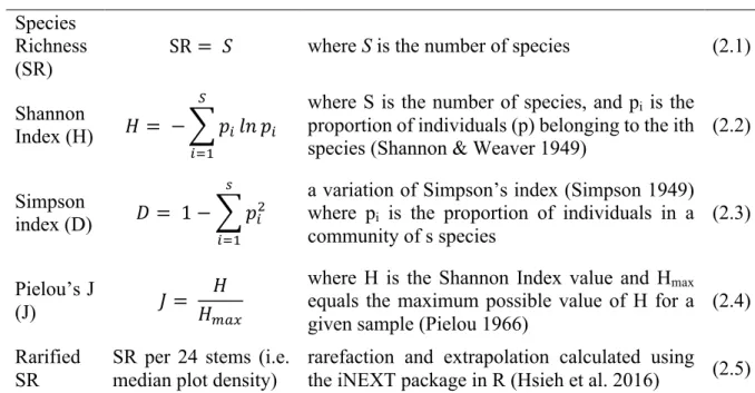
Table 2.1. Indices of taxonomic diversity Species

Richness (SR)

SR = 𝑆 where S is the number of species (2.1)

Shannon

Index (H) 𝐻 = − 𝑝)𝑙𝑛 𝑝) ,

)-.

where S is the number of species, and pi is the proportion of individuals (p) belonging to the ith species (Shannon & Weaver 1949) (2.2) Simpson

index (D) 𝐷 = 1 − 𝑝)1 2

)-.

a variation of Simpson’s index (Simpson 1949) where pi is the proportion of individuals in a community of s species

(2.3)

Pielou’s J

(J) 𝐽 =

𝐻 𝐻₄₅₆

where H is the Shannon Index value and Hmax equals the maximum possible value of H for a given sample (Pielou 1966)

(2.4)

Rarified SR

SR per 24 stems (i.e. median plot density)

rarefaction and extrapolation calculated using the iNEXT package in R (Hsieh et al. 2016) (2.5)

2.2.3. Indices of Taxonomic Diversity

We used five commonly-used and ecologically-interpretable indices of taxonomic diversity, that each emphasize a different aspect of species diversity (Peet 1974; Magurran 1988): species richness (SR), the Shannon’s H and Simpson’s D indices of entropy, Pielou’s J measure of evenness, and rarified species richness (rarified SR) (Table 2.1). Despite the parsimony in tallying species for a given area, species richness fails to account for the distribution of relative abundances, making inference and comparison across communities of varying densities problematic. Therefore the Shannon index (H) - which is more sensitive to rarer species - andthe Simpson index (D= 1-Simpson’s 1949 index; Simpson 1949) - which responds more to abundant species - were included to represent two points in a spectrum of relative sensitivity to species number versus relative evenness (Hill 1973; Peet 1974; Heip et al. 1998). Pielou’s J (J; Pielou 1966) was used to approximate evenness of species presence (Jost 2010).

(28)

the number of expected species (Bunge & Fitzpatrick 1993). Rarefaction enables a comparison of species richness between stands of varying density by re-sampling individuals to simulate species accumulation curves at equivalent stem density (Gotelli & Colwell 2001). Rarified SR values were calculated from a coverage-based sampling curve based on a Monte Carlo re-sampling procedure on all plots (Chao & Jost 2012). Interpolated (rarified) and extrapolated (predicted) richness values were then estimated from this sampling curve based on an expectation of equivalent density corresponding to the median density of all plots (i.e. 24 individual stems or 0.14 stems per m2) (Chao & Jost 2012).

2.2.4. Indices of Forest Structure

Structural indices quantify attributes such as abundance and size variation in the standing biomass in the horizontal plane (e.g. stem density and basal area), as well as the vertical dimension (e.g. canopy heights, foliar profile, and stratification)(Davis & Roberts 2000; Gadow et al. 2012). A host of numerical methods exist for quantifying and indexing stand structure, though no single authoritative set of criteria exists, making direct comparison problematic (Neumann & Starlinger 2001; Staudhammer & LeMay 2001). For this study, we selected three classes of easily-measured structural metrics with precedence in the forest ecology literature (Lexerød & Eid 2006): (1) summary statistics, (2) size heterogeneity, and (3) size distribution statistics (Table 2.2).

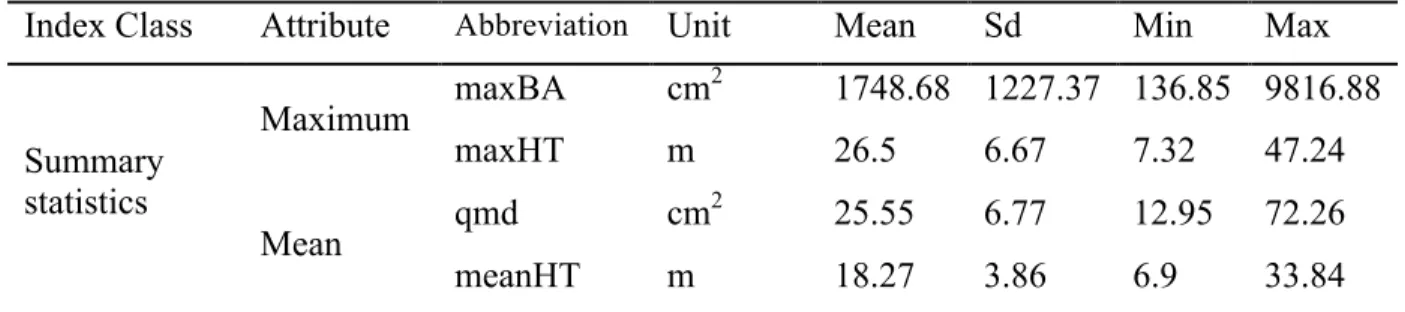
Table 2.2. Indices of forest structure. (“BA” - basal area; “HT” - height; “qmd” - quadratic mean

diameter; “ST” - stems; “-” – unitless)

Index Class Attribute Abbreviation Unit Mean Sd Min Max

Summary statistics

Maximum maxBA cm

2 _{1748.68 1227.37 136.85 9816.88}

maxHT m 26.5 6.67 7.32 47.24

Mean qmd cm

2 _25.55 _6.77 _12.95 _72.26

(29)

Density densityST stems/m2 0.04 0.02 0 0.15

Size

Heterogeneity

Coefficient of

variation (cv)

cvBA - 0.76 0.3 0.02 2.36

cvHT - 0.24 0.09 0.01 0.6

Gini Coefficient (GC)

GCBA - 0.36 0.11 0.01 0.68

GCHT - 0.13 0.05 0 0.28

Size

Distributions Statistics

Skewness skewBA - 1.25 0.86 -0.86 6.35

skewHT - 0.1 0.63 -2.83 3.53

Kurtosis kurtosisBA - 1.45 4.08 -2.75 42.17

kurtosisHT - -0.56 1.7 -2.75 15.4

Weibull (WB)

WBshape - 1.98 3.79 0.65 107.84

WBscale - 589.03 350.98 134.17 5257.4 Basic summary statistics of forest structure include those based on individual stems such as maximum height (maxHT) and maximum basal area (maxBA), and those based on plot-wide statistics such as quadratic mean diameter (qmd), mean height (meanHT) and stem density (densityST). Two measures of structural heterogeneity were selected to indicate dispersion in basal area and height – attributes that have been found to correlate with stand micro-habitats (Acker et al. 1998) and distinguish between successional stages (Spies & Franklin 1991). The coefficient of variation (cv) was chosen owing to its ability to measure relative rather than absolute variation, thereby allowing direct cross-comparison among stands (Weiner & Thomas 1986). The Gini coefficient (GC) is a measure of total inequality in a stand, or the “relative mean difference”, calculated as:

𝐺𝐶 = |𝑥)− 𝑥;|

< ;-. <

)-.

2𝑛1_𝜇 (2.6)

(30)

individuals are equal in size, to a theoretical maximum of one when a stand is dominated by a single individual. Being a statistic of dispersion normalized by the stand mean, GC has the desired property of being independent of density and total BA, thus allowing for comparison between stands (Knox et al. 1989; Valbuena et al. 2012).

The final class of stand structural measures describes higher order moments of the stands’ size distribution, a common indirect method for estimating life table information and stand age structure (Lorimer & Krug 1983). Kurtosis, which estimates the degree of peakedness in the distribution, indicates the extent to which a stand is dominated by modal size classes that loosely track the distribution of age cohorts. Skewness, which measures the degree of asymmetry in the distribution about its mean, has been associated with differences in degree of competition (Knox et al. 1989). We also adopt the Weibull function to describe stand size distribution for its flexible statistical properties and its long history in forestry applications (Weibull 1951; Leak 1964; Bailey & Dell 1973). While there is not a distinct biological basis for this function, it derives its utility from its superior performance in fitting a wide variety stand-size distributions, despite having just two parameters (Rennolls et al. 1985; Jaworski & Podlaski 2011). For a distribution starting at zero, the Weibull probability distribution function is expressed as:

𝑓 𝑥; 𝜆; 𝑘 = 𝑘_𝜆 𝑥_𝜆 CD.

𝑒D 6C F

𝑥 ≥ 0, 0 𝑥 < 0,

(2.7)

(31)

to a negatively-skewed unimodal distribution (k > 3.6). Parameters of the Weibull distribution and their corresponding standard errors were estimated by non-parametric bootstrapping. These three measures of the stand size distribution are attractive because, as continuous variables, they circumvent the issue of information loss and dependency on subjective choice via thresholding and size-class binning (Staudhammer & LeMay 2001; Lexerød & Eid 2006; Valbuena et al. 2012).

Figure 2.3. Distribution of selected response and predictor variables among all plots and subset

by forest type and regeneration method. Violin plots depict distribution of field plots by species richness (SR), maximum height, and basal area heterogeneity (Gini).

2.2.5. Data Analysis

Structural predictors and diversity response variables capture a large spectrum of variation within and between forest types throughout the study area (Fig. 2.3). Data analyses were designed to (1) test the statistical relationship between attributes of forest structure and tree-species diversity based on Spearman’s ρ correlation coefficients, a rank-based measure of association that facilitates application to non-normal data distributions, and (2) evaluate model fit of a series of support vector regression (SVR) predictive models of tree species diversity via 10-fold cross-validation. SVR was chosen over other parametric and machine learning models because of its ability to model nonlinearities in complex datasets, while balancing between high accuracy in response variable prediction and generalizability to unseen data (Vapnik & Vapnik 1998; Schölkopf & Smola 2002).

0.0 0.2 0.4 0.6

All st

ands Pine _Mixed

Broadlea f

Natural Artficial

B asal A rea het erogeneit y (G ini) 4 8 12 16

All st

ands _{Pine Mixed} Broadlea

f

NaturalArtficial

species Richness (S R) 10 20 30 40

All st

f

NaturalArtficial

Forest type subset

Maximum Height 0.0 0.2 0.4 0.6

All st

f

NaturalArtficial

B asal A rea het erogeneit y (G ini) 4 8 12 16

All st

f

NaturalArtficial

species richness (S R) 10 20 30 40

All st

f

NaturalArtficial

Forest type subset

maximum height 0.0 0.2 0.4 0.6

All st

f

NaturalArtficial

(32)

SVR is an extension of support vector machines (SVM), first developed in statistical learning theory as a machine learning method for classification that has since been extended to prediction and regression (Cortes & Vapnik 1995; Cristianini & Shawe-Taylor 2000). SVMs aim to translate a nonlinear problem to a linear one by using kernel functions to fit a model that maps the original low-dimensional input space into a higher dimensional feature space (Vapnik & Vapnik 1998). The global optimum solution is unique and minimizes overfitting by optimally balancing between the accuracy of the model based on cross-validated training and validation data (Schölkopf & Smola 2002).

Support vector regression (SVR) was performed using a Gaussian radial kernel parameter (γ) and two empirically-determined hyperparameters (C and ɛ) derived from training data (Appendix 2). Variable importance for the SVR model was assessed via the R2 statistic of a loess smoother that compares singular predictors to an intercept-only null model (Kuhn 2008). Model fit between observed and predicted values was assessed using 10-fold cross-validation, an out-of-sample model evaluation procedure whereby random subout-of-samples are iteratively withheld from model training and then used as an independent validation of model results. While out-of-sample validations may result in a lower goodness of fit than in-sample tests, they are unbiased and provide a better measure of a model’s predictive accuracy, especially when generalized to independent data (Hastie et al. 2009). All statistical analyses were performed using the software R, v. 3.2.1 (R Core Team 2016), with SVR model training and variable importance calculated using the caret package (Kuhn 2015) and coverage-based rarified species richness performed using the iNEXT package (Hsieh et al. 2016).

2.3 Results

(33)

(34)

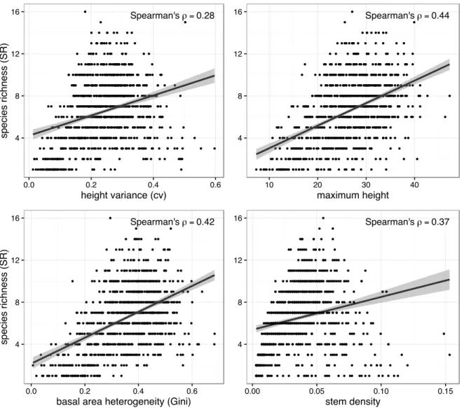
Figure 2.4. Scatterplots of species richness versus selected predictor variables. Linear regression line (black) and 95% confidence intervals (grey).

Figure 2.5. Correlation matrix of forest structure versus tree species diversity. Spearman correlation coefficients. Non-zero values significant at p<0.05.

0 20 40 60 80

0 50 100 150

Stand Age P lot Count Forest Type Pine (n=198) Mixed (n=308) Broadleaf (n=466) Spearman'sρ=0.28

4 8 12 16

0.0 0.2 0.4 0.6

height variance (cv)

species

richness

(S

R)

Spearman'sρ=0.44

4 8 12 16

10 20 30 40

maximum height

Spearman'sρ=0.42

4 8 12 16

0.0 0.2 0.4 0.6

basal area heterogeneity (Gini)

species

richness

(S

R)

Spearman'sρ=0.37

4 8 12 16

0.00 0.05 0.10 0.15

stem density -1 -0.8 -0.6 -0.4 -0.2 0 0.2 0.4 0.6 0.8 1 maxB A

maxHT meanHT qmd densit yST

cvB A

cvHT GCB

A

GCHT skewB A skewHT kurt osisB A kurt osisHT

WBshapeWBscale

(35)

2.3.2. Models of Tree Plant Diversity based on Forest Structure

Support vector regression (SVR) models run on the full dataset (n=972 plots) explained 55% of the variance in predicted SR values, and 60%, 61%, 44% and 59% of variance in predicted values for Shannon’s H, Simpson’s D, rarified SR, and Pielou’s J, respectively (Fig. 2.6). When subset by stand origin (natural and artificially planted/seeded) and forest type (pine, mixed, and broadleaf), predictive accuracy was highest for artificially-regenerated and pine-dominated stands. This trend was especially pronounced for diversity indices most sensitive to relative abundance, like Pielou’s J (R2=0.71 and R2=0.66 for artificially-regenerated and pine stands, respectively). In general, tree species diversity in the broadleaf (0.21 < R2 < 0.52) and mixed categories (0.39 < R2 < 0.56) exhibited the lowest

degree of predicted accuracy. Relative variable importance of structural attributes based on the full SVR model revealed a relationship between individual structural predictors and diversity indices

SR

Shannon's H

Simpson's D

rarified SR

Pielou's J

BroadleafMixed Pine ArtificialNatural Full

0.00 0.25 0.50 0.75 1.00

SVR model cross−validatedR2values

Figure 2.6. Cross-validated adjusted R2 of SVR

(36)

resembling those observed with Spearman correlations, with size dispersion generally exhibiting the largest influence on predictive models, followed by maximum size and Weibull shape (Fig. 2.7).

Figure. 2.7. Importance values based on the R2_{statistic of a loess smoother comparing singular}

predictors to an intercept-only null model. Predictors assessed for the full dataset.

2.4. Discussion

2.4.1. Forest Structural Attributes and the Structure-Diversity Relationship

2.4.1.1. Summary statistics: maximum, mean and density

Spearman correlation coefficients confirm the first hypothesis that measureable components of forest structure are significantly correlated with a range of taxonomic diversity indices, though the strength of this relationship varies greatly among structural attributes. Corroborating results from other studies, we found a significant correlation between diversity and stand maximum values like maxHT and maxBA across all diversity indices (Aiba & Kitayama 1999; Wolf et al. 2012). While stand maximum values partly reflect the growth traits of constituent species whose presence may not necessarily be driving species, they can also be characteristic of underlying site factors that drive productivity and diversity levels, such as site index and time since

SR rarified SR Shannon's H Simpson's D Pielou's J

WBscale kurtosisHT kurtosisBA skewHT skewBA GCHT GCBA cvHT cvBA densityST qmd meanHT maxHT maxBA

0.0 0.2 0.4 0.0 0.2 0.4 0.0 0.2 0.4 0.0 0.2 0.4 0.0 0.2 0.4

(37)

stand-replacing disturbance (Franklin 1988; Peet & Christensen 1988). Stand-wise means such as qmd, meanHT, and WBscale, in contrast, were only weakly significant predictors of tree species diversity, partially reflecting information loss due to averaging across individuals.

Of particular note in assessing these results is the shifting role of stem density across diversity indices. While density may vary with species richness simply by virtue of sampling effect, it may likewise reflect biologically meaningful patterns in successional stage and resource availability that can influence community assembly processes (Weiner & Thomas 1986; Goodburn & Lorimer 1999; Gotelli & Colwell 2001). Results confirmed our expectation that the magnitude of correlation between density and diversity tracks the relative influence of species number versus evenness across the spectrum of diversity indices. Thus, while density had the highest correlation with species richness, it was not significantly correlated with rarified SR, species evenness, Shannon’s H, or Simpson’s D - all measures designed to be independent from this density-dependent sampling effect.

2.4.1.2. Size heterogeneity: cv and Gini

(38)

through succession and its impact on resource levels and competition (Franklin 1988; Palmer & Maurer 1997). More specifically, the development of increasing structural complexity through succession affects patterns of diversity and composition by driving absolute changes in resource levels as well as the spatial variability of the individuals exploiting those resources (Peet 1992; Halpern & Spies 1995).

In keeping with the Piedmont old-field model of succession, disturbance and competition drive temporal dynamics in stand structure, characterized by a progression from structurally simple to more complex, multi-cohort stands (Peet & Christensen 1987). This pattern of increasing structural complexity through time reflects findings from other locations that confirm structural heterogeneity as an effective proxy for stand age and population structure (Lorimer & Krug 1983; Uuttera et al. 1997; Lexerød & Eid 2006). Spatially heterogeneous resource distributions, in turn, drive changes in light penetration and root competition that may increase the probability for recruitment of a variety of species not necessarily present in the stand overstory, including suppressed understory individuals as well as recruits newly dispersed or emergent from the seed bank (Canham et al. 1994; Montgomery & Chazdon 2001). Increased microsite heterogeneity drives niche-space partitioning and other community assembly processes that allow for greater species packing within a given area (Shmida & Wilson 1985).

2.4.1.3. Size distributions: skewness, kurtosis, and Weibull shape

(39)

1983; Knox et al. 1989). Whereas even-aged stands tend toward unimodal Gaussian size-class distributions, uneven-aged stands exhibit a negative monotonic diameter distribution, culminating in the balanced diameter distribution of the highly skewed reverse-J form (Goodburn & Lorimer 1999; Rubin et al. 2006). The reverse-J reflects later successional canopy dynamics, namely when a highly abundant gap-regenerated younger cohort coincides with remaining large-canopy dominants that, despite their scarcity, retain a high proportion of stand basal area (Leak 1964; Bailey & Dell 1973).

Skewness and WBshape (a measure of skewness of the Weibull distribution) were highly correlated with species diversity, with left-skewed distributions characterized by positive skewness and negative Weibull shape values. In either case, the left-skewed distributions of uneven-aged forests tend toward higher tree species diversity levels. These results match findings from other studies in the North Carolina Piedmont reporting species richness to peak in late succession following gap development and understory re-initiation when strands simultaneously possess shade-tolerant, climax species and early-successional colonizers (Peet & Christensen 1988). Kurtosis, on the other hand, appeared to have only limited utility in representing cohort structure, primarily because high kurtosis values can be suggestive both of structurally-simple, single-cohort stands, as well as multi-cohort, later successional stands characterized by the reverse-J basal-area distribution or fat-tailed, unimodal distributions. These confounding patterns are partly responsible for the weak to non-significant correlation between kurtosis values and tree species diversity.

2.4.2. Predictive Models of Diversity based on Forest Structure

(40)

generalizability, we found SVR models trained solely with structural attributes explain more than half of the variance observed in tree species diversity across the full Piedmont dataset. Individual structural attributes were selected for their potential to reflect components of stand structure readily measured on the ground and at larger spatial scales using remote sensing products including LiDAR, Interferometric Synthetic Aperture Radar (InSAR), and optical time series data (Hyde et al. 2006; Bergen et al. 2009; Song et al. 2015). At present, airborne LiDAR scanners are capable of detecting canopy structural elements with <10cm vertical and horizontal precision, and explain 50-95% of the variance in many of the ground-measured structural attributes used in this study, including mean height, maximum height, stem density, and basal area (Næsset 2002; Cook et al. 2013). In this way, the utility of using forest structure as a parameter for landscape-scale predictive mapping of tree species diversity is derived from its ability to indirectly account for variation in diversity levels otherwise caused by latent but difficult to measure factors like soil conditions and site history (Beier & de Albuquerque 2015). These results confirm the empirical relationship between structure and diversity, and thus, the basis for its use as an effective surrogate in modeling species diversity – one that would likely be improved greatly with the inclusion of topographic, environmental, and land cover data.

(41)

Weak correlations found in studies using large national inventories to investigate regional patterns of diversity may reflect a design focusing on maximizing plant diversity prediction through the inclusion of other types of environmental predictors (Chiarucci & Bonini 2005; Bacaro et al. 2008). Depending on the variance partitioning method, covariance between structure and other more significant environmental predictors could obscure the predictive power of structural variables when used alone, a factor noted by Bacaro et al. (2008). Finally, weak correlations found in previous studies could result from inherent limitations of the statistical models used, such that assumptions about linearity, normality, and collinearity in parametric models may constrain their predictive ability and generalizability to independent data (Vapnik & Vapnik 1998; Dormann et al. 2013). Although distribution-free kernel methods like SVR are not immune to multi-collinearity, redundancy in collinear predictors is minimized when the data are translated into a higher-dimensional feature space (Schölkopf & Smola 2002; Toloşi & Lengauer 2011). What the black box SVR model loses in lack of transparency of parameter estimation and standard errors, it more than regains in flexibility and statistical power.

2.4.3. Structure and Diversity by Stand Origin and Forest Type

(42)

single-cohort, monospecific pine plantations (e.g. Pinus taeda), and to a lesser extent mixed-species, multi-cohort stands. Structurally-simple planted stands tend towards monospecificity, whereas multiple-cohort stands with distinct vertical layering between cohorts are more likely to consist of multiple species (Oliver & Larson 1996; Smith et al. 1997). The close relationship between structure and diversity among artificially-regenerated stands reflects the fact that small changes in structure likely coincide with compositional change. Successional stands have been found to show a strong pattern of low diversity during the early self-thinning phase of development, followed by a steady increase with the opening of the canopy (Peet 1992). In the case of an even-aged, monospecific Pinus-dominated overstory, the establishment of a single new understory hardwood in a canopy gap would double species richness – a dramatic change in diversity levels, readily observed in the structural signal. While a broad range of silvicultural practices exist that maintain multi-strata, multi-species stands, natural forests in our dataset tend, by comparison, to a broader range of compositional types and structural forms that tend to be less correlated with structural attributes (Smith et al. 1997).

When subset by forest type and leaf habit, tree species diversity in the pine category was predicted with the highest accuracy. As with artificially-regenerated stands, pine-dominated forests in the Piedmont tend to be early-successional, single-cohort, structurally simple, and near monospecific. Unlike dense-canopy, early-successional pine stands, those undergoing gap formation open themselves to recruitment, thereby increasing their likelihood for higher species richness (Peet 1992). As with natural forests, the broadleaf and mixed forest categories include a wider range of forest types and highlight some of the inherent limitations to modeling species diversity based on structure in more species-rich broadleaf forests.

(43)

(44)

CHAPTER 3

MODELING MULTI-SCALE PLANT SPECIES RICHNESS IN A PIEDMONT NORTH CAROLINA LANDSCAPE USING LIDAR-HYPERSPECTRAL

REMOTE-SENSING

3.1. Introduction

(45)

One promising technology in this pursuit is hyperspectral imaging, or image spectroscopy, which provides highly spectrally-resolved data on the reflectance properties of forest canopies (Ghiyamat & Shafri 2008; Im & Jensen 2008). Hyperspectral imaging exploits the fact that spectral reflectance can be diagnostic of phenotypic traits like foliar morphology and biochemistry (Curran 1989). Even when the mechanistic relationships between spectral reflectance and the contingencies of trait - environment interactions are not fully resolved, correlational relationships between narrowband spectral features (only partially observable using broadband instruments) and foliar chemistry allow for the detection of a host of canopy properties including stand composition and underlying environmental conditions (Ustin & Gamon 2010; Ollinger 2011). While intra-species trait variation and canopy structure can confound consistent spectral retrievals (Castro-Esau et al. 2006; Knyazikhin et al. 2013), to the extent that inter-species variation in foliar biochemistry manifests as heterogeneity in the spectral reflectance signal in a local neighborhood, spectral variance has been observed to correlate with taxonomic diversity (Rocchini et al. 2010; Cavender-Bares et al. 2016).

(46)

canopy height from LiDAR first returns, topo-physiognomy from LiDAR ground returns, biophysical structure from LiDAR all returns, and canopy biochemistry from image spectroscopy (Anderson et al. 2008; Dalponte et al. 2008; Torabzadeh et al. 2014). In fact, combined LiDAR-hyperspectral datasets have been found to more accurately characterize canopy composition and distribution than either used separately (Asner et al. 2008; Feilhauer & Schmidtlein 2009).

Hyperspectral-LiDAR systems are adept in the direct remote detection of species and that of species diversity through the direct detection of structural and biochemical heterogeneity (Rocchini et al. 2010). Moreover, they excel as a data source for the mapping of geophysical gradients from which multi-species niche models, and therefore landscape patterns in biodiversity, can be constrained (Elith & Leathwick 2009; Ohmann et al. 2011). When paired with field plots, remotely-sensed data on canopy reflectance and structure allows for robust prediction of landscape turnover in plant diversity and provides a basis for inference concerning the underlying drivers and merging patterns of diversity at spatial extents far larger than traditional field sampling would allow. Most studies in biodiversity modeling focus on empirical relationships between remotely-sensed data and levels of species diversity (Cayuela et al. 2006; Rocchini et al. 2007; Simonson et al. 2012; Camathias et al. 2013; Higgins et al. 2014). Other studies have employed these empirical relationships in a predictive mapping format (Ohmann & Gregory 2002; Leutner et al. 2012; Wolf et al. 2012; Fricker et al. 2015). With some notable exceptions (e.g. Gould 2000; Schmidtlein & Sassin 2004; Simonson et al. 2012), most remotely-sensed diversity mapping studies have focused on woody canopy species, at a single spatial scale.

(47)

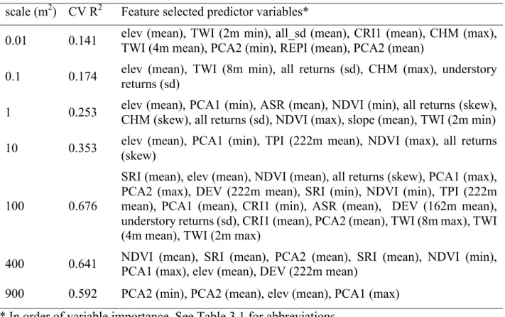
plot data (sampling size, design, and intensity), remotely-sensed data (spatial resolution and geolocational precision), species diversity patterns (species-area relationships), and that of target biota (size, density, and coverage extent) are critical to model output. In light of these concerns, this study seeks to explicitly investigate remotely-sensible drivers of plant diversity across multiple spatial scales to contribute to the operationalization of wall-to-wall landscape management and conservation planning for biodiversity in anticipation of annual NEON data products and the deployment of a fleet of new LiDAR and hyperspectral satellites (Kampe et al. 2010; Cook et al. 2013; Dubayah et al. 2014). Specifically, we employ spatially-nested field plots in conjunction with data from the Goddard LiDAR, hyperspectral, thermal (G-LiHT) airborne sensor to map vascular plant species richness at seven spatial scales in a compositionally- and structurally-complex Piedmont forest landscape in North Carolina (NC), USA. To accomplish this goal, this study focuses on three primary tasks. First, we assess how the predictive power of nonparametric models of plant species richness using feature-selected, remotely-sensed data, changes across seven spatial scales. Second, we employ these models, trained with remotely-sensed data and spatially-nested field plots, to predict plant species richness across the study area. Finally, we determine the remotely-sensible metrics that correlate with plant species richness in the Piedmont study site and how they change with spatial scale.

3.2. Methods

3.2.1 Study site

(48)

1988). The mapped study area focuses solely on natural and semi-natural forests, and thus excludes areas of plantation forest, clear-cut, and built infrastructure (Fig. 3.1). Field plot locations are based on a stratified random design, such that individual plot locations were randomly pre-determined within the constraints of stratified bands along an east-west and a north-south topographic gradient (Fig. 3.1). The ensuing aspect-elevation combinations ensure field plots span the primary physiognomic types in the study area, including upland, riparian, and bottomland forests, which in aggregate

comprise 0.1% of the entire study area. In all field plots, species presence was recorded following Carolina Vegetation Survey protocols for all vascular plant species in 0.01m2, 0.1m2, 1m2, 10m2, 100m2 spatially-nested subplots, and assessed at the 400m2 and 900m2 scales (Peet et al. 1998). In total, 36 900m2 plots were sampled, each with eight subplots at <100m2 scales (288 plots total) and four subplots per plot at 100m2 (144 plots total). Sub-meter geo-locational precision of all plot and subplot vertices was achieved based on triangulation of Ground Control Points (GCPs) measured in the field with tape measures and in a GIS environment using highly-precise, fine

Figure 3.1. Duke Forest Blackwood study area extent.

The study area excludes areas of plantation forest, clear-cuts, and human habitation. Topographic wetness index (TWI) is a proxy for soil moisture (upper right). Canopy height (lower right) is derived from G-LiHT LiDAR. Elevation (lower left) is featured with ASR (annualized solar radiation) for shading and 2ft (0.6m) contours, with squares representing plot location and extent.

0 250 500 1,000 1,500 2,000 Meters

Canopy Height (m) High : 40 Low : 0 TWI wetness

Wet

Dry

Chapel Hill, NC

ASR

(49)

resolution (0.15m) Digital Orthophoto Quadrangle (DOQ) imagery (NC OneMap Geospatial Portal 2016). Botanical nomenclature follows Weakley (2015). The resultant plot data are available on Vegbank (http://vegbank.org; Peet et al. 2012).

3.2.2. Derived remotely-sensed predictors

Aerial remotely-sensed data come from NASA Goddard's LiDAR, Hyperspectral and Thermal (G-LiHT) airborne imager at a 2m (4m2) spatial resolution and 12-bit radiometric resolution (Cook et al. 2013). The G-LiHT airborne imager utilizes commercial, off-the-shelf sensors a Hyperspec imaging spectrometer (Headwall Photonics, Fitchburg, MA, USA) with a 407–1,007 nm spectral range and a ≤5 nm full width half maximum (FWHM) spectral resolution, as well as a VQ-480 (Riegl USA, Orlando, FL, USA) airborne laser scanning (ALS) system, with a mean return density of up to 50 laser pulses/m2 and 10 cm diameter footprint at the nominal operating altitude of 335m (Cook et al. 2013). Remotely-sensed data used in this study was collected on Oct. 25, 2013, during late-season, leaf-on conditions when inter-species phenological differences could aid in taxonomic discrimination. Thermal data was not available for our study area.

(50)

of variance among all bands. While in the latter case, narrow-band indices with established precedence in the literature were employed (Table 3.1).

Table 3.1. Remotely-sensed predictor variables. All remotely-sensed predictors represent

aggregates of 2x2m pixels resampled to a 30x30m (900m2) output resolution.

Category Predictor Abbv. Equation/Source

LiDAR topography (last returns)

Average Solar

Radiance (annual) ASR (ESRI 2016)

Deviation from

mean elevation DEV

𝐷𝐸𝑉 =MNDM

,O ; where z0 is the elevation