COMPUTATIONAL TECHNIQUES TO ADDRESS THE SIGN PROBLEM IN NON-RELATIVISTIC QUANTUM THERMODYNAMICS
Andrew Christopher Loheac
A dissertation submitted to the faculty at the University of North Carolina at Chapel Hill in partial fulfillment of the requirements for the degree of Doctor of Philosophy in the Department of Physics and
Astronomy in the College of Arts and Sciences.
Chapel Hill 2019
© 2019
ABSTRACT
Andrew Christopher Loheac: Computational Techniques to Address the Sign Problem in Non-Relativistic Quantum Thermodynamics
(Under the direction of Joaquín E. Drut)
TABLE OF CONTENTS
LIST OF FIGURES . . . vii
LIST OF TABLES . . . xiii
LIST OF ABBREVIATIONS . . . xiv
LIST OF SYMBOLS . . . xv
1 Introduction . . . 1
1.1 Dissertation overview . . . 2
1.2 Why are non-relativistic systems interesting? . . . 3
1.3 Brief survey of quantum many-body methods . . . 4
1.4 Experimental counterparts . . . 6
2 Foundations of Interacting Quantum Systems. . . 7
2.1 Equations of state for noninteracting quantum gases on the lattice . . . 8
2.2 Auxiliary field representation of the partition function . . . 10
2.2.1 Hubbard-Stratonovich transformation for contact interactions . . . 12
2.3 Difficulty of direct linear algebra and mean field approaches . . . 16
2.4 Finite-temperature determinantal Monte Carlo . . . 19
2.4.1 Hybrid quantum Monte Carlo . . . 21
2.4.2 Computing observables stochastically . . . 24
3 Strongly Interacting Fermi Gases in One Dimension . . . 27
3.1 Equation of state results for the unpolarized system . . . 28
3.1.1 Calculating the second-order virial coefficient on the lattice exactly . . . 29
3.1.2 Tan’s contact for the unpolarized system . . . 32
4 Interacting Spin-Polarized Fermi Gases via Complex Chemical Potentials . . . 35
4.1 Observables, scales and computational technique . . . 36
4.2 Monte Carlo results and the analytic continuation . . . 38
4.3 Magnetization-to-density ratio and magnetic susceptibility . . . 43
4.4 Comparison with other approaches . . . 44
4.4.1 Virial expansion . . . 44
4.4.2 Lattice perturbation theory . . . 47
5 High-Order Lattice Perturbation Theory for Interacting Fermions . . . 51
5.1 Weak-coupling lattice perturbation theory formalism . . . 51
5.1.1 Path integral form of the grand-canonical partition function . . . 51
5.1.2 Expanding the fermion determinant . . . 53
5.1.3 Recovering Wick’s theorem by calculating the path integral exactly at each order . . 55
5.1.4 Transforming to frequency-momentum space on the lattice . . . 57
5.1.5 Computing finite Matsubara frequency sums analytically: two tricks . . . 58
5.2 Perturbative results for the equation of state . . . 60
5.2.1 Analytic expressions for the perturbative expansion . . . 61
5.2.2 Pressure equation of state via perturbation theory . . . 63
5.2.3 Pressure and density equations of state for the unpolarized one-dimensional system . 68 5.2.4 Equations of state for the polarized one-dimensional system . . . 71
5.2.5 Perturbative virial coefficients . . . 72
5.3 Second- and third-order Matsubara frequency sums . . . 74
5.4 Object-oriented design for analytic perturbative expansions . . . 76
6 Complex Langevin Dynamics . . . 82
6.1 Formulation of the complex Langevin approach for QMC . . . 83
6.1.1 Complex Langevin pitfalls . . . 85
6.1.2 Modified action . . . 86
6.2 Unpolarized equation of state using complex Langevin . . . 87
6.3 Spin-polarized fermions using complex Langevin . . . 89
6.3.2 Density equation of state . . . 93
6.3.3 Polarization equation of state . . . 97
6.3.4 Systematics of Langevin time discretization . . . 100
6.4 Reducing the sign problem with convolutional neural networks . . . 101
7 Systems in Higher Dimensions . . . 107
7.1 Spin-polarized fermions in two spatial dimensions . . . 107
7.2 The polarized Fermi gas at unitarity . . . 110
APPENDIX NLO WEAK-COUPLING EXPANSION FOR POLARIZED SYSTEMS . . . . 117
LIST OF FIGURES
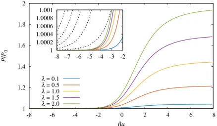
2.1 Result for the pressurePnormalized by the non-interacting counterpartP0that is obtained when attempting a mean-field analysis for the interacting Hamiltonian. The results are shown for a variety of dimensionless couplingsλ, which is related to the bare coupling by λ = √βg. Comparing to the result obtained via HMC in Fig. 3.2, we can see the result is somewhat qualitatively correct within the virial region, but the result is completely wrong for large values of βµ. Inset: A comparison of the mean-field result with the second-order
virial expansion of the pressure (shown as a dashed black line). Mean field fails to correctly quantitatively capture the behavior of the virial region. . . 18 2.2 Rendering of an auxiliary field σ which is of spacetime extent Nx × Nτ = 51×60 at a
given point in its classical trajectory some time after thermalization has occurred. Note that the field is valid only at integer lattice points; the solid planes between such points are for visualization only. . . 24 3.1 Density n, in units of the density of the noninteracting system n0, as a function of the
dimensionless chemical potential βµand couplingλ. From bottom to top, the coupling is λ=0.0,1.0,1.25,1.5, . . . ,2.5,2.75,3.0,3.1,3.2, . . . ,4.0. The dashed line joins the maxima at eachλ. . . 29 3.2 Pressure P, in units of the pressure of the noninteracting system P0, as a function of the
dimensionless chemical potential βµand couplingλ, as obtained by βµintegration of the density. The values ofλshown in this plot are the same as in Fig. 3.1. . . 30 3.3 Isothermal compressibilityκ, in units of the compressibility of the noninteracting systemκ0,
as a function of the dimensionless chemical potential βµand couplingλ, as obtained byβµ differentiation of the density. The values ofλshown in this plot are the same as in Fig. 3.1, but from top to bottom instead. . . 30 3.4 Tan’s contactC scaled by βλT/(2Q1λ2) = πβ2/(2Lλ2) as a function of βµ. The black
line showsCin the absence of interactions. Inset: Zoom-in of the main plot on the region
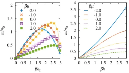
−4.5 ≤ βµ≤ −1.0, also showing the leading-order virial expansion. Both plots show data forλ=0.5,1.0,1.5, . . . ,4.0, which appear from bottom to top. . . 34 4.1 Left: Density as a function of the imaginary chemical potential difference βhI at various
values of βµ. Right: Analytic continuation of the density as a function ofβh. In both plots
the density is an even function about the origin. Both plots are at a dimensionless coupling of λ=1.0, and the physical quantities are plotted in units of the density of the noninteracting, unpolarized system. . . 38 4.2 Left: Magnetization as a function of the imaginary chemical potential difference βhI at
various values ofβµ. Right: Analytic continuation of the magnetization as a function ofβh.
4.3 Left:Tan’s contact as a function of the imaginary chemical potential differenceβhIat various
values of βµfor a dimensionless coupling ofλ = 1.0. C0 is the contact at βh = βµ = 0.
Right: Analytic continuation of the contact as a function of βh at various values of βµ.
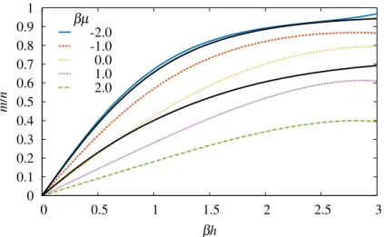
In both plots the contact is an even function about the origin. The curves on the right are color-wise paired by their value of βµ, which coincides with the value on the left (by color code, or from top to bottom). Dashed-dotted lines give the results from a fit of the data to the polynomial-type ansatz (4.10), whereas solid lines result from fits of the data to our Padé-type ansatz (4.8) for the fit functions. . . 39 4.4 Ratio of the magnetization m to the density n as a function of the real-valued βh and
βµ = −2.0,−1.0,0,1.0,2.0. The solid lines show the second-order virial expansion at βµ=−2(top) and -1 (bottom). Note that the virial expansion works well for βµ=−2, but fails dramatically forβµ=−1and above; see Sec. 4.4.1 for details. . . 45 4.5 The magnetic susceptibility χ as a function ofβhat representative values ofβµ, obtained
by taking an analytic derivative of the magnetization with respect to βh. Left: Interacting
case atλ=1. Right: Noninteracting case in the continuum. . . 45
4.6 Density and magnetization at a dimensionless coupling ofλ=1.0in units of the unpolarized, noninteracting densityn0. The solid black lines how the second-order virial expansion for each value of βh. Error bars were estimated by varying the fit parameters by an amount given by the uncertainty in the calculated fits. . . 48 4.7 Left:Tan’s contact as a function of the imaginary chemical potential differenceβhIat various
values of βµfor a dimensionless coupling ofλ = 1.0. C0 is the contact at βh = βµ = 0.
Right: Analytic continuation of the contact as a function of βh at various values of βµ.
In both plots the contact is an even function about the origin. The curves on the right are color-wise paired by their value of βµ, which coincides with the value on the left (by color code, or from top to bottom). Dashed-dotted lines give the results from a fit of the data to the polynomial-type ansatz (4.10), whereas solid lines result from fits of the data to our Padé-type ansatz (4.8) for the fit functions. . . 49 4.8 Comparison of the Monte Carlo results after the analytic continuation, a
next-to-leading-order perturbation theory calculation, and the free gas for the density and the magnetization. Results are displayed in βh = 0.0,0.5,1.0,1.5 and 2.0 in the strongly interacting region βµ >−1. . . 50 5.1 Feynman diagram for the next-to-leading order (NLO) contribution to the grand canonical
partition function. . . 61 5.2 Feynman diagrams for the next-to-next-to-leading order (N2LO) contribution to the grand
canonical partition function. . . 62 5.3 Feynman diagrams for the next-to-next-to-next-to leading order (N3LO) contribution to the
grand canonical partition function. . . 62 5.4 Feynman diagrams for the next-to-next-to-next-to-next-to leading order (N4LO) contribution
to the grand canonical partition function. . . 63 5.5 The perturbative expansion for the grand-canonical partition function aslnZ= P/P0written
5.6 PressurePof the attractive (top) and repulsive (bottom) unpolarized Fermi gas in units of the pressure of the noninteracting system P0, as shown for the dimensionless interaction strengthsλ=0.5, 1.0, 1.5, 2.0, andλ=−0.5, -1.0, -1.5, -2.0 for the attractive and repulsive cases, respectively. The NLO (dashed line), N2LO (dash-dotted line), and N3LO (solid line) results from perturbation theory are displayed for each coupling. The corresponding data points for each attractive coupling are computed using HMC (see Ref. [1]). . . 69 5.7 Densitynof the attractive (top) and repulsive (bottom) unpolarized Fermi gas in units of the
density of the noninteracting systemn0, as shown for the dimensionless interaction strengths λ = 0.5, 1.0, 1.5, 2.0 (attractive), and λ = −0.5, -1.0, -1.5, -2.0 (repulsive). The NLO (dashed line), N2LO (dash-dotted line), and N3LO (solid line) results of perturbation theory are displayed for each coupling and are compared with HMC results (see Ref. [1]) in the attractive case. For both plots, the black diamonds show CL results (RL for the attractive case), regulated withξ =0.1as described in the main text. The statistical uncertainty of the CL results is estimated to be on the order of the size of the symbols, or less, as supported by the smoothness of those results. . . 70 5.8 Densitynof the attractive (top) and repulsive (bottom) unpolarized Fermi gas in units of the
density of the noninteracting systemn0, as shown for the dimensionless interaction strengths λ = 2.5, 3.0, 3.5, 4.0 (attractive), and λ = −2.5, -3.0, -3.5, -4.0 (repulsive). The NLO (dashed line), N2LO (dash-dotted line), and N3LO (solid line) results of perturbation theory are displayed for each coupling and are compared with HMC results (see Ref. [1]) in the attractive case. It is evident that perturbation theory fails miserably at these higher couplings, and competing oscillations set in for the repulsive case. For both plots, the black diamonds show CL results (RL for the attractive case), regulated withξ=0.1as described in the main text. The statistical uncertainty of the CL results is estimated to be on the order of the size of the symbols, or less, as supported by the smoothness of those results. . . 71 5.9 Fifth-order perturbative virial expansion for the pressureP/P0for two attractive and repulsive
couplings. The expansions are shown for which the virial coefficients are computed at NLO (dashed line), N2LO, (dotted line), and N3LO (dash-dotted line). The fully solid line shows the full perturbative calculation of the pressure at N3LO, as shown in Fig. 5.6. Results from HMC data (see Ref. [1]) are displayed as corresponding data points for the attractive couplings. 73 5.10 Plot of the second, third, fourth, fifth, and sixth-order virial coefficients as computed via
Fourier projection under third-order lattice perturbation theory, shown as a function of the dimensionless couplingλ. The plot displays the virial coefficients from the non-interacting limit ofλ=0to the strongly-coupled regime. . . 75 5.11 Reduced class diagram for the C++ implementation of computing the analytic expressions
for perturbative contributions to the grand-canonical partition function. All objects used in the calculation are derived from the SymbolicTerm class, and can be broken into two
categories. The left hand side of the diagram contains expression objects which are con-tainers for pointers to one or moreSymbolicTerminstances (which itself may resolve to an
expression object), and the right hand side of the diagram shows terminal objects which are representations of mathematical objects that appear in the perturbation theory formalism. For brevity, this diagram only displays particular methods and fields discussed further in the text below. In addition, each class typically provides relevant operator overloads to define particular behaviors, as well as overriding implementations of SymbolicTerm::copy()
6.1 The normalized density n/n0, where n0 is the noninteracting result, for λ = −1.0 and βµ=1.6, as a function of the Langevin timetfor several values for the regulating parameter ξ [see Eq. (6.13)]. The result was computed on a spatial lattice ofNx =80and a temporal
lattice of Nτ = 160. For a choice of ξ = 0, where the regulating term is removed, CL tends toward an incorrect value for the density. Whenξ ' 0.1, the additional term provides a restoring force and the stochastic process converges to a different value consistent with perturbation theory. On the other hand, for cases where ξ < 0, the solution diverges, as expected. Each plotted line corresponds to a fixed count of105iterations of performing one integration step of the adaptive stepδt; as such, the length of the line gives an indication as to the computational demand to reach timetfor a givenξ. . . 87 6.2 Plot of the complex quantitye−Sin terms of its magnitudeρand phaseθsuch thate−S = ρeiθ,
for a CL calculation atλ= −1.0andβµ=1.6. Data points are plotted asln(ρ)cos(θ)and ln(ρ)sin(θ) as parametric functions of the Langevin time t. Plots are displayed for four values of the parameter ξ. Note that for ξ = 0, the solution does not converge, but does converge forξ =0.005and0.1. For the case whereξ =−0.1, the result for the densityn/n0 rapidly diverges, as expected [note change in scale fory axis and see Fig. 6.1]. Data points show the locations where samples were taken along the CL trajectory; the shaded areas result from straight lines joining the data points. . . 88 6.3 Histograms of values taken of2 ln(|detM|)over the course of a CL simulation atξ = 0.1
for a few representative values of the couplingλ(shown primarily on the repulsive side and for the strongest coupling) and the chemical potential βµ(shown in the virial and strongly interacting regions). The distributions across parameter values appear approximately log-normal and well behaved, and indicate that the drift force is generally free of singularities. Although the magnitude of the action can vary across parameter space, the variance across field configurations is centered about a well-defined mean. . . 90 6.4 Density equation of staten=n↑+n↓normalized by the non-interacting, unpolarized
coun-terpartn0, for attractive (top) and repulsive (bottom) interactions of strengthλ=±1. Insets:
Zoom in on region βµ > 0 (top) and βµ > 1 (bottom). In all cases, the CL results are shown with colored symbols, iHMC results (from Ref. [2]) appear with black diamonds, perturbative results at third order are shown with solid lines, and virial expansion results appear as dashed lines. . . 94 6.5 Density equation of staten=n↑+n↓normalized by the non-interacting, unpolarized
coun-terpartn0for attractive (top) and repulsive (bottom) interactions of strengthλ=±2. Insets:
Zoom in on region βµ > 0 (top) and βµ > 1 (bottom). The CL results are shown with colored symbols, perturbative results at third order are shown with solid lines, and virial expansion results appear as dashed lines. . . 95 6.6 Density equation of staten=n↑+n↓normalized by the non-interacting, unpolarized
6.7 Spin polarizationm = n↑−n↓ normalized by the non-interacting, unpolarized counterpart
n0for attractive (top) and repulsive (bottom) interactions of strengthλ=±1. The CL results are shown with colored symbols, iHMC results (from Ref. [2]) appear with black diamonds, perturbative results at third order are shown with solid lines, and virial expansion results appear as dashed lines. . . 97 6.8 Spin polarizationm=n↑−n↓normalized by the non-interacting, unpolarized counterpartn0
for attractive (top) and repulsive (bottom) interactions of strengthλ=±2. The CL results are shown with colored symbols, perturbative results at third order are shown with solid lines, and virial expansion results appear as dashed lines. . . 98 6.9 Spin polarizationm=n↑−n↓normalized by the non-interacting, unpolarized counterpartn0
for attractive (top) and repulsive (bottom) interactions of strengthλ=±4. The CL results are shown with colored symbols, perturbative results at third order are shown with solid lines, and virial expansion results appear as dashed lines. . . 99 6.10 Left: Relative difference between the densityn↑+n↓computed via CL (nCL) and the
third-order perturbative resultnPTfor three positive values ofβµ, as a function of the CL timestep tCL. The dashed horizontal line shows wherenCL=nPT. Right: Relative difference between
nCLand the third-order virial expansionnvirialfor three values ofβµof small fugacity, as a function oftCL. The dashed horizontal line shows wherenCL = nvirial. In both plots, the coupling was set toλ= ±1, where solid and open symbols refer to repulsive and attractive couplings, respectively. Error bars represent the statistical error of the CL calculation, and indicate agreement with PT and the virial expansion astCL→0. . . 100 6.11 Architecture of the convolutional neural network. The complex, normalized form of the
fermion matrix is inserted as the input of the convolutional network. Additional information is passed in at an intermediate step through the sequential network, and two output neurons categorize the accuracy of the considered auxiliary field configuration (see main text). . . 102 6.12 Predictions and performance of the trained convolutional neural network shown in Fig. 6.11.
The plots on the left hand side corresponds to the case of attractive interactions whereλ=1, and the right corresponds to repulsive interactions whereλ=−1. Top:Densitynnormalized
by the non-interacting counterpartn0. Values of the density made by the CNN prediction (black squares), CL simulations (green circles), and N3LO reference values (purple triangles) are shown. The red shaded curve indicates the standard deviation of all samples provided by CL, and the blue shaded curve shows the standard deviation of the subset of samples selected by the CNN whose error is estimated to be≤10%. Center: Percentage of the samples across
the training and validation data sets which were correctly classified by the CNN for each value of βµ. Bottom: Fraction of the density samples whose error is≤ 10%for each value of βµ. In all plots, the grey shaded region indicates the values of βµwhose samples were used to train the CNN. . . 105 7.1 Density equation of statennormalized by the non-interacting counterpartn0 for the
spin-balanced attractively interacting Fermi gas in two spatial dimensions as a function of the dimensionless chemical potential βµ. Curves are displayed for five interaction strengths from βB = 0.1 to 3.0. Colored symbols correspond to CL calculations at Nx = 16, and
black diamonds correspond to HMC calculations [3] atNx =19, where both are at β =10.
7.2 Density equation of statennormalized by the non-interacting counterpartn0 for the spin-polarized attractively interacting Fermi gas in two spatial dimensions as a function of the dimensionless chemical potential βµ. Curves are displayed for five polarizations from βh = 0.0to 2.0. Colored symbols correspond to CL calculations at βB = 0.1(top) and
βB = 0.5(bottom) for Nx = 16and β = 10. PT at N2LO (red solid lines) is shown for
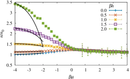
the polarized case, and at N3LO (pink dotted line) for the spin-balanced case. Note that the values ofβhfor each of the PT curves correspond to that of the CL data points from bottom to top. . . 111 7.3 Top: Density of the unpolarized UFG obtained with CL (blue squares), in units of the
noninteracting, unpolarized density n0 as a function of the dimensionless mean chemical potential βµ. Also shown is the third-order virial expansion (dashed line), experimental results of Refs. [4, 5] (red circles), bold diagrammatic Monte Carlo (BDMC) calculations [5] (dark diamonds), and determinantal hybrid Monte Carlo (DHMC) calculations [6] (light diamonds). Bottom: Compressibility κ as derived from the density EOS, in units of its
noninteracting counterpartκ0as a function of the dimensionless pressureP/P0(blue squares). A comparison is made to experimental values [4] (red circles) and the third-order virial expansion (dashed line). Statistical uncertainties for the CL results are on the order of the symbol sizes. The shaded areas indicate the superfluid phase. . . 114 7.4 Densityn=n1+n2of the spin-polarized Fermi gas at unitarity in three spatial dimensions,
normalized by the density of the non-interacting, unpolarized systemn0. Results using CL are shown in colored points for chemical potential asymmetries βh=0.0, 0.4, 0.8, 1.2, 1.6, and 2.0 at a spatial lattice volume ofN3
x =73. The second-order virial expansion is shown in
solid black lines. Additionally, experimental results for the unpolarized system at unitarity are shown in solid red circles (see Ref. [4]). . . 115 7.5 Left: Density of the UFG in units of the noninteracting density, from top to bottom: βh=0
(circles), 0.4 (octagons), 0.8 (hexagons), 1.2 (pentagons), 1.6 (squares), 2.0 (triangles), compared to the third-order virial expansion (dashed lines). Note the colors encode fixed values of βµshown in all panels. Center: Magnetization in units of the interacting density
for the balanced system as a function of βh for several values of βµ. For βµ ≤ −1.0, the third-order virial expansion is shown with dashed lines. Right: Dimensionless magnetic
susceptibilityχ¯Mas a function ofβh(symbols) compared to the corresponding susceptibility
of the free Fermi gas χ¯0
M (dotted lines) at equal chemical potential and asymmetry (color
LIST OF TABLES
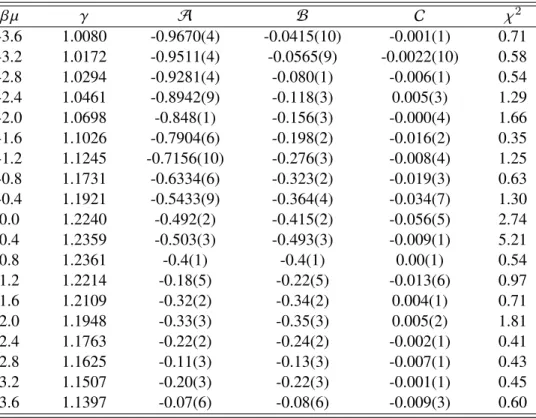
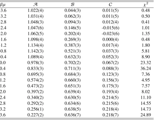
4.1 Fit parameters for the density as they appear in Eq. (4.8) at a constant dimensionless coupling ofλ = 1.0for various values of βµ, as well as the χ2 per degree of freedom for each fit. Note thatγis not a fit parameter (see main text). . . 42 4.2 Fit parameters for the magnetization as they appear in Eq. (4.5) at a constant dimensionless
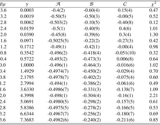
coupling ofλ = 1.0for various values of βµ, as well as the χ2 per degree of freedom for each fit. . . 43 4.3 Fit parameters for the contact as they appear in Eq. (4.8) at a constant dimensionless coupling
ofλ = 1.0for various values of βµ, as well as the χ2 per degree of freedom for each fit. Note thatγis not a fit parameter (see main text). . . 44 5.1 Detail of leading order (NLO), leading order (N2LO), and
next-to-next-to-next-to-leading order (N3LO) contributions (respectively, order A2, A4, and A6) to the grand-canonical partition function Z. The indicated diagram figure refers to the corresponding fully-connected Feynman diagram or product of such diagrams for each con-tribution. The volumeV = NxNτ that appears in all expressions refers to the spacetime
volume of the lattice. The greatest number of loops that appear for each fully-connected dia-gram is also provided. It is implicit in the notation that a momentum-conserving Kronecker delta has been utilized to eliminate momentum sums: one in the case ofS4andS(1)
4 , but two in the case ofS6. . . 64 5.2 Part I detail of next-to-next-to-next-to-next-to (N4LO) contribution (orderA8) to the
grand-canonical partition function Z. The remainder of the N4LO contributions are provided in Table 5.3. All diagrams that appear in this table are disconnected diagrams, and will cancel after the logarithm of the partition function is taken. The indicated diagram figure refers to the corresponding fully-connected Feynman diagram or product of such diagrams for each contribution. The volumeV = NxNτ that appears in all expressions refers to the
spacetime volume of the lattice. The greatest number of loops that appear for each fully-connected diagram is also provided. It is implicit in the notation that a momentum-conserving Kronecker delta has been utilized to eliminate momentum sums. . . 65 5.3 Part II detail of the next-to-next-to-next-to-next-to (N4LO) contribution (order A8) to the
grand-canonical partition functionZ. The first part of the N4LO contributions are provided in Table 5.2. All diagrams that appear in this table are new fully-connected diagrams that appear at this order. The indicated diagram figure refers to the corresponding fully-connected Feynman diagram or product of such diagrams for each contribution. The volumeV =NxNτ
that appears in all expressions refers to the spacetime volume of the lattice. The greatest number of loops that appear for each fully-connected diagram is also provided. It is implicit in the notation that a momentum-conserving Kronecker delta has been utilized to eliminate momentum sums. . . 66 5.4 Results for the second, third, fourth, and fifth-order virial coefficients of the pressure P
[see Eq. (5.50)] at NLO, N2LO, and N3LO for two repulsive and attractive couplings. All coefficients are computed for a spatial lattice size of Nx = 100, β = 8.0, and a temporal
LIST OF ABBREVIATIONS
1D one spatial dimension 2D two spatial dimensions 3D three spatial dimensions CL complex Langevin EOS equation of state FFT fast Fourier transform HMC hybrid Monte Carlo HS Hubbard-Stratonovich NLO next-to-leading order
N2LO next-to-next-to-leading order
N3LO next-to-next-to-next-to-leading order PT perturbation theory
LIST OF SYMBOLS
β inverse temperature µ chemical potential
h chemical potential asymmetry g bare coupling
bn n-th order virial coefficient
z fugacity
λ dimensionless coupling λT thermal de Broglie wavelength
ˆ
N particle number operator ˆ
H Hamiltonian operator ˆ
T kinetic energy operator ˆ
V potential energy operator M fermion matrix
Nx spatial lattice volume
Nτ temporal lattice volume C Tan’s contact
P pressure n density S action
σ Hubbard-Stratonovich auxiliary field π auxiliary momentum field
CHAPTER 1: Introduction
The many-body system, both in the context of classical and quantum physics, has been a long-standing problem in a variety of fields. The classic n-body problem is a gravitational system of orbiting massive bodies according to a pairwise1/rcentral potential, which requires the use of numerical tools to exactly solve the equations of motion beyond the two-body problem [7]. An understanding of the many-body problem in the context of quantum mechanics is crucial to a vast number of physically relevant systems, particularly throughout nuclear and condensed matter physics. Gluons form colorless bound states to produce hadrons, protons and neutrons interact to form nuclei, and electrons live on lattices of ions to provide unique materials, such as graphene. Tackling these challenges proves to be especially fruitful: the study of the quantum-many body problem illuminates the properties of how the universe’s building blocks interact to create the dynamical phenomena around us.
Given this challenge of finding solutions to the quantum many-body problem, the development of numer-ical methods is a crucial pillar to supporting this track of research. Quantum Monte Carlo (QMC) techniques are used across nuclear [8], condensed matter [9], and high-energy physics [10] to nonperturbatively probe the collective behavior of interacting many-body systems in the quantum limit. Extracting quantitative infor-mation about the thermodynamics of these systems is notoriously difficult, or even practically impossible, in particular regimes of interest. For example, systems with a finite chemical potential in the context of quantum chromodynamics (QCD), imbalanced systems of ultracold fermions, and particular kinds of phys-ical interactions pose a significant challenge to QMC methods. The most general roadblock preventing the study of these rich systems is the appearance of the sign and signal-to-noise problems which cause stochastic methods to break down and provide incorrect, inaccurate, or diverging results. At its core, thesign problem
techniques to study many-body systems with limited computational resources are of general interest. The development of new techniques to overcome the sign problem in the context of non-relativistic quantum many-body systems will be the topic of this dissertation.
Section 1.1: Dissertation overview
In the present dissertation, we will focus on the development and testing of novel nonperturbative (stochastic) and semi-analytic perturbative techniques to calculate thermodynamic observables for non-relativistic systems normally plagued by a sign problem. In particular, we choose to study a system of fermions under both attractive and repulsive contact interactions at finite temperature; the variant of the system in one spatial dimension is generally known as the Gaudin-Yang model [12, 13]. The one-dimensional system is studied extensively here in light of benchmarking new techniques, but studies are extended to higher dimensions in the final chapter. The methods we have implemented include extensions to the more conventional hybrid Monte Carlo technique (which is a stochastic method based on the Metropolis-Hastings algorithm), the complex Langevin method (which permits the study of systems where the fermion matrix is complex, but drops the Metropolis algorithm for stochastic noise), and a novel perturbative method performed on the lattice. All of these techniques were used to study thermodynamic quantities of strongly-interacting fermions, including computing the density and pressure equations of state, virial coefficients, the isothermal compressibility, and Tan’s contact. These observables are frequently compared to the virial expansion, which becomes valid in the semiclassical regime. To the best of our knowledge, the results that we have published, including those for repulsively-interacting and spin-polarized systems, are not previously known, even though these can be considered classic many-body condensed matter systems.
The work conducted over the course of the doctoral program for this dissertation has resulted in the following peer-reviewed publications, which form the basis of most of the upcoming chapters.1 A footnote
on the first page of each such chapter indicates the publications it is based upon. Quite often, the text in the dissertation provides additional discussion or details that were not available in the original manuscript.
1. M. D. Hoffman, P. D. Javernick, A. C. Loheac, W. J. Porter, E. R. Anderson, and J. E. Drut,Universality in one-dimensional fermions at finite temperature: Density, pressure, compressibility, and contact,
Physical Review A92, 013631 (2015)
2. Andrew C. Loheac, Jens Braun, Joaquín E. Drut, and Dietrich Roscher,Thermal equation of state of polarized fermions in one dimension via complex chemical potentials, Physical Review A92, 063609
(2015)
3. M. D. Hoffman, A. C. Loheac, W. J. Porter, and J. E. Drut,Thermodynamics of one-dimensional SU(4) and SU(6) fermions with attractive interactions, Physical Review A95, 033602 (2017)
4. Andrew C. Loheac and Joaquín E. Drut, Third-order perturbative lattice and complex Langevin analyses of the finite-temperature equation of state of non-relativistic fermions in one dimension,
Physical Review D95, 094502 (2017)
5. Andrew C. Loheac, Jens Braun and Joaquín E. Drut,Polarized fermions in one dimension: density and polarization from complex Langevin calculations, perturbation theory, and the virial expansion,
Physical Review D98, 054507 (2018)
6. Lukas Rammelmüller, Andrew C. Loheac, Joaquín E. Drut, and Jens Braun, Finite-Temperature Equation of State of Polarized Fermions at Unitarity, Physical Review Letters121, 173001 (2018)
The following article was published during the program, but falls outside the scope of this dissertation: 1. L. Rammelmüller, W. J. Porter, A. C. Loheac, and J. E. Drut,Few-fermion systems in one dimension:
Ground- and excited-state energies and contacts, Physical Review A92, 013631 (2015)
Section 1.2: Why are non-relativistic systems interesting?
Modern QMC techniques are famous for their widespread use in lattice quantum chromodynamics (QCD), where the relativistic field theory of quarks and gluons are placed on a lattice such that they can be studied on a computer. The application of QMC to the non-relativistic counterpart in condensed matter physics is equally important, as non-relativistic systems of fermions and bosons are prevalent in many physical phenomena. A few of the foremost examples include ultracold atomic clouds, which may be controlled via Feshbach resonances and can exhibit interesting phase transitions and superfluid states.
the stochastic evaluation of path integrals is common to both relativistic and nonrelativistic theories, an important distinction between the two formalisms is the construction of differing fermion actions and the computational demand required to work with them. In this context, the study of nonrelativistic systems offers a more tractable challenge to benchmark new numerical algorithms as they are further developed, which can later be transferred to more difficult situations. In the relativistic case, one must be most concerned with maintaining local gauge invariance and consequences of breaking continuous rotational symmetry when discretizing the theory onto a lattice, which leads to introduction of plaquettes and the resulting Wilson gauge action [14]. This naturally leads to the construction of a gauge action, which by itself is a rich yet interesting theory to study. For further reading on QMC techniques for relativistic theories, we point the reader to texts [15, 16] on the subject.
Section 1.3: Brief survey of quantum many-body methods
In addition to the methods to address the sign problem presented in the following chapters, there are of course a whole host of techniques that others have used across the disciplines mentioned above. However, most of these methods are only applicable to particular models or dimensionality, are restricted to a particular regime of parameter space, or are notab initiotechniques, or methods with start from a
well-defined Hamiltonian and systematically proceed without limiting assumptions. Additionally, many more tractable analytical solutions exist for systems at zero temperature (studies of the ground state) compared to systems at finite temperature. Systems in one spatial dimension are generally more soluble by analytic means compared to higher dimensions, if such a technique can be found. We will, however, provide a very brief survey of some of these additional methods for a handful of situations in the present chapter; it should be noted that overview is far from exhaustive.
The classic problem studied in quantum chemistry and condensed matter are properties of quantum systems close to “zero-temperature”, or cases where the ground-state of the system dominate the dynamics of the system. Although this type of analysis can provide many key properties, such as electronic structure and spectroscopy information, and may be sufficient in a wide array of situations, finite temperature can have a drastic effect on the behavior of particular systems.
properties of ferromagnetism. An extension of this method to systems at finite temperature, known as the thermodynamic Bethe Ansatz (TBA) [21] was introduced, but the method results in an infinite tower of coupled partial differential equations that must at some point be truncated, is difficult to work with, and is restricted to one spatial dimension. Nevertheless, it has been applied to a number of models of interest, including a number that are on the lattice [22–24]. Since the Bethe ansatz and its thermodynamic counterpart can, in principle, study a whole host of one-dimensional models, many might consider the 1D interacting system to be solved; however, many such studies remain unexplored which must overcome limitations of this analytic method, particularly for systems at finite temperature. Some of these previously unknown results in one spatial dimension are presented in this dissertation.
Beyond analytic techniques, numerical methods have also been developed to extract properties of systems at zero temperature, such as the ground-state energy of a strongly interacting system. Perhaps the most widely known is the Hartree-Fock method [25], which is applicable to a wide range of many-electron atomic and molecular systems, and is a popular starting point in many quantum chemistry and solid state [26] problems. A number of Monte Carlo methods exist to study systems in the ground state, including diffusion Monte Carlo (DMC), Green’s function Monte Carlo (GFMC) [27] and variational Monte Carlo (VMC) [28], and auxiliary field Monte Carlo (AFMC). These techniques have been used to compute various interesting physical quantities, such as ground-state and low-lying excited state energies of nuclei [29–34], estimates on isospin-mixing matrix elements [34], and the first calculation of the matrix elements for neutrinoless double beta decay for light nuclei [35]; many of these calculations have extraordinary agreement with experiments [8].
These Monte Carlo and other ab initiomethods are capable of studying properties of light nuclei, but
begin to break down as the number of nucleons becomes too large. Density functional theory (DFT) [36– 38], although notab initio, has proved successful in attacking even the largest nuclei, and has recently been
applied to Fermi gases [39]. Mean-field theory is frequently leaned upon whenab initiocalculations become
fermionic theory into one written in terms of bosons. As can be seen, there exists a small zoo of techniques to address studies of interacting many-body quantum system. No single method has risen as superior to all others, as each appears to have their own niche of strengths. New techniques and improvements on old ones constantly appear on the market, with perhaps the most modern additions involving applications of machine learning.
Section 1.4: Experimental counterparts
CHAPTER 2: Foundations of Interacting Quantum Systems
The overarching goal of the work in this dissertation is to study the thermodynamic properties of interacting many-body quantum systems using several different computational approaches. In particular, we often choose to compute equations of state, which although were not previously known for a number of physical systems studied here, help to quickly benchmark and understand the behavior of new methods. These properties at finite temperature are computed from a partition function in the grand-canonical ensemble of the system, which always serves as a starting point for our analysis. The bulk of the analytic work is in rewriting the partition function in a tractable form from which physics can be extracted with reasonable resources. In this chapter, we will overview such a recasting of the partition function in terms of auxiliary fields, and look at well-established Monte Carlo techniques for computing observables stochastically. We will also discuss the so-calledsign problem, which causes Monte Carlo methods to break down for many
systems of interest, and therefore motivates the development of the techniques in this work.
The analytic starting point for computing thermodynamic properties by all the techniques presented in this work is the grand-canonical partition function for each particular system of interest. This partition
function establishes an ensemble of states for a system that is in thermodynamic equilibrium with heat and particle reservoirs. The typical state variables of this ensemble are the temperatureT (which will typically appear in our formulations as the inverse temperature β = 1/kBT, where we take the Boltzmann constant
kB =1), the spatial volumeV, and the chemical potentialµ. For a quantum mechanical system governed by
a HamiltonianH, the grand-canonical partition function is given by a trace over the Boltzmann weights,ˆ
Z(µ,V,T)=Trhe−β(Hˆ−Í
iµiNˆi)i (2.1)
where the sum in the exponent is over any number of particle species with corresponding chemical potentials. Throughout the following chapters, we will consider spin-1/2 fermions in situations where the chemical potentials for spin-up and spin-down flavors are equal (the spin-balanced case), and where µ↑ , µ↓ (the
Section 2.1: Equations of state for noninteracting quantum gases on the lattice
Before moving to computing equations of state for interacting many-body systems, we should first overview a derivation for the pressure and density equations of state for the noninteracting equivalents. These expressions will frequently enter into our analyses later on, as we typically present thermodynamic quantities for interacting systems in units of the noninteracting counterparts.
For the moment, let us consider the simple system of non-relativistic, unpolarized fermions1 on the
lattice; shortly we will extend the result to polarized fermions. The Hamiltonian for a free system is simply given as the kinetic energy,
ˆ H = pˆ
2
2m, Hˆ|ki=k|ki, (2.2)
where the momentum operatorˆpmay be extended to any number of dimensions, and the eigenvalues of the Hamiltonian are labeled ask. Evaluating the partition function in the grand-canonical ensemble for ideal
fermions is straightforward in the occupation number basisnk = {n0,n1,n2, . . .n∞}for each corresponding
single-particle energy levelk. If we now consider spin-1/2fermions which come in two flavors of types
s =↑,↓(such thatµ= µ↑= µ↓andN =N↑+N↓), then for spins,
Zs = ∞ Õ
N=0
Õ
{nk} exp
"
−β Õ
k
nkk−µN ! #
, (2.3)
where the second sum is over the set{nk}that satisfies the total particle numberN, and the sum appearing in the exponent is the total energy of all particles in the system (where we havenk particles of energyk).
By defining the fugacityz≡ eβµ,
Zs =
∞ Õ
N=0
Õ
{nk}
Ö
k
znke−βnkk
(2.4)
for which we may rearrange the various sums in the above to give that
Zs =Ö
k "
Õ
nk
znke−βnkk
#
. (2.5)
For fermions in a given state |ki with energyk, the occupation number of that state may only be either nk =0ornk =1; as such, the partition sum reduces to (the above may be computed for bosons by completing
the geometric sum):
Zs =Ö
k
1+ze−βk. (2.6)
If we consider that the system is placed on a one-dimensional spatial lattice of extentNx, then the product
is taken over the discrete setk = −Nx/2,−Nx/2+1, . . . ,Nx/2−1,Nx/2−1wherek = (2πk/Nx)2/2m.
The total partition function for both spins is of course the product over such spins,Z =Z↑Z↓. In order to
compute thermodynamic observables, we are generally interested inlnZwhich is given by
lnZ =2
Nx/2−1
Õ
k=−Nx/2 ln
"
1+zexp −β 2m
2πk Nx
2! #
. (2.7)
The factor of two in front of the sum arises from the fact that the energy and chemical potential contributions to the for the second spin degree of freedom may be inserted additively in the exponential weight. Additionally, note that in future references to this expression, we will generally always set the fermion massm =1. The noninteracting pressureP0is directly related tolnZ,
P0 = 2 βNd
x
Nx/2−1
Õ
k=−Nx/2 ln
"
1+zexp −β 2m
2πk Nx
2! #
, (2.8)
(whereNd
x is the spatiald-dimensional volume), and the noninteracting densityn0is related by a derivative
with respect to µ,
n0 = ∂∂(βµ)lnZ = 2 Nd
x
Nx/2−1
Õ
k=−Nx/2
1
1+zexp
β 2m
h
2πk Nx
i2
. (2.9)
P0λ3
T =
√
16πI0(z)whereλT ≡√2πβis the thermal de Broglie wavelength and
I0(z)=
∫ ∞
−∞
dx ln(1+ze−x2). (2.10)
Correspondingly, the density in the continuum limit is related toI0(z)by
n0λT = √2z
π ∂I0(z)
∂z . (2.11)
We will use these expressions for the noninteracting system in cases where a Monte Carlo calculation demonstrates convergence to the continuum limit. In the case of a two-component polarized gas, for which we will analyze the interacting case in this thesis, we modify the chemical potential for one species by a differencehsuch thatµ↑ = µ¯+handµ↓ = µ¯−h, where µ¯is the average chemical potential of the system,
¯
µ=(µ↑+µ↓)/2. By modifying the above derivation, it is straightforward to see that for the pressureP0,
P0 = 1 Nd
x ©
« Nx/2−1
Õ
k=−Nx/2
ln(1+ek−µ¯−h)ª ®
¬ ©
« Nx/2−1
Õ
k=−Nx/2
ln(1+ek−µ¯+h)ª ®
¬
(2.12)
wherek =2πk/Nx; the density for the polarized case still follows from Eq. (2.11). Section 2.2: Auxiliary field representation of the partition function
In order to study the systems we are interested in using a stochastic technique, we must rewrite the grand-canonical partition function in a form that is tractable; namely, we must decompose the two-body interaction into a sum over one-body operators. We perform this change by the means of a Hubbard-Stratonovich transformation, where we introduce an auxiliary fieldσwhich exists in the spatial and temporal dimensions
of the system. We will provide an overview of this transformation in the following section.
Recall that the grand-canonical partition function for a general system of quantum particles is given by the trace over Boltzmann weights,
Z=Trhe−β(H−ˆ µNˆ)i, (2.13)
whereβ =1/kBT,Hˆ is the Hamiltonian operator, µis the chemical potential, andNˆis the particle number
non-trivial task for the vast majority of interesting systems. In the case of interacting systems, the kinetic and potential energy operators do not commute ([T,ˆ Vˆ] , 0) which implies eachN-particle subspace must individually be diagonalized. In addition, the size of the applicable single-particle basis and the number of degrees of freedom are typically very large. As such, most studies of quantum many-body systems turn to alternate routes that rewrites the problem in a form that is tractable by analytical or numerical means. In the majority of the approaches we use in the following work, we choose the rewrite the grand-canonical partition function as a path integral over a continuously-varying auxiliary field using a Hubbard-Stratonovich transformation.
Our natural goal for this problem is not necessarily to compute the partition functionZitself per se, but rather to computephysical observablesfor the Hamiltonian of interest, which can analytically be computed
by taking derivatives of the partition function with respect to various sources, e.g. for an inserted source j where jOˆis added to the Hamiltonian,
hOˆi= δlnZ(j) δj
j=0 = 1
Z δZ(j)
δj
j=0
, (2.14)
or one may follow the more conventional route of numerically computing the expectation value of some observableOˆvia,
hOˆi= 1 ZTr
h
ˆ
Oe−β(Hˆ−µNˆ)
i
. (2.15)
However, computing this in a naive manner by taking a complete trace over the Fock space is generally an intractable task; our present goal is to rewrite the problem in a form such that hOiˆ can be reasonably computed. The first step is to consider the Trotter-Suzuki factorization [64] of thetransfer matrixTβ ≡e−βHˆ,
such that we discretize imaginary time (which is named as such if we considerit →τ),
β=τNτ (2.16)
proceed with the approximation
e−τHˆ =e−τTˆ/2e−τVˆe−τTˆ/2+O(τ3), (2.17)
which we truncate to orderτ2under the requirement thatτis made appropriately small. 2.2.1: Hubbard-Stratonovich transformation for contact interactions
To proceed reformulating our problem of computing observables in a tractable form, we must specify the form of the Hamiltonian of interest. For all of the work developed here, we will study a system of fermions with zero-range contact interactions such that for a two-component system,
ˆ H =
ˆ p2
↑+pˆ
2
↓
2 −g
Õ
x
ˆ
nx,↑ˆnx,↓ (2.18)
wherepˆs are operators in momentum space for the subspace of components, andnˆx,s are density operators
for the componentsat the spatial lattice pointx. The density operators may be expressed in terms of creation and annihilation operators asnˆs = ψˆs†ψˆs. When combined with a non-relativistic formalism on a lattice in
one spatial dimension, this system is known as the Gaudin-Yang model [12, 13].
We will consider a transformation of the partition function for this Hamiltonian to one where the exponential of the two-body operatorVˆis written as a field integral over a one-body operator in the presence of all possible external fields,
e−τVˆ =
∫
Dσ exp(−τVextˆ [σ]). (2.19)
To proceed further explicitly we must specify the form of the interaction potentialV; here we will specifyˆ azero-range contact interactionwhich will become the focus for the rest of the dissertation. Let us formally
specify the interaction matrix as
ˆ
V =−gÕ
j
ˆ
n↑,xnˆ↓,x (2.20)
where the real constantgis thebare couplingwhich specifies the strength of the interaction, and the particle
number operator is againnˆs,x =ψs†,xψs,x. In one spatial dimension, the bare coupling is inversely proportional
used for physical systems by means of Lüscher’s formula [65–67], where the two-body energy spectrum is studied in a finite but continuous volume. For instance, in three spatial dimensions, the limit of low-energy scattering gives for momentumpand phase shiftδ,
pcotδ(p)=−1 a +
1 2reffp
2+O(p4) (2.21)
where reff is the effective interaction range and a is the scattering length; the right hand side is a series expansion in even powers of p [68]. In a finite box of width L with periodic boundary conditions, the scattering phase shift is related to the momentum by [69]:
pcotδ(p)= 1
πLΛlim→∞SΛ(η) (2.22)
whereΛis the ultraviolet cutoff (defined on the lattice by the lattice spacing`, and in the continuumλ→ ∞), η= pL/2π, and
SΛ(η)=
Õ
n
Θ(Λ2−n2)
n2−η2 −4πΛ. (2.23)
Note that hereΘ(x)is the Heaviside step function, andnis a vector of integers labeling the energy eigenstates; the sum is over all such states. A solution of the two-body energy spectrum En = p2n/2mon the lattice
provides the effective range expansion for sufficiently small energies. The bare couplinggmay therefore be connected to the constants appearing the expansion ofpcotδ(p)via a solution of the scattering states for a single body in an external potential.
The ultimate goal of the Hubbard-Stratonovich transformation is to rewrite the interactionVˆin terms of a path integral over decoupled one-body operators that are more easily handled. There are multiple ways of writing a solution. The first step is to exactly state that (by noting that for fermionsˆn2 =ˆn),
exp(τgˆn↑,xnˆ↓,x)=1+(eτg−1)ˆn↑,xnˆ↓,x, (2.24)
for a continuous and compact transformation,
exp(τgˆn↑,xnˆ↓,j)=
∫ π
−π
dσ
2π(1+Anˆ↑,xsinσ)(1+Aˆn↓,xsinσ). (2.25)
Notice that after contracting σ in Eq. (2.25) we recover Eq. (2.24); in a sense, this method is simply a rewriting of the interaction, but determining transformations for other interactions is generally nontrivial. This result also alludes to our first piece of evidence for the sign problem in terms of this system. In the case whereg< 0, where we are in the regime of a repulsive interaction,Abecomes complex, and as we will observe later, the probability measure for our Monte Carlo method becomes ill-defined.
To construct the full Hamiltonian, we should take a product of Eq. (2.25) over all lattice points (recall thatVˆis written in terms of a spatial sum),
e−τVˆ = Ö x
eτgn↑ˆ,xˆn↓,x (2.26)
= Ö
x
∫ π
−π
dσ
2π[1+ Aˆn↑,xsinσt(x)][1+Aˆn↓,xsinσt(x)] (2.27)
where here we have explicitly noted that the matrix elements ofσare indexed by both space and imaginary time. Additionally, we must include the proper kinetic energy operator, noting that it is composed as a sum of operators for each component,Tˆ=Tˆ↑+Tˆ↓, and therefore,
e−τ(Tˆ+Vˆ)
= e−τTˆ/2 Ö
x
∫ π
−π
dσ
2π[1+Aˆn↑,xsinσt(x)][1+Aˆn↓,xsinσt(x)] !
e−τTˆ/2 (2.28)
= Ö
x
∫ π
−π
dσ 2πe
−τT↑ˆ/2[1+Anˆ
↑,xsinσt(x)]e−τ
ˆ
T↑/2 ×
e−τT↓ˆ/2[1+Aˆn
↓,xsinσt(x)]e−τ
ˆ
T↓/2. (2.29)
Here we will define an operator that in generality appears for each components, or flavor, in the system,
ˆ
Us(σ) ≡e−τTˆs/2[1+ Aˆn
s,xsinσt(x)]e−τ
ˆ
Ts/2, (2.30)
giving that
e−τHˆ =Ö
x
∫ π
−π
dσ
The full Boltzmann weight for this system is given by the product of the above right hand side over all points in imaginary time,
e−βHˆ = Nτ
Ö
t Nx
Ö
x
∫ π
−π
dσ
2π Uˆ↑(σ)Uˆ↓(σ), (2.32)
where we may formally define the transfer matrix of a single component as a product ofU over all such points,
Ts(σ)=
Nτ
Ö
t
Us(σ). (2.33)
We additionally define the path integral operator
∫
Dσ=Ö
x
∫ π
−π
dσt(x)
2π , (2.34)
such that
e−βHˆ =
∫
DσTˆ↑(σ)Tˆ↓(σ), (2.35)
where after taking a trace over the Boltzmann weights,
Z=
∫
DσTr[T↑(σ)T↓(σ)], (2.36)
which can further shown to be written as
Z=
∫
Dσdet2(1+zU[σ]), (2.37)
wherez= exp(βµ). This form of the partition function, where the size of the matrix that is an argument to the determinant is of sizeNd
x ×Nxd(rather than the full extent of spacetime), is known as theBSS formalism,
To see how the trace is recast as a determinant, first note that the proof relies on the statistics of fermions; an analogous but different result which contains the inverse of the fermion determinant can be obtained for bosons. Recall that the operators that appear inU[σ]are of the formexp(−τTˆ)andexp(−τVˆ). Therefore, for a generic operator Mi j written in the occupation number basis (for whicha†andaare the creation and
annihilation operators, respectively), consider its exponential such that we want to show
Tr
"
expÕ
i,j
a† iMi jaj
#
=det1+eM
. (2.38)
If M is transformed to a diagonal basis where for a unitary transformationU, M = U†DU and b = Ua, b† =a†U†, then
Õ
i,j
a†
iMi jaj= Õ
k
b†
kDkbk = Õ
k
Dknk, (2.39)
wherenk is the occupation number of statek. Sincebk,b†k obeys the same fermion commutation relations
asak,ak†under the unitary transformation, the trace over Fock space will give onlynk =0and 1. As such,
Tr
"
expÕ
i,j
a† iMi jaj
#
=Ö
k Õ
nk=0,1
eDknk =Ö
k
(1+eDk)=det(1+eM), (2.40)
where the last equality is made by the fact that the product is taken over all eigenvalues of M, which is equivalent to the determinant. A similar proof can be shown for a product of operators,
Tr
" Ö
i
ea†A
ia
#
=det 1+Ö
i
eAi
!
, (2.41)
from which Eq. (2.37) can be shown to hold.
Section 2.3: Difficulty of direct linear algebra and mean field approaches
is a high-order polynomial – clearly such a goal would be fruitless. Finding such roots numerically are known to be sensitive to accumulation of error, particularly when the system is ill-conditioned, e.g. a significant number eigenvalues are close to and may lie on either side of zero. In this sense, it may be difficult to even have enough precision to accurately determine the signs of eigenvalues, which are critical to reasonably computing quantities of the partition function. However, highly-efficient software packages which perform exact diagonalization methods [71] do exist, but are generally not an appropriate choice for studying strongly-interacting systems at finite temperature. In this sense, we choose to exchange the problem of explicitly working with a large number of particles for high-dimensional integrals which are evaluated stochastically.
Another conventional approach to probe analytically intractable systems is via mean field, but it is generally known that these kinds of techniques are unable to capture important fluctuations which contribute to the thermodynamics. Nevertheless, let’s take a very brief look at this method and see how it fails. We will simply attempt to compute the pressureP/P0 of a weakly-interacting system in one spatial dimension, whereP0refers to the pressure of the non-interacting counterpart. Mean field approaches generally improve in higher dimensions, so the 1D system is in a way a “worst-case” scenario for this type of analysis. The Hamiltonian can be built by taking advantage of the Fourier transform, where we define Hˆ = Tˆ+V. Theˆ kinetic energy operatorTˆcan be constructed as a diagonal matrix in momentum space, where the elements Tnare given by (note that the fugacityzis absorbed into these matrix elements):
Tn=
p2
n
2 −µ , pn= 2πn
L (2.42)
where the extent of the one-dimensional lattice is ofLsites. The potential energy operatorVˆfor an attractive contact interaction controlled by the coupling strengthg is correspondingly diagonal in coordinate space, where in this mean-field approach we simply take
hVˆi=−gˆn↑(x)nˆ↓(x). (2.43)
Herenˆs(x) corresponds to the density of the spin-1/2free gas wherenˆ↑ = ˆn↓. The full Hamiltonian can
therefore be constructed in coordinate space via
ˆ
1 1.2 1.4 1.6 1.8 2
-8 -6 -4 -2 0 2 4 6 8
P
/
P0
βµ λ = 0.1
λ = 0.5 λ = 1.0 λ = 1.5 λ = 2.0 1 1.0002 1.0004 1.0006 1.0008 1.001
-8 -7 -6 -5 -4 -3 -2
Figure 2.1: Result for the pressurePnormalized by the non-interacting counterpartP0that is obtained when attempting a mean-field analysis for the interacting Hamiltonian. The results are shown for a variety of dimensionless couplingsλ, which is related to the bare coupling byλ=√βg. Comparing to the result obtained via HMC in Fig. 3.2, we can see the result is somewhat qualitatively correct within the virial region, but the result is completely wrong for large values ofβµ.Inset:A comparison of the mean-field result with the second-order virial expansion of the pressure (shown as a dashed black line). Mean field fails to correctly quantitatively capture the behavior of the virial region.
whereUis the Fourier transform matrix. We must therefore compute the eigenvaluesk for the interacting
HamiltonianH. An understanding of the relative bounds on the error of this operation may be obtained from thecondition number, which provides an estimate of the error in the solution vector x®based on the error in input vector ®yfor the linear systemAx®= y. Here we define the condition number® κ ≡ ||A−1|| ||A||, where a small condition number (κ∼1) indicatesAis well-conditioned, and a large condition number will denote that it is ill-conditioned [72]. Depending on the choice ofµ, we find thatκ∼102−105, which confirms our suspicion that accurately extracting the spectrum could be a challenge. Indeed, when we attempt to compute the pressure from the interacting Hamiltonian for small choices ofg, the result is incorrect compared to a variety of other methods developed throughout this dissertation; although, this limitation is of course due to the mean-field approach in addition to any numerical challenge. Fig. 2.1 shows the result for the pressure using mean-field approach for the one-dimensional system on a lattice size of Nx = 61 and temperature of
β=8. Although the results for the regime ofβµ <0are somewhat qualitatively correct, a comparison with the second-order virial expansion (see inset) indicates that the result is not accurate. More importantly, this mean field completely fails to capture the physics as the temperature is lowered toward large values of βµ where quantum mechanical effects dominate; the pressureP/P0should tend back toward the non-interacting value in this limit. Varying the lattice size Nx and temperature β does not improve this behavior by a
Section 2.4: Finite-temperature determinantal Monte Carlo
Since we know that more straightforward approaches will not work for our studies of the systems we are interested in, we will turn to introducing the foundation for Monte Carlo techniques we use throughout this dissertation. All Monte Carlo techniques, in one form or another, use algorithms that rely on random numbers to study a problem of interest. As a small example, one may estimate the value ofπusing a simple Monte Carlo program. Consider a circle of radius a inscribed inside a square whose side length is 2a. The program can choose N coordinate points(x,y) from a uniform distribution [such that x,y ∈ (−a,a)]. If k is the number of points that fall inside the circle, than approximately π = 4k/N. As N → ∞, this approximation will improve. As a more relevant example of a Monte Carlo algorithm to this work, consider that we are attempting to numerically estimate the value of the integral of a one-dimensional function f(x) over the domain(a,b), which may not necessarily be easily determined analytically. If we choose a suitable
weight functionor probability distributionp(x)we can rewrite the integral as an expectation value:
∫ b
a
f(x)dx =
∫ b
a
f(x)
p(x)p(x)dx =
f
(x) p(x)
. (2.45)
We can approximate the value of this integral by randomly sampling N values over the domain of x according to the probability distribution p(x), and appropriately summing over all samples taken. The choice of how to properly select a set ofxithat will well-represent the integral being taken is a delicate one.
Deciding on an algorithm to perform this sampling may be straightforward for a one-dimensional integral, but in the case of the many-body systems we will be looking at over the next several chapters, the integral we are attempting to estimate (the grand-canonical partition function, which is a path integral over the auxiliary field) has an incredible number of dimensions, which makes this issue drastically more complicated. In the remainder of this chapter, we will discuss the Monte Carlo sampling techniques we use for the quantum many-body problem.
becomes impossible since the number of configurations scales exponentially with the spacetime volume; for instance, for a discrete field that takes on one of two states and is of a spacetime dimension Nd
x ×Nτ,
the number of configurations is2Nd
xNτ. As is commonly seen in statistical mechanics, the vast majority of these configurations contribute negligibly to the dynamics of the system, and in reality, to study the relevant physics, we need only to visit the important contributions to the partition function. In order to do so in practice, we need to construct an algorithm which is capable of sampling such field configurations. In this section, we will discuss aspects of quantum Monte Carlo algorithms which serves as the foundation of stochastic calculations seen in this thesis.
When adding a source term to the Hamiltonian which contains the observable we wish to compute [see Eq. (2.14)], and take a derivative oflnZto computehOˆi, if the partition function is written as a path integral
Z=
∫
DσP(σ), (2.46)
we can arrive at something of the form
hOˆi= 1 Z
∫
DσP(σ)Oˆ(σ). (2.47)
We can identifyP(σ)as a probability measure that will govern our Monte Carlo simulation viaimportance sampling; in the case of fermionic systems, this probability measure will be given by a product of fermion
determinants, as derived in a previous section. If we are given a total ofNσsamples of the auxiliary fieldσ that obey such a probability measure, than we can state that by a Monte Carlo calculation over a discretized field,
hOˆi= 1 Nσ
Õ
{σ}
ˆ
O(σ), (2.48)
whose measurement has an uncertainty of orderO(1/√Nσ)given independent samples. At this point, in order to compute an observable from the partition function we must design an efficient algorithm that samples the probability distribution with particular properties, such as decorrelation, reproducibility, ergodicity, and detailed balance. The Metropolis-Hastings algorithmsatisfies these mathematical underpinnings that
sign problem. In the case of the complex Langevin method, the Metropolis accept-reject step is replaced with the use of a stochastic noise term that is inserted in the action.
The Metropolis-Hastings algorithm produces a Markov chain of statesσthat follows a particular prob-ability (or weight) distribution. The algorithm defines a method of either accepting a proposed move to the next state in the Markov chain, or rejecting it, based on the probability of a system being in the proposed state relative to the current one. In the conventional description of the algorithm [73, 74], if a system in state s is proposed to move to a new stater, the total energies of each stateEs andEr and the energy difference ∆Eare calculated. The proposed step is automaticallyacceptedif∆E <0, otherwise, if∆E >0we choose a random numberR∈ [0,1], where
if
R<exp(−β∆E) accept the proposed state R>exp(−β∆E) reject the proposed state
(2.49)
In this manner, the algorithm can be shown to sample the states of higher probability for a given system. Note that if a proposed state is rejected, the current state is entered as the next state in the chain; that is, the attempt is not simply discarded from the Monte Carlo simulation. In the case of determinantal Monte Carlo, β∆E in the Metropolis algorithm is replaced by anactionin Euclidean time, −S = ln(det2M) (or the equivalent appropriate fermion determinants for a system of study). Therefore, in the context of QMC, the partition function must generally be written in the path-integral form
Z=
∫
Dσ(x, τ)e−S[σ(x,τ)], (2.50)
where one may say we have integrated out the fermionic degrees of freedom and are left only with a path integral over a scalar field. In hybrid Monte Carlo, which we discuss next, we introduce a second auxiliary field that greatly increases the efficiency of the Metropolis sampling algorithm.
2.4.1: Hybrid quantum Monte Carlo