Zhang_unc_0153D_16583.pdf

(1)

INDEX POLICIES FOR PATIENT SCHEDULING AND ATM REPLENISHMENT

Yu Zhang

A dissertation submitted to the faculty at the University of North Carolina at Chapel Hill in partial fulfillment of the requirements for the degree of Doctor of Philosophy in the

Department of Statistics and Operations Research.

Chapel Hill 2016

Approved by: Vidyadhar Kulkarni Nilay Argon

Jayashankar Swaminathan Quoc Tran-Dinh

(2)

c 2016 Yu Zhang

(3)

ABSTRACT

YU ZHANG: INDEX POLICIES FOR PATIENT SCHEDULING AND ATM REPLENISHMENT

(Under the direction of Vidyadhar Kulkarni)

Markov Decision Processes (MDP) are one of the most commonly used stochastic mod-els to solve sequential decision making problems. The optimal solution to many real-world problems cannot be achieved due to the curse of dimensionality. It is common to use a heuris-tic policy called the index policy, which is obtained by applying one-step policy improvement to a simple initial policy. The index policy performs close to the optimal policy and is eas-ily implementable, which makes it attractive to use in practice. In this dissertation, we first introduce the background information on MDP and index policies in Chapter 1. We then study their applications in two problems: the appointment scheduling problem with patient preferences, and the automated teller machine (ATM) replenishment problem.

(4)

(5)

ACKNOWLEDGMENTS

I want to express my deepest gratitude to my advisor, Professor Vidyadhar Kulkarni, for his teaching, guiding, supporting, and encouraging me during the past five years. I feel extremely fortunate to have him as my advisor. Learning from him and working with him made my doctoral study an enjoyable and rewarding experience. He not only taught me how to translate a real-world problem into a research project and build a mathematical model to solve it, but also how to communicate these ideas to others effectively. He helped me grow and improve myself continuously. My gratefulness for numerous efforts he made for me is beyond words.

I also want to extend my appreciation to other committee members: Professor Nilay Ar-gon, Professor Jayashankar Swaminathan, Professor Quoc Tran-Dinh, and Professor Serhan Ziya. In particular, I am grateful to have taken Professor Nilay Argon’s courses on Discrete Event Simulation and Markov Decision Processes and Professor Serhan Ziya’s course on Design and Control of Queueing Systems. Without their effort explaining these complicated subjects in a clear and engaging way, I cannot leverage these useful methods in my research. I am also grateful to Professor Jayashankar Swaminathan and Professor Quoc Tran-Dinh for their insightful comments on my research.

(6)

the formulation of the problem.

(7)

TABLE OF CONTENTS

LIST OF TABLES . . . ix

LIST OF FIGURES . . . xi

1 Markov Decision Processes and Index Policies: Background. . . 1

2 Appointment Scheduling with Patient Preference . . . 6

2.1 Introduction . . . 6

2.2 Literature Review . . . 9

2.3 Base Model . . . 11

2.4 Structural Properties of Optimal Policy . . . 19

2.4.1 Numerical Illustration . . . 23

2.5 Heuristic Policies . . . 26

2.5.1 Shortest-Queue Policy (SQ) . . . 26

2.5.2 Randomized Policy (RP) . . . 28

2.5.3 Index Policy . . . 30

2.6 Numerical Study . . . 35

2.7 Extension of the Base Model: Rejection is Allowed . . . 40

2.7.1 Optimality Equation . . . 40

2.7.2 Structural Properties . . . 42

2.7.3 Numerical Illustration . . . 67

(8)

2.8.1 General Framework and A Simple Case . . . 69

2.8.2 Three-Day Appointment Scheduling . . . 75

2.8.3 Two Variants of Index Policy . . . 81

2.9 Conclusions . . . 86

3 Automated Teller Machines Replenishment Policies . . . 87

3.1 Introduction . . . 87

3.2 Literature Review . . . 91

3.3 Model Description . . . 94

3.4 Single-ATM Problem . . . 100

3.5 Additive-Replenishment-Cost Problem . . . 104

3.6 Structural Properties of Optimal Policy . . . 107

3.7 Heuristic Policies . . . 116

3.7.1 (s, M)Policy (SP) . . . 117

3.7.2 Index Policy (IP) . . . 118

3.8 Numerical Experiments . . . 131

3.8.1 Comparison of IP, SP and OP in Two- and Three-ATM Case . . . 132

3.8.2 Comparison of OP and IP in Additive-Cost Multi-ATM Case . . . 136

3.8.3 Comparison of IP and SP in Submodular-Cost Multi-ATM Case . . . 137

3.9 Real-world Applications . . . 142

3.9.1 Statistical Analysis . . . 143

3.9.2 Parameter Estimation . . . 146

3.9.3 Numerical Study . . . 148

3.9.4 Recommendations . . . 150

3.10 Summary and Future Work . . . 150

(9)

LIST OF TABLES

2.1 j∗(i)andi∗(j)with parametersα= ₁₆15, p1 = 0.1, p2 = 0.1, p12 = 0.8. . . 26

2.2 The values ofρ1givenp1andp2. . . 37

2.3 Long-run average cost under four different policies. . . 39

2.4 Relative efficiencies assuming that on average 15 patients arrive per day. . . 40

2.5 The values ofρ1, ρ2under differentp1, p2. . . 73

2.6 The 95% CI ofimp(IP,SP)(in percentage) whenτ = 15. . . 75

2.9 The 95% CI ofimp(IP,SP)(in percentage) for Negative Binomial. . . 77

2.10 The 95% CI ofimp(IP,SP)(in percentage) for Poisson. . . 77

2.11 The 95% CI for long-run average whenp1 = 0.4, p2 = 0.4, p3 = 0.2. . . 78

2.12 The 95% CI ofimp(PIP,SP)(in percentage) for Poisson(15) arrivals. . . 79

2.15 Comparisons among IP, IPFD, IPEA whenτ = 15. . . 83

2.18 Comparisons among IP, IPFD, IPEA for Poisson(15). . . 84

3.1 Stock-out costs: M = 50 . . . 134

3.2 Stock-out costs: M = 30 . . . 134

(10)

(11)

LIST OF FIGURES

2.1 The cost functionc(x) = E[F(Bin(x, p))]withF as defined in Equation (2.8). . . 25

2.2 The optimal policy for type-12 patients. . . 27

2.3 The regions classified based on the system states. . . 43

2.4 The optimal policy for type-12 patients when the rejection option is available. . . 68

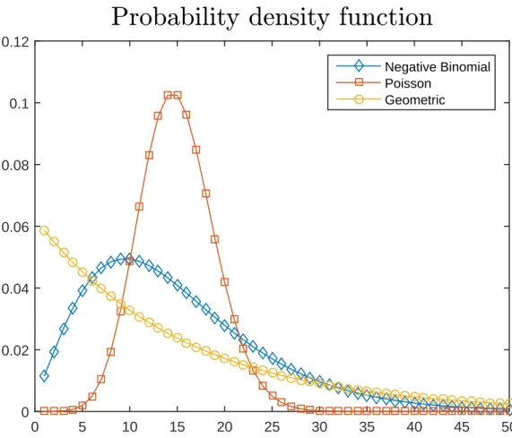
2.5 The comparison among probability density functions . . . 78

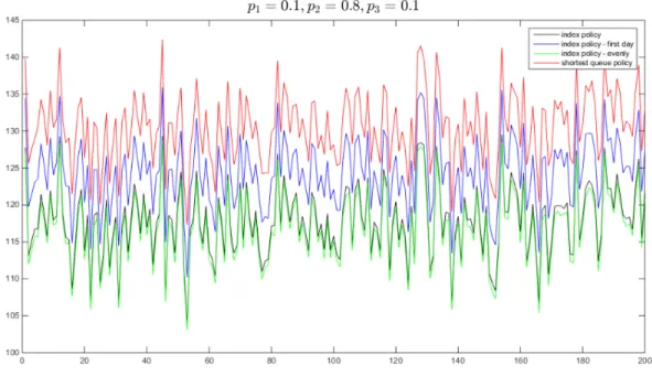
2.6 The comparisons among IP, IPFD, IPEA, and SP. . . 82

3.1 Relationship between service level and stock-out cost . . . 104

3.2 The state-dependent decisions under the optimal policy . . . 114

3.3 The decisions on ATM 1 . . . 115

3.4 The decisions on ATM 2 . . . 116

3.5 The greedy algorithm to find replenishment setA∗ . . . 126

3.6 Long-run average cost . . . 140

3.7 Fraction of stock-out days . . . 141

3.8 Demand vs Date . . . 143

3.9 Demand vs Day of Week . . . 144

(12)

CHAPTER 1: Markov Decision Processes and Index Policies: Background

In this doctoral dissertation, we plan to use Markov Decision Processes and index policies to model and analyze two real-world problems. In this chapter, we collect the background information on Markov Decision Processes (MDP) and the index policies.

MDP is a tool to study sequential decision making problem. (Puterman, 2014) is an excellent reference on this subject. An MDP has five elements: decision epochs, a state space, an action space, transition probabilities and costs. A decision epoch is the point of time when a decision is made. LetXn be the system state at the decision epochn. SupposeXn ∈ S

for alln ≥ 0. We call S a state space. LetAn be the action taken at the decision epochn.

SupposeAn ∈A for alln≥ 0. We callA an action space. The process{(Xn, An), n≥ 0}

is called an MDP if

P(Xn+1 =j|Xn=i, An=a, Xn−1, ..., X1, X0, An−1, ..., A1, A0) = pij(a),

for all n ≥ 0, i, j ∈ S, a ∈ A. We call pij(a)transition probabilities. Let c(i, a) be the

expected cost incurred if actionais chosen in stateiat any timen≥0.

(13)

define (assuming the limit exists)

gπ(i) = lim N→∞

1

N+ 1E π

" _N X

n=0

c(Xn, An)

X0 =i

#

.

We callgπ₍_i₎_{the long-run average cost of following the policy}_{π. Let}

g∗(i) = inf π g

π

(i), ∀i∈S.

If there is a policyπ∗ that achieves this infimum, it is called the average-cost optimal policy. Thus an optimal policy (if it exists) satisfies

gπ∗(i) = g∗(i), ∀i∈S.

Now we discuss when such an optimal policy exists and how to compute it. Define

vn+1(i) = min

a∈A{c(i, a) +

X

j∈S

pij(a)vn(j)}, (1.1)

for alli∈Sandn≥0, wherev0(i) = 0alli∈S. We can interpretvn(i)as the optimal total

expected cost incurred over thendays starting from statei. It is known (see (Tijms, 2003)) thatvn(i)is asymptotically linear innwith slopeg and intercepth(i). We can write

(14)

h(·)is called the bias function. It is known (see (Tijms, 2003)) that g and h(·) satisfy the Bellman equation

h(i) +g = min

a∈_A{c(i, a) +

X

j∈S

pij(a)h(j)}, (1.3)

It is also known (see (Tijms, 2003)) that if Equation (1.3) has a solution, then we can use it to compute the optimal decision as follows. Define

a(i) = arg min

a∈_A{c(i, a) +

X

j∈S

pij(a)h(j)}, ∀i∈S. (1.4)

The standard theory of dynamic programming shows that the Markovian policy that chooses action a(i) in statei is optimal. It is known (see (Tijms, 2003)) that Equation (1.3) has a solution if the MDP is unichain, that is, for each stationary policy the associated Markov chain has no two disjoint closed sets. This fact is formally stated in the next theorem.

Theorem 1. If an MDP is unichain, then Equation 1.3 has a solution.

If Equation 1.3 has a solution, we can solve it by the iterative method in Equation (1.1). We restate Theorem 6.6.1 of (Tijms, 2003) in the theorem below, which allows us to use the recursion in Equation (1.1) to computeg andh(·).

Theorem 2. For any statei, we have

h(i)−h(0) = lim

(15)

and

g = lim n→∞

vn(i)

n . (1.6)

Furthermore,

min

i∈S{vn(i)−vn−1(i)} ≤g ≤maxi∈S {vn(i)−vn−1(i)} (1.7)

However, solving the optimality equation is intractable when the state space and action space are large. Hence, we develop heuristic policies which perform well. One such policy is called the index policy, which we define below.

Suppose the MDP is unichain. Letπbe a given initial policy. Then there exists a solution gπ _{and a bias function}_hπ _{that satisfy}

hπ(i) +gπ = min

a∈_A{c(i, a) +

X

j∈S

pij(a)hπ(j)}.

Now consider a policyπˆthat chooses the actionˆain statei, where

ˆ

a∈arg min

a {r(i, a) + X

j∈S

pij(a)hπ(j)}.

(16)

Theorem 3.

gˆπ ≤gπ.

and ifgˆπ ₌_gπ_{, then}_ˆ_π_{is the average-cost optimal policy.}

Suppose we can construct a functionf :S×A →_Rsuch that

arg min

a f(i, a)⊂arg mina {r(i, a) + X

j∈S

pij(a)hπ(j)}.

The functionf is called an index function and the policyπˆis called an index policy using the index functionf. It has been observed that the index policyπˆprovides a tractable heuristic policy, especially if the initial policyπis chosen wisely.

(17)

CHAPTER 2: Appointment Scheduling with Patient Preference

2.1 Introduction

In recent years, more and more hospitals and clinics have started utilizing information technology, in particular the electronic medical record systems. This not only enables clinical staff (physicians, nurses, lab technicians and pharmacists) to provide high-quality service, but also allows the communication between patients and clinical staff to become increasingly smooth and seamless. The online appointment scheduling system is one of the manifestations of this recent development. For instance, ambulatory care patients are able to select their preferred appointment date, time and provider through eClinicalWorks Patient Portal, if their clinics have the appropriate software deployed. Another example is ZocDoc, which allows patients to register with an email address and helps them find doctors and book appointments through their website.

(18)

Clearly, one can meet the patients’ preferences if enough resources are available to satisfy it. In practice this would mean overbooked schedules for the service providers and increased cost of service. Thus there is a trade-off between the level of patient satisfaction and the monetary cost to the service provider. We can measure the utility or dis-utility of the schedule by a cost function. We explain this in detail in Section 2.3.

The goal of the scheduling policy is to find this optimal trade-off between the level at which patients’ preferences are satisfied and the cost of doing so. For example, one can aim to minimize the cost subject to the constraint that all patients’ preferences must be satisfied. This leads to our base model described in Section 2.3. It is also possible to reduce the cost further if we allow the rejection of patients, which leads to an extension of the base model studied in Section 2.7.

(19)

the no-shows. However, this implies that the clinic will frequently incur overtime costs, since the clinic is obligated to see all patients who arrive for their appointments on any given day. The objective is to minimize the long-run average cost by responding to the patients’ booking requests based on their preferences.

We first analyze the problem using dynamic programming techniques. We identify the best policy that can be achieved theoretically and characterize the structure of the optimal policy. Since it is hard to implement the optimal policy, we consider several heuristic policies. Specifically, we introduce the shortest-queue policy, the randomized policy and also propose an index policy. We further show by numerical study that the index policy performs most closely to the optimal policy and is easy to implement.

The main contribution is in the novel model of patient preferences and that the appoint-ment decisions are made after each arrival. A distinguishing feature of this model is that we can establish the unichain nature of the Markov decision process (MDP) and prove the existence of the average cost optimal policy.

(20)

lem with a more-than-two-day horizon and general arrival processes. Finally, we conclude this chapter in Section 2.9.

2.2 Literature Review

This work belongs to a research area of clinical appointment scheduling problems in primary care setting. The literature in this area is quite extensive. We refer the reader to (Cayirli and Veral, 2003) and (Gupta and Denton, 2008), which provide excellent surveys of this area.

(Wang and Gupta, 2011) mention that most clinics use a two-step process to build the appointment scheduling system: “clinic profile setup” and “appointment booking”. The for-mer deals with the problem of dividing the physician’s working time into appointment slots while the latter takes care of assigning the available slots to meet the requests from incoming patients. Many papers in this area are related to one of the two steps. Our work falls into the category of analyzing the problems arising in the second step.

An important aspect of appointment scheduling is the phenomenon of patient no-shows. (Green and Savin, 2008) and (Liu et al., 2010) report that the no-show rate depends on the length between the time a patient requests an appointment and the time she sees the physician. To deal with the effect of no-shows, a clinic might adopt the practice of overbooking. In this sense, (LaGanga and Lawrence, 2012) develop an effective, near-optimal solution procedure to solve this overbooking problem.

(21)

be-tween the scheduled arrival times to minimize the patients’ waiting cost and the physicians’ availability cost. The authors incorporate no-shows and exponential service times in their model. (Kaandorp and Koole, 2007) choose the number of patients scheduled in each inter-val to minimize the weighted sum of patients’ waiting time, doctor’s idle time, and doctor’s overtime. The authors develop a local search algorithm to search for the optimal schedule, assuming exponential service times. (Kuiper et al., 2015) determine the appointment times to minimize the quadratic loss function of patients’ waiting time and physicians’ idle time. The authors extend the distribution of service time to a more general form and propose compu-tationally feasible approaches. (Zacharias and Pinedo, 2014) design the paradigms to assign the patients to the fixed appointment slots. The authors consider overbooking to counter the no-show effect and minimize the expected weighted sum of the patients’ waiting times and the physician’s idle time and overtime.

(22)

unavailable. Their assumption on the cost structure (the expected net profit is concave in the number of schedule appointments) is similar to ours. However, it is hard to obtain the patients choice probabilities for the clinics, because the front desk has no mechanism to collect such information. Furthermore, it is rare for the clinics to reveal the available slots to the patients. (Wang and Gupta, 2011) assume that all appointment requests are known at the beginning of a day and a clinic then decides upon the appointment schedule for the day, taking into account the random number of walkin patients. Our work explicitly allows multi-day appointments. (Feldman et al., 2014) model the patients preferences over the appointment dates using a discrete choice model. They assume that the clinic makes several appointment dates available for the patients to choose from. Our work differs from theirs in that we consider the patients revealing their preferences when they request the appointment.

2.3 Base Model

(23)

only requesting an appointment on dayn+ 2; a type-12 patient requesting an appointment on either dayn+ 1or dayn+ 2. We denote the probability that an arriving patient belongs to each category byp1, p2 andp12, wherep1+p2+p12= 1.

We observe the current system state (i, j), whereiis the number of scheduled appoint-ments on dayn+ 1andj is the number of scheduled appointments on dayn+ 2. We then decide which day to schedule her appointment and update the system state accordingly. The arriving, observing, deciding and updating all happen instantaneously in that order.

Let An be the number of requests that arrive on day n. We assume the distribution of

An is modified Geometric with parameter1−α (whereα ∈ (0,1)), that is,P(An = k) =

αk₍₁₋_α₎_where_k _{= 0}_,₁_,₂_{, .... These are common assumptions in the previous literature;}

see (Zonderland et al., 2015). Throughout this chapter, we say a random variable having such a probability mass function follows aG(α)distribution with expectationτ = ₁₋α_α (τrequests arrive during each day on average). Because of the memoryless property of this distribution, the probability that an additional request arrives isαand with probability1−α, there is no additional request coming in and dayn is finished. The next day starts and this process of scheduling incoming appointment requests continues.

LetXk be the state of the system just before thekth event fork ≥ 1. (An event can be

an arrival or a change of day.) The state is given by a pair of non-negative integers (i, j), whereiis the number of appointments already scheduled for tomorrow andj is the number of appointments already scheduled for the day after tomorrow. Suppose Xk = (i, j), and

(24)

appointment for this arrival, and it will result in a change of state of the system fromXk to

Xk+1. If thekth event is a change of day, then the current day is finished and the costc(i)is

incurred, sinceipatients are scheduled for the next day. In this case the decisionDkis to do

nothing. At the beginning of the next day, the system state changes to(j,0). This shows that {(Xk, Dk), k≥1}is an MDP with the state spaceS ={(i, j) :i≥0, j ≥0}.

A policy specifies a rule for selecting the decision Dk (k ≥ 1). We say the policy is

stationary Markovian ifDkdepends only onXkand not onk. A stationary Markovian policy

assigns the type-12 patient on dayn to dayn+ 1with probabilityφ(i, j)and to dayn+ 2

with probability1−φ(i, j), in state(i, j). LetΠ denote the class of stationary Markovian policies, where each policyπ ∈Πcan be captured by the functionφ :S→[0,1].

We now discuss the system dynamics after each event. Consider an arrival event. If the arrival is of type-1, the decision is to give her an appointment on the next day, then the state changes to(i+ 1, j). If the arrival is of type-2, the decision is to give her an appointment on the day after next, then the state changes to(i, j+ 1). If the arrival is of type-12, she can be assigned to either the next day, with state changing to (i+ 1, j)or the day after next, with state changing to(i, j + 1). If the event is a change-of-day event, a costc(i)is incurred and the system state changes to(j,0). From the dynamics above, we get the optimality equation given below:

h(i, j) +g =α[p12min{h(i+ 1, j), h(i, j + 1)}+p1h(i+ 1, j)

(25)

Suppose there is a solution to Equation (2.1). Then g is the optimal long run average cost and h(·,·) is the bias under the optimal policy. The policy π that chooses the action that minimizes the right hand side of Equation (2.1) provides the optimal decision for the arrival of type-12 patient.

We describe an iterative method to solve Equation (2.1). Setv0(i, j) = 0for all(i, j)and, fork ≥1,

vk(i, j) =α[p12min{vk−1(i+ 1, j), vk−1(i, j + 1)}+p1vk−1(i+ 1, j)

+p2vk−1(i, j+ 1)] + (1−α)[c(i) +vk−1(j,0)]. (2.2)

Note that one can interpretvk(i, j)as the total expected cost incurred over the firstkevents.

For a finite state space MDP, the existence of a solution in Equation (2.1) and the conver-gence of the value iteration method in Equation (2.2) has been well studied. However, for a countable state space MDP with unbounded cost (the category our MDP falls into), the results are limited. We use the Theorem 2.10 of (Blok and Spieksma, 2015) to show that Equation (2.1) has a solution and the value iteration method in Equation (2.2) can be used to compute it. TheV-uniform geometric recurrence condition in Theorem 2.10 has been introduced and proved in (Dekker and Hordijk, 1992) and (Dekker et al., 1994). Both (Dekker et al., 1994) and (Spieksma, 1990) have shown this condition is equivalent with theV-uniform geometric ergodicity. We restate Theorem 2.10 of (Blok and Spieksma, 2015) below for a general MDP with a countable state spaceS, the transition probability Pπ

(26)

tomatically satisfied in our setting. We use the unichain assumption, that is, each stationary Markovian policy the associated Markov chain with a single closed sets; see (Tijms, 2003).

Theorem 4. Suppose an MDP satisfies the following conditions.

(a) There exists a functionV: S → [1,∞), a finite set_M ⊂ S and a constant β < 1 such that, for allπ ∈Π

X

y /∈M

P_x,yπ V(y)≤βV(x), ∀x∈S. (2.3)

(b) The costc(·)satisfies

sup x∈S

|c(x)| V(x) <∞.

(c) The MDP is unichain.

(d) The MDP is aperiodic.

Then, there exists a solution pair(g, h)to Equation(2.1), andh(·,·)is given by

h(i, j)−h(0,0) = lim

k→∞[vk(i, j)−vk(0,0)].

We show that the conditions of Theorem 4 are satisfied by our MDP.

Theorem 5. Supposea,b, andM satisfy

1< a < b < 1 α,

a

b

M

< 1−αb

(27)

Let_M ={(i, j) : 0 ≤i+j ≤M} ⊂ Sbe the finite set and defineV(i, j) = ai_bj_. Further-more, supposec(i)is bounded by a polynomial ini. Then all the conditions in Theorem 4 are satisfied.

Proof. (a) It suffices to find a constantβ < 1which satisfies Equation (2.3) for all π ∈ Π. Consider the policyπ that assigns the type-12 patient arriving on day n to day n+ 1 with probability φ(i, j) and to day n + 2 with probability 1− φ(i, j). Given the current state x= (i, j), the next stateyis given by

y= 

        

        

(i+ 1, j), w.p.α(p1+p12φ(i, j));

(i, j+ 1), w.p.α(p2+p12(1−φ(i, j)));

(j,0), w.p.1−α.

(i) For state(i, j)wherej ≤ M, i+j ≤ M −1, anyβ ∈ (0,1)makes Equation (2.3) hold since the left-hand side is 0.

(ii) For state(i, j)wherej ≤M, i+j ≥M, we need to findβ <1such that

α(p1+p12φ(i, j))V(i+ 1, j) +α(p2+p12(1−φ(i, j)))V(i, j+ 1)≤βV(i, j)

holds. UsingV(i, j) = aibj we get

(28)

which reduces to

α(p1+p12φ(i, j))a+α(p2+p12(1−φ(i, j)))b ≤β.

Sincea < b, we have

α(p1+p12φ(i, j))a+α(p2+p12(1−φ(i, j)))b≤αb,

so that we chooseβ =αb. Sinceb < _α1, we see thatβ <1. (iii) For state(i, j)wherej > M, we need to findβ <1such that

α(p1+p12φ(i, j))V(i+ 1, j) +α(p2+p12(1−φ(i, j)))V(i, j+ 1) + (1−α)V(j,0) ≤βV(i, j).

UsingV(i, j) = ai_bj _{we get}

α(p1+p12φ(i, j))ai+1bj +α(p2+p12(1−φ(i, j)))aibj+1+ (1−α)ajb0 ≤βaibj.

This reduces to

(29)

Sincea < b, it suffices to chooseβ <1such that

αb+ (1−α) a j

ai_bj ≤β.

Since1< a < b, we get

aj

ai_bj <

aj

bj < a

b

M

.

We choose

β=αb+ (1−α)a

b

M

. (2.5)

We knowβ <1since

a

b

M

< 1−αb

1−α .

Theβ in Equation (2.5) satisfies Equation (2.3). This proves part (a) of Theorem 4. (b) Sincec(i)is bounded by a polynomial ofi, we have

sup

(i,j)∈S

|c(i)| ai_bj <∞.

(c) We have, for any policy π, P(Xk+1 = (j,0)|Xk = (i, j)) = 1− α, P(Xk+2 =

(30)

1}satisfies the unichain assumption.

(d) The state(0,0)is aperiodic, becauseP(Xk+1 = (0,0)|Xk = (0,0)) = 1−α. The

MDP is aperiodic since it satisfies the unichain assumption.

Remark: A triplet(a, b, M)satisfying Equation (2.4) is given by:

(a, b, M) =

1 + 1 3

1

α −1

,1 + 2 3

1

α −1

,

log (1−α)−log (1−αb) logb−loga

+ 1

.

Theorem 5 enables us to use the recursions in Equation (2.2) to compute the optimal average costg and the biash(·,·), which can be used to derive the optimal policy. Note that gis the long-run average cost per event, so that the long-run average cost per day is given by

g

1−α.

Letdt(i, j)be the optimal decision when a type-t (t = 1,2,12) patient arrives on dayn

and sees the system in state(i, j). We writedt(i, j) = 1if the decision is to assign the patient

to day n + 1, dt(i, j) = 2 if the decision is to assign the patient to day n + 2. Since we

must assign type-1 and type-2 patient to their desired day,d1(i, j) = 1andd2(i, j) = 2. The standard theory of dynamic programming (see (Tijms, 2003)) shows that the optimal policy for type-12 patients can be computed from the biash(·,·)as follows:

d12(i, j) =

        

1, ifh(i+ 1, j)≤h(i, j + 1)

2, ifh(i+ 1, j)> h(i, j+ 1).

(31)

2.4 Structural Properties of Optimal Policy

In this section, we study the structural properties of the optimal policy in the base model and then use numerical computations to illustrate them. Theorem 6 below gives the structural properties of the biash(·,·)of Equation (2.1). We use the event-based dynamic programming (DP) techniques of (Koole, 2007) to prove the following structural properties.

Letf :S →_R, then we define:

Convexity:         

f(i, j) +f(i+ 2, j)≥2f(i+ 1, j), ∀(i, j)∈S;

f(i, j) +f(i, j+ 2)≥2f(i, j+ 1), ∀(i, j)∈S.

Super:f(i, j) +f(i+ 1, j+ 1) ≥f(i+ 1, j) +f(i, j+ 1), ∀(i, j)∈S.

SuperC:         

f(i+ 2, j) +f(i, j + 1)≥f(i+ 1, j) +f(i+ 1, j+ 1), ∀(i, j)∈S;

f(i+ 1, j) +f(i, j + 2)≥f(i, j+ 1) +f(i+ 1, j+ 1), ∀(i, j)∈S.

Next, we define some useful operators

T12f(i, j) = min{f(i+ 1, j), f(i, j+ 1)}. T1f(i, j) =f(i+ 1, j).

T2f(i, j) =f(i, j+ 1).

(32)

so that Equation (2.2) can be written as

vk+1 =Tα(Tp(T12vk, T1vk, T2vk), Tcvk), (2.7)

with v0(i, j) = 0, for all (i, j) ∈ S. We adopt the notations from (Koole, 1998): T : P1, ..., Pk → P1 means for operator T, if f has the properties P1, ..., Pk then T f has the

propertyP1.

Lemma 1. The operatorsT1, T2, Tp, Tα satisfy: (a)Convexity →Convexity;

(b)Super→Super; (c)SuperC →SuperC.

Proof. For operatorsT1andT2, the result is trivial. For operatorsTpandTα, the results follow

from the fact thatConvexity, Super, SuperC are closed under convex combination.

Lemma 2. Assumec(·)is convex. Then the operatorsT12andTcsatisfy: (a)Convexity, Super, SuperC →Convexity;

(b)Convexity, Super, SuperC →Super; (c)Convexity, Super, SuperC →SuperC.

(33)

Tcf is trivially satisfied. ForSuperCofTcf, we have

Tcf(i+ 2, j) +Tcf(i, j+ 1) =c(i+ 2) +f(j,0) +c(i) +f(j+ 1,0)

≥c(i+ 1) +f(j,0) +c(i+ 1) +f(j + 1,0)

=Tcf(i+ 1, j) +Tcf(i+ 1, j+ 1).

Similarly,

≥c(i) +f(j + 1,0) +c(i+ 1) +f(j+ 1,0)

=Tcf(i, j+ 1) +Tcf(i+ 1, j+ 1).

This yields theSuperCofTcf.

Theorem 6. Assumec(·)is convex. The biash(·,·)satisfying Equation(2.1)has the follow-ing properties: Convexity, Super, SuperC.

Proof. By Lemma 1 and 2, the induction hypothesis leads to the fact that the functions vk

in Equation (2.7) satisfy these properties. By Theorems 4 and 5, the bias h(·,·)has these properties.

The next corollary gives the structure of the optimal decisiond12.

(34)

Proof. TheSuperCofh(·,·)gives rise to the fact thath(i+ 1, j)−h(i, j+ 1)increases with ifor any fixedj, andh(i+ 1, j)−h(i, j+ 1)decreases withj for any fixedi. We have

h(i+ 1, j)≤h(i, j+ 1)⇒h(i+ 1, j+ 1)≤h(i, j+ 2), h(i+ 1, j)> h(i, j+ 1) ⇒h(i+ 2, j)> h(i+ 1, j+ 1).

Combining this with the definition ofd12(i, j)in Equation (2.6) we have the results.

Theorem 6 and Corollary 1 yield the following structure of the optimal policy.

Theorem 7. Assumec(·)is convex. There exists a critical numberj∗(i)for eachisuch that

d12(i, j) =



   

   

1, ifj ≥j∗(i);

2, ifj < j∗(i).

Furthermore, there exists a critical numberi∗(j)for eachj such that

d12(i, j) = 

   

   

1, ifi < i∗(j);

2, ifi≥i∗(j).

2.4.1 Numerical Illustration

(35)

served. There is no penalty for no-show patients. The fixed cost of the clinic isK, for serv-ing up tom0 patients. When serving more thanm0patients, the variable cost of each patient served is co > r, say overtime or overstaffing cost. The net cost F(y) when there are y

patients who actually get served by the clinic during one day is

F(y) =K −ry+comax{y−m0,0}. (2.8)

The net cost incurred on a day withxscheduled appointments is given byc(x) = E[F(Bin(x, p))], where Bin(x, p) is a Binomial random variable with parameters x and p, representing the number of patients who actually show up for their appointments. One can show thatc(·)is a convex function, which takes its minimum atm≥m0. For example, if we choose parameters K = 440, r = 40, co = 50, m0 = 11, p = 0.8, the c(·)function is minimized at m = 15, which is depicted in Figure 2.1. We chooseα = 15₁₆, so that the expected number of patients arriving each day is 15, which is also the value ofxat whichc(x)is minimized.

Next we discuss how to computevk(i, j)in the value iteration method. First we truncate

the entire state space[0,∞)×[0,∞) to[0, T]×[0, T]in numerical calculations. The cal-culations ofvk+1(i, T)andvk+1(T, j)involve vk(i, T + 1)andvk(T + 1, j), which are not

computed in the numerical program. Therefore, we use the following approximations

vk+1(i, T + 1) ≈vk(i, T) + [vk(i, T)−vk(i, T −1)], 0≤i≤T.

(36)

The number of scheduled appointmentsx

0 5 10 15 20 25 30

T

h

e

co

st

fu

n

ct

io

n

c

(

x

)

0 50 100 150 200 250 300 350 400 450

The shape of the cost function

Figure 2.1: The cost functionc(x) = E[F(Bin(x, p))]withFas defined in Equation (2.8).

Here, we use the Taylor’s approximationv(x+ 1) ≈ v(x) +v0(x)and usev0(x) ≈ v(x)− v(x−1)to approximate the derivative. This approximation exploits the convexity ofvk(i, j)

(37)

2003), we know that

min

i,j {vk(i, j)−vk−1(i, j)} ≤g ≤maxi,j {vk(i, j)−vk−1(i, j)},

so we use a stopping criterion

max

i,j {vk(i, j)−vk−1(i, j)} −mini,j {vk(i, j)−vk−1(i, j)} ≤,

where we setto 0.01. We observed that the relative error is less than 0.1% of the optimal value when the algorithm stops, using T = 120throughout our numerical study. Note that given the expected number of appointment requests on each day is 15, the probability that there are more than 120 scheduled patients is less than 0.0005.

Figure 2.2 displays the optimal decision for a type-12 patient in each state under the parametersα = 15

16, p1 = 0.1, p2 = 0.1, p12 = 0.8. Figure 2.2 clearly shows a switching-curve pattern, and in Table 2.1 the corresponding values ofj∗(i)andi∗(j)are given up to 15 appointments.

Remark:In theory it is possible thati∗(j)andj∗(i)are equal to zero or infinity. However, over all our experiments we have observed that onlyj∗(i)attained zero.

Table 2.1:j∗(i)andi∗(j)with parametersα= 15₁₆, p1= 0.1, p2 = 0.1, p12= 0.8.

(38)

Number of scheduled appointments on day n+ 1, i

0 5 10 15 20 25

N u m b er o f sc h ed u le d a p p o in tm en ts o n d a y n + 2 , j 0 5 10 15 20 25

Optimal policy for type 12 patient

Day 1 Day 2

Figure 2.2: The optimal policy for type-12 patients.

2.5 Heuristic Policies

(39)

2.5.1 Shortest-Queue Policy (SQ)

Under the shortest-queue (SQ) policy we assign a type-12 patient to the “shortest” queue, i.e., we assign her on the day with the fewest scheduled appointments. The appointment decisiondSQ(i, j)by the SQ policy in state(i, j)is given by

dSQ₁₂ (i, j) = 

   

   

1, ifi < j;

2, ifi > j.

When the numbers of scheduled appointments are equal on both days, we assign the patient to either day with probability 0.5.

The shortest-queue policy is equivalent to a myopic policy, under which the decisions are made ignoring cost incurred in the future. Under the myopic policy, the decision to give a type-12 patient arriving on day n and seeing the state(i, j) an appointment on day n + 1

incurs the costc(i+ 1) +c(j)while assigning her on dayn+ 2incurs the costc(i) +c(j+ 1). The convexity of the cost function c(·) implies the equivalence of the myopic policy and the shortest-queue policy. In mathematical terms, c(i+ 1) + c(j) < c(i) + c(j + 1) ⇔ c(i+ 1)−c(i)< c(j + 1)−c(j)⇔i < j.

2.5.2 Randomized Policy (RP)

The randomized policy (RP) assigns a type-12 patient arriving on day n in state (i, j)

(40)

decisiondRP₍_{i, j}₎_{by the RP in state}₍_{i, j}₎_{is given by}

dRP₁₂ (i, j) = 

   

   

1, with probabilityθ;

2, with probability1−θ.

Letρt (t = 1,2) be the fractions of incoming patients that get assigned to dayn+tunder

RP. We see that

ρ1 =p1+θp12, ρ2 =p2+ (1−θ)p12. (2.9)

We say thatθ ∈ [0,1]balances the number of appointments on each day if ρ1 andρ2 solve the optimization problem below:

min (ρ1−0.5)2+ (ρ2−0.5)2 s.t. p1 ≤ρ1 ≤p1+p12,

p2 ≤ρ2 ≤p2+p12, ρ1 +ρ2 = 1.

(41)

Proposition 1. The followingθbalances the number of appointments on each day. θ =                   

0, ifp1 ≥0.5;

1, ifp2 ≥0.5;

0.5−p1

p12 , otherwise.

(2.10)

Proof. This optimization problem is equivalent to:

min (ρ1−0.5)2

s.t. p1 ≤ρ1 ≤p1+p12,

which has the solution

ρ1 =

                  

p1, ifp1 ≥0.5;

1−p2, ifp2 ≥0.5;

0.5, otherwise. This is equivalent to theθgiven in Equation (2.10).

2.5.3 Index Policy

(42)

as follows:

dIP₁₂(i, j) = 

   

   

1, ifI1(i)≤I2(j);

2, ifI1(i)>I2(j).

(2.11)

Structurally it is the same as that of the optimal policy and this is the reason why we ex-pect that the index policy performs well. We will derive explicit expressions for the index functionsI1andI2 which makes the implementation of this policy tractable.

We apply the one-step policy improvement algorithm to derive these indices. Consider a policyπt(t = 1,2) that assigns a type-12 patient arriving on daynto dayn+tbut switches

to the randomized policy from the next patient on.

Letγ denote the randomized policy. Its biashγ satisfies

hγ(i, j) +gγ =αp12[θhγ(i+ 1, j) + (1−θ)hγ(i, j+ 1)] +αp1hγ(i+ 1, j) +αp2hγ(i, j+ 1) + (1−α)[c(i) +hγ(j,0)],

wheregγis the long-run average cost under policyγstarting from state(i, j). If we perform

a one-step improvement of the randomized policy, we see that in state(i, j) the improved policy assigns the patient to day n + 1 if hγ(i + 1, j) ≤ hγ(i, j + 1) and to day n + 2

otherwise. We show thathγ(i+ 1, j)−hγ(i, j)is independent ofjandhγ(i, j+ 1)−hγ(i, j)

is independent ofi, so we are able to define the indices asI1(i) =hγ(i+ 1, j)−hγ(i, j)and I2(j) = hγ(i, j+ 1)−hγ(i, j). Althoughhγ(·,·)is hard to obtain, we see that its differences,

(43)

Suppose the state of the system is (i, j) and the policy γ is followed. For simplicity, we use An to denote the number of remaining patients who arrive on day n. We know An

remains a G(α) random variable due to the memoryless property. Of these An patients,

the randomized policy assigns An,i to day n + i. By the end of day n, the system state

is (i+An,1, j +An,2). At the beginning of day n + 1, cost c(i +B1) is incurred where B1 =An,1 and the system state is updated to(j+An,2,0). Following a similar argument, by

the end of the dayn+ 1, the system state becomes(j+An,2+An+1,1, An+1,2). Then, at the beginning of dayn+ 2, we incur costc(j+B2), whereB2 =An,2+An+1,1, and the system

state changes to(An+1,2,0). Therefore the biashγ(i, j)of following policy γ starting from

state(i, j), satisfies the equation

hγ(i, j) = E[c(i+B1)] + E[c(j+B2)] + E[hγ(An+1,2,0)].

This implies that the effect of the initial state (i, j) disappears from the third day on. The index functions are given as:

I1(i) =hγ(i+ 1, j)−hγ(i, j) = E[c(i+ 1 +B1)−c(i+B1)], i ≥0;

I2(j) =hγ(i, j + 1)−hγ(i, j) = E[c(j + 1 +B2)−c(j +B2)], j ≥0.

(44)

policy, namelydIP

12(i, j), in Equation (2.11) can be written as

dIP₁₂(i, j) =         

1, ifi≤I−₁1(I2(j));

2, ifi >I−₁1(I2(j)).

The next theorem gives the distributions ofAn,1, An,2 andB1, B2.

Theorem 8. LetAn be aG(α) random variable, and suppose each arriving patient is as-signed to dayn+iwith probability ρi. Letαi = ₁₋_ααρ₍₁i₋_ρ_i₎. ThenAn,iis aG(αi) random variable. Furthermore

P(B1 =k) =α₁k(1−α1), P(B2 =k) = α k+1 1 −α

k+1 2 α1−α2

(1−α1)(1−α2).

Proof. Let{Yn, n≥1}be i.i.d. Bernoulli(ρ) random variables andX ∼G(α), then

Z = X X

n=1

Yn∼G

αρ

1−α(1−ρ)

.

We knowAn ∼ G(α). For each patient, the probability that she is scheduled on dayn+i

isρi. Applying the result above, we know the number of patients who are scheduled on day

n+ifollows the distributionG(·), i.e.,

An,i ∼G

αρi 1−α(1−ρi)

, i= 1,2.

(45)

follows.

Using the above distributions ofAn,1, An,2andB1, B2, we compute the indices. First, we write the functionF of Equation (2.8) in the following form

F(y) =         

r1y+b1, ify < m0;

r2y+b2, ify≥m0,

wherer1 =−r, b1 =K, r2 =co−r, b2 =K−com0. Second, the cost incurred at the begin-ning of a day isc(x) = E[F(Bin(x, p))]where xis the number of scheduled appointments on that day andpis the show-up probability. The main result follows.

Theorem 9. Let p, r1, r2 be as given above, ρi and αi be as those in Theorem 8 andβi = αip

1−αi(1−p), fori= 1,2. The indices are given by

I1(i) = r1p+p(r2−r1)P(Bin(i+B1, p)≥m0), i≥0;

I2(j) =r1p+p(r2−r1)P(Bin(j+B2, p)≥m0), j≥0,

whereP(Bin(i+B1, p)≥m0) =

        

βm0 1 (α11)

i_, _if_i_≤_m

0, Pm0 l=0 i l

pl₍₁₋_p₎i−l_·_βm0−l

1 +

Pi l=m0+1

i l

pl₍₁₋_p₎i−l_, _if_{i > m}

(46)

and forj ≤m0,

P(Bin(j +B2, p)≥m0) = pm0 α1−α2

"

(1−α2)αm0+1 −j

1

(1−α1+α1p)m0

− (1−α1)α

m0+1−j 2

(1−α2+α2p)m0

#

and forj > m0,

P(Bin(j+B2, p)≥m0) = m0 X l=0 j l

pl(1−p)j−l(1−α1)(1−α2)

p(α1−α2)

βm0−l+1 1

1−β1 − β

m0−l+1 2

1−β2

+ j X

l=m0+1

j l

pl(1−p)j−l.

Proof. In order to calculate the indices, we first use a “sample-path” technique to compute

E[c(x+ 1)−c(x)] = E[F(Bin(x+ 1, p)]−E[F(Bin(x, p)]

= E[F(Bin(x, p) + Bernoulli(p))−F(Bin(x, p))] =pE[F(Bin(x, p) + 1)−F(Bin(x, p))]

=r1pP(Bin(x, p)< m0) +r2pP(Bin(x, p)≥m0)

=r1p(1−P(Bin(x, p)≥m0)) +r2pP(Bin(x, p)≥m0)

=r1p+p(r2−r1)P(Bin(x, p)≥m0).

Therefore the indices are

I1(i) = E[c(i+ 1 +B1)−c(i+B1)] =r1p+p(r2−r1)P(Bin(i+B1, p)≥m0);

(47)

The computation ofP(Bin(i+B1, p)≥m0)andP(Bin(j+B2, p)≥m0)is straightforward.

2.6 Numerical Study

In this section, we compare the performances of the heuristic policies with that of the optimal policy under the long-run average cost criterion. Before we do so, we discuss two metrics.

The most commonly used metric in the literature to compare policies is the percentage improvement in the cost of the optimal policy OP over the given heuristic policy HP, as defined by:

gap_HP = LRACHP−LRACOP

LRACOP

×100%,

where LRACOP denotes the long-run average cost incurred under the optimal policy and

LRACHP denotes the long-run average cost incurred under the heuristic policy. The smaller

(48)

Suppose the clinic currently uses the shortest-queue policy that results in LRACSQand the

cost of the optimal policy is LRACOP. Clearly LRACOP ≤ LRACSQ. We propose a heuristic

policy HP in place of SQ and the cost of HP is given by LRACHP. Then the relative efficiency

ηof HP over SQ is defined by:

η(HP, SQ)= LRACSQ−LRACHP

LRACSQ−LRACOP

×100%.

This metric tells us what fraction of the gap LRACSQ −LRACOP is captured by the policy

HP. The higher the relative efficiency, the better is the policy HP. The maximum relative efficiency is 100%, but it can be negative if HP is worse than SQ. It is clear that relative efficiency is both scale-invariant and shift-invariant.

In our numerical study, we vary p1 and p2 in parameter space P where P = {(p1, p2): p1, p2 ∈ {0,0.2,0.4,0.6,0.8,1}, p1 +p2 ≤ 1}. Note that p12 can be computed by p12 =

1−p1−p2, but we do not show it explicitly in any table throughout this section. Table 2.2 displays the values of ρ1 defined in Equation (2.9) for given p1 and p2, to be used in the calculations under the index policy and the randomized policy. We use the same parameters as in Section 2.4.1.

(49)

Table 2.2: The values ofρ1 givenp1andp2.

ρ1 p1 = 0 p1 = 0.2 p1 = 0.4 p1 = 0.6 p1 = 0.8 p1 = 1

p2 = 0 0.5 0.5 0.5 0.6 0.8 1 p2 = 0.2 0.5 0.5 0.5 0.6 0.8

p2 = 0.4 0.5 0.5 0.5 0.6 p2 = 0.6 0.4 0.4 0.4

p2 = 0.8 0.2 0.2 p2 = 1 0

policy (RP) and SQ. The zeros in anti-diagonal cells show that the LRAC under four different policies are the same. This is because there are no type-12 patients in these cases.

As one can see from Table 2.3, the ranking LRACOP ≤ LRACIP ≤LRACSQ ≤ LRACRP

is true under all sets of parameters and the index policy performs close to the optimal policy in terms of the long-run average cost. Theoretically, the index policy is known to perform better than the randomized policy given the fact that we apply the policy improvement algorithm on the randomized policy to come up with the index policy. But we cannot show that the index policy performs better than the shortest-queue policy analytically. The LRAC under the optimal policy increases withp1 (p2) for any fixedp2 (p1). Intuitively, the higher cost is due to the fact that the system becomes less flexible while the proportion of type-12 patients, p12= 1−p1−p2gets smaller. We also note that, for any fixedp12, the system achieves lower cost when the number of type-1 arrivals is around the same as the number of type-2 arrivals. For example, the optimal LRAC in casep1 = 0.8, p2 = 0, p12 = 0.2is173.460, whereas the optimal LRAC in casep1 = 0.6, p2 = 0.2, p12 = 0.2is154.212. Apparently it is better for the system to see a more balanced arrivals between type-1 and type-2 patients.

(50)

Table 2.3: Long-run average cost under four different policies.

LRACOP p1 = 0 p1 = 0.2 p1 = 0.4 p1 = 0.6 p1 = 0.8 p1 = 1

LRACIP−LRACOP

LRAC_SQ−LRACIP

LRACRP−LRACSQ

p2 = 0 125.012 130.535 139.110 152.203 173.460 208.751

4.740 2.893 0.592 0.006 0.001 0

12.696 12.418 10.196 4.586 0.627 0

14.126 10.728 6.675 1.632 0.218 0

p2 = 0.2 128.622 134.030 142.070 154.212 174.306

3.105 1.740 0.271 0.003 0

11.488 10.817 8.175 2.980 0

13.359 9.987 6.058 1.232 0

p2 = 0.4 133.644 139.141 146.910 158.427

1.707 0.828 0.086 0

9.995 8.690 5.281 0

11.228 7.914 4.297 0

p2 = 0.6 143.158 149.583 158.424

0.441 0.105 0

9.068 6.042 0

5.757 2.694 0

p2 = 0.8 165.539 174.296

0.046 0

6.667 0

2.043 0

(51)

reasonable explanation for this phenomenon is that a large part of the system is not under our control when the proportion of type 12 patients is low. This trend also holds for LRACSQ−

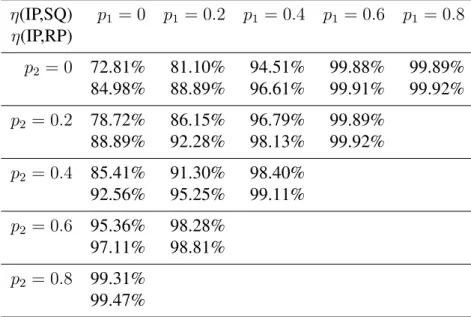
LRACIPand LRACRP−LRACSQ. Table 2.4 displays the relative efficiency of IP over SQ and Table 2.4: Relative efficiencies assuming that on average 15 patients arrive per day.

η(IP,SQ) p1 = 0 p1 = 0.2 p1 = 0.4 p1 = 0.6 p1 = 0.8 η(IP,RP)

p2 = 0 72.81% 81.10% 94.51% 99.88% 99.89% 84.98% 88.89% 96.61% 99.91% 99.92% p2 = 0.2 78.72% 86.15% 96.79% 99.89%

88.89% 92.28% 98.13% 99.92% p2 = 0.4 85.41% 91.30% 98.40%

92.56% 95.25% 99.11% p2 = 0.6 95.36% 98.28%

97.11% 98.81% p2 = 0.8 99.31%

99.47%

(52)

2.7 Extension of the Base Model: Rejection is Allowed

In this section we study an extension of the base model, where the patient’s request for an appointment can be rejected without incurring any cost except for the lost revenue.

2.7.1 Optimality Equation

Consider three cases of an arrival event when the system state is(i, j). If the arrival is of type-1, the decision is to give her an appointment on the next day or reject her, then the state changes to(i+ 1, j)or stays in(i, j), respectively. If the arrival is of type-2, the decision is to give her an appointment on the day after next or reject her, then the state changes to(i, j+ 1)

or stays in(i, j), respectively. If the arrival is of type-12, she can be assigned to the next day with state changing to(i+ 1, j), or the day after next with state changing to(i, j+ 1), or she can be rejected with state staying in(i, j).

Using the dynamics above, the optimality equation can be written as:

h(i, j) +g =α[p12min{h(i+ 1, j), h(i, j+ 1), h(i, j)}+p1min{h(i+ 1, j), h(i, j)}

+p2min{h(i, j+ 1), h(i, j)}] + (1−α)[c(i) +h(j,0)]. (2.12)

(53)

The value iteration method to solve Equation (2.12) is given by:

vk(i, j) =α[p12min{vk−1(i+ 1, j), vk−1(i, j+ 1), vk−1(i, j)}

+p1min{vk−1(i+ 1, j), vk−1(i, j)}+p2min{vk−1(i, j+ 1), vk−1(i, j)}]

+ (1−α)[c(i) +vk−1(j,0)], (2.13)

where we setv0(i, j) = 0for all(i, j)∈S.

The existence of a solution to Equation (2.12) and the convergence of the value iteration algorithm follows along similar lines as in Theorem 5. We writedt(i, j) = 1if the decision is to assign the patient to dayn+ 1,dt(i, j) = 2if the decision is to assign the patient to day

n+ 2, anddt(i, j) = 3if the decision is reject the patient. The optimal decisions are given as

below.

• For a type-1 patient,

d1(i, j) =

        

1, ifh(i+ 1, j)≤h(i, j);

3, ifh(i+ 1, j)> h(i, j).

(2.14)

d2(i, j) =

        

2, ifh(i, j+ 1)≤h(i, j);

3, ifh(i, j+ 1)> h(i, j).

(54)

d12(i, j) =

                  

1, ifh(i+ 1, j)≤min{h(i, j+ 1), h(i, j)};

2, ifh(i, j+ 1)≤min{h(i+ 1, j), h(i, j)};

3, ifh(i, j)≤min{h(i+ 1, j), h(i, j+ 1)}.

(2.16)

2.7.2 Structural Properties

In this section, we study the structural properties of the optimal policy. We start with a fundamental assumption.

Assumption A.The functionc(·)is convex and achieves its minimum at a positive integer m.

Using the parametermwe partition the state spaceS ={(i, j) : i ≥0, j ≥0}into four regions: S0, S1, S2, S3, as shown in Figure 2.3. In mathematical terms, the four regions are defined as follows:

S0 ={(i, j):0≤i≤m−1,0≤j ≤m−1}; S1 ={(i, j):0≤i≤m−1, j ≥m};

(55)

Number of scheduled appointments on day n+ 1, i 0 m N u m b er o f sc h ed u le d a p p o in tm en ts o n d a y n + 2 , j 0 m

R

0

R

1

R

2

R

3 Regions

(56)

Next we study the properties of the biash(·,·). Consider a functionf :S → _Rwith the properties

Inc(1)inS2∪S3: f(i+ 1, j)≥f(i, j), ∀(i, j)∈S2∪S3; Dec(1)inS0∪S1: f(i+ 1, j)≤f(i, j), ∀(i, j)∈S0∪S1; Inc(2)inS1∪S3: f(i, j+ 1)≥f(i, j), ∀(i, j)∈S1∪S3; Dec(2)inS0∪S2: f(i, j+ 1)≤f(i, j), ∀(i, j)∈S0∪S2;

and

ConvexityinS0:



   

   

f(i, j) +f(i+ 2, j)≥2f(i+ 1, j), ∀(i+ 1, j)∈S0;

f(i, j) +f(i, j+ 2) ≥2f(i, j+ 1), ∀(i, j+ 1)∈S0;

SuperinS0: f(i, j) +f(i+ 1, j+ 1) ≥f(i+ 1, j) +f(i, j + 1), ∀(i, j)∈S0;

andSuperC inS0:



   

   

f(i+ 2, j) +f(i, j+ 1)≥f(i+ 1, j) +f(i+ 1, j+ 1), ∀(i+ 1, j)∈S0;

(57)

We now redefine some operators as below.

T12f(i, j) = min{f(i+ 1, j), f(i, j+ 1), f(i, j)}, T1f(i, j) = min{f(i+ 1, j), f(i, j)},

T2f(i, j) = min{f(i, j+ 1), f(i, j)}.

Thenvkin Equation (2.13) can be rewritten as:

vk+1(i, j) =Tα(Tp(T12vk, T1vk, T2vk), Tcvk)(i, j),

withv0(i, j) = 0for all(i, j)∈S. The operatorsTp, Tα, Tcare defined in Section 2.4.

The following lemmas show the relevant properties of the operators.

Lemma 3. The operatorT12satisfies:

(a)Inc(1)inS2 ∪S3 →Inc(1)inS2∪S3

(b)Inc(1)inS2∪S3, Dec(1)inS0∪S1, Inc(2)inS1∪S3, Dec(2)inS0∪S2 →Dec(1)in S0∪S1

(c)Inc(2)inS1 ∪S3 →Inc(2)inS1∪S3

(d)Inc(1)inS2∪S3, Dec(1)inS0∪S1, Inc(2)inS1∪S3, Dec(2)inS0∪S2 →Dec(2)in S0∪S2

(58)

Super,SuperCinS0 →SuperinS0

(g)Inc(1)inS2∪S3, Dec(1)inS0∪S1, Inc(2)inS1∪S3, Dec(2)inS0∪S2,Convexity, Super,SuperCinS0 →SuperCinS0.

Proof. (a). The result follows since the monotonicity is closed under the minimum operator. (b). We need to showT12f(i+ 1, j) ≤ T12f(i, j)for0 ≤ i ≤ m−1, j ≥ 0. We consider three cases:

Case (b)(1):0≤i≤m−2, j ≥0. The result follows since the monotonicity is closed under the minimum operator.

Case (b)(2):i=m−1,0≤j ≤m−1. We need to showT12f(m, j)≤T12f(m−1, j). We have

Dec(2)inS0∪S2 ⇒f(m, j + 1)≤f(m, j); Inc(1)inS2∪S3 ⇒f(m, j)≤f(m+ 1, j).

Hence

T12f(m, j) = min{f(m+ 1, j), f(m, j+ 1), f(m, j)}=f(m, j + 1).

Similary, we have

Dec(1)inS0∪S1 ⇒f(m, j)≤f(m−1, j);

(59)

Hence

T12f(m−1, j) = min{f(m, j), f(m−1, j+ 1), f(m−1, j)}

= min{f(m, j), f(m−1, j+ 1)}.

We knowf(m, j + 1) ≤f(m, j)byDec(2)inS0∪S2andf(m, j + 1) ≤f(m−1, j+ 1) byDec(1)inS0∪S1. Therefore

T12f(m, j) = f(m, j + 1)≤min{f(m, j), f(m−1, j+ 1)}=T12f(m−1, j).

Case (b)(3):i=m−1, j ≥m. We need to showT12f(m, j)≤T12f(m−1, j). We have

Inc(1)inS2 ∪S3 ⇒f(m, j)≤f(m+ 1, j); Inc(2)inS1 ∪S3 ⇒f(m, j)≤f(m, j + 1).

Hence

T12f(m, j) = min{f(m+ 1, j), f(m, j + 1), f(m, j)}=f(m, j).

We have

(60)

Therefore

T12f(m−1, j) = min{f(m, j), f(m−1, j+ 1), f(m−1, j)}=f(m, j).

The result follows.

(c). The result follows since the monotonicity is closed under the minimum operator.

(d). We need to showT12f(i, j+ 1) ≤ T12f(i, j)fori ≥ 0,0 ≤ j ≤ m−1. We consider three cases:

Case (d)(1):i≥0,0≤j ≤m−2. The result follows since the monotonicity is closed under the minimum operator.

Case (d)(2):0≤i≤m−1, j =m−1. We need to showT12f(i, m)≤T12f(i, m−1). We have

Dec(1)inS0∪S1 ⇒f(i+ 1, m)≤f(i, m); Inc(2)inS1∪S3 ⇒f(i, m)≤f(i, m+ 1).

Hence

(61)

Similarly, we have

Dec(1)inS0∪S1 ⇒f(i+ 1, m−1)≤f(i, m−1); Dec(2)inS0∪S2 ⇒f(i, m)≤f(i, m−1).

Therefore

T12f(i, m−1) = min{f(i+ 1, m−1), f(i, m), f(i, m−1)}

= min{f(i+ 1, m−1), f(i, m)}

We knowf(i+ 1, m)≤f(i+ 1, m−1)byDec(2)inS0∪S2andf(i+ 1, m)≤f(i, m)by Dec(1)inS0∪S1.

T12f(i, m) =f(i+ 1, m)≤min{f(i+ 1, m−1), f(i, m)}=T12f(i, m−1).

Case (d)(3):i≥m, j =m−1. We need to showT12f(i, m)≤T12f(i, m−1). We have

Inc(1)inS2∪S3 ⇒f(i, m)≤f(i+ 1, m); Inc(2)inS1∪S3 ⇒f(i, m)≤f(i, m+ 1).

(62)

Similarly, we have

Dec(2)inS0∪S2 ⇒f(i, m)≤f(i, m−1);

Inc(1)inS2∪S3 ⇒f(i, m−1)≤f(i+ 1, m−1).

Therefore

T12f(i, m−1) = min{f(i+ 1, m−1), f(i, m), f(i, m−1)}=f(i, m).

The result follows.

(e). We show that T12f(i, j) +T12f(i+ 2, j) ≥ 2T12f(i+ 1, j)for 0 ≤ i ≤ m−2,0 ≤ j ≤m−1and skip the proof thatT12f(i, j) +T12f(i, j+ 2) ≥2T12f(i, j + 1)for0≤i≤ m−1,0≤j ≤m−2since it is similar. We consider four cases:

Case (e)(1)i≤m−3, j ≤m−1. We know

T12f(i, j) = min{f(i+ 1, j), f(i, j+ 1), f(i, j)}= min{f(i+ 1, j), f(i, j+ 1)}.

TheT12here coincides with theTR(I)in (Koole, 1998). The result follows. Case (e)(2)i≤m−3, j =m. We show

(63)

where we know

T12f(i, m) = f(i+ 1, m); T12f(i+ 2, m) = f(i+ 3, m); T12f(i+ 1, m) = f(i+ 2, m).

The result follows from theConvexityoff. Case (e)(3)i=m−2, j ≤m−1. We show

T12f(m−2, j) +T12f(m, j)≥2T12f(m−1, j),

where we know

T12f(m−2, j) = min{f(m−1, j), f(m−2, j+ 1)}; T12f(m−1, j) = min{f(m, j), f(m−1, j+ 1)};

T12f(m, j) = f(m, j + 1).

We consider two cases:

Case (e)(3)(i):f(m−1, j)≥f(m−2, j+ 1). ThenT12f(m−2, j) =f(m−2, j+ 1). By the propertySuperC off, we know

(64)

HenceT12f(m−1, j) = f(m−1, j+ 1). By theConvexity off, we have

T12f(m−2, j) +T12f(m, j) =f(m−2, j + 1) +f(m, j+ 1) ≥2f(m−1, j+ 1) = 2T12f(m−1, j).

Case (e)(3)(ii):f(m−1, j)< f(m−2, j+ 1). ThenT12f(m−2, j) = f(m−1, j). By the Superoff, we have

T12f(m−2, j) +T12f(m, j) =f(m−1, j) +f(m, j+ 1) ≥f(m, j) +f(m−1, j+ 1)

≥2 min{f(m, j), f(m−1, j + 1)}

= 2T12f(m−1, j).

Case (e)(4)i=m−2, j =m. We show

T12f(m−2, m) +T12f(m, m)≥2T12f(m−1, m),

where we know

T12f(m−2, m) = f(m−1, m); T12f(m−1, m) = f(m, m);

(65)

The result follows fromf(m−1, m)≥f(m, m)byDec(1)inS0∪S1.

(f). We show that T12f(i, j) +T12f(i + 1, j + 1) ≥ T12f(i+ 1, j) + T12f(i, j + 1) for

0≤i, j ≤m−1. We consider four cases:

Case (f)(1)i ≤ m−2, j ≤ m −2. We know T12f(i, j) = min{f(i+ 1, j), f(i, j + 1)} coincides with theTR(I)in (Koole, 1998). The result follows.

Case (f)(2)i=m−1, j ≤m−2. We show

T12f(m−1, j) +T12f(m, j + 1)≥T12f(m, j) +T12f(m−1, j+ 1),

where we know

T12f(m−1, j) = min{f(m, j), f(m−1, j + 1)}; T12f(m, j+ 1) =f(m, j+ 2);

T12f(m, j) =f(m, j+ 1);

T12f(m−1, j+ 1) = min{f(m, j+ 1), f(m−1, j+ 2)}.

(66)

Superoff, we know

T12f(m−1, j) +T12f(m, j+ 1) =f(m−1, j+ 1) +f(m, j+ 2)

≥f(m, j+ 1) +f(m−1, j+ 2)(bySuper)

≥f(m, j+ 1) + min{f(m, j+ 1), f(m−1, j+ 2)}

=T12f(m, j) +T12f(m−1, j + 1).

Case (f)(2)(ii):f(m, j)< f(m−1, j+ 1). ThenT12f(m−1, j) =f(m, j). By theSuperC off, we know

f(m, j+ 1)−f(m−1, j+ 2)≤f(m, j)−f(m−1, j+ 1)<0.

HenceT12f(m−1, j+ 1) =f(m, j+ 1). By theConvexityoff, we have

T12f(m−1, j) +T12f(m, j+ 1) =f(m, j) +f(m, j + 2) ≥f(m, j+ 1) +f(m, j+ 1)

=T12f(m, j) +T12f(m−1, j+ 1).

Case (f)(3)i≤m−2, j =m−1. We show

(67)

where we know

T12f(i, m−1) = min{f(i+ 1, m−1), f(i, m)}; T12f(i+ 1, m) =f(i+ 2, m);

T12f(i+ 1, m−1) = min{f(i+ 2, m−1), f(i+ 1, m)}; T12f(i, m) =f(i+ 1, m).

We know

T12f(i, m−1) +T12f(i+ 1, m)

= min{f(i+ 1, m−1), f(i, m)}+f(i+ 2, m)

= min{f(i+ 1, m−1) +f(i+ 2, m), f(i, m) +f(i+ 2, m)}

≥min{f(i+ 1, m−1) +f(i+ 2, m),2f(i+ 1, m)}(byConvexity)

≥min{f(i+ 2, m−1) +f(i+ 1, m),2f(i+ 1, m)}(bySuper) = min{f(i+ 2, m−1), f(i+ 1, m)}+f(i+ 1, m)

=T12f(i+ 1, m−1) +T12f(i, m).

Case (f)(4)i=m−1, j =m−1. We show

(68)

where we know

T12f(m−1, m−1) = min{f(m, m−1), f(m−1, m)}; T12f(m, m) = f(m, m);

T12f(m, m−1) =f(m, m); T12f(m−1, m) = f(m, m).

We know

T12f(m−1, m−1) +T12f(m, m) = min{f(m, m−1), f(m−1, m)}+f(m, m) ≥f(m, m) +f(m, m)(byDec(1)andDec(2)) =T12f(m, m−1) +T12f(m−1, m).

(g). We show thatT12f(i+ 2, j) +T12f(i, j+ 1) ≥T12f(i+ 1, j) +T12f(i+ 1, j+ 1)for

0 ≤ i ≤ m −2,0 ≤ j ≤ m−1. We skip the proof of T12f(i+ 1, j) +T12f(i, j + 2) ≥ T12f(i, j+ 1) +T12f(i+ 1, j + 1)for0 ≤ i ≤ m−1,0 ≤ j ≤ m−2. We consider four cases:

Case (g)(1) i ≤ m −3, j ≤ m−2. We know T12f(i, j) = min{f(i+ 1, j), f(i, j + 1)} coincides with theTR(I)in (Koole, 1998). The result follows.

Case (g)(2)i=m−2, j ≤m−2. We show

(69)

where we know

T12f(m, j) = f(m, j + 1);

T12f(m−2, j+ 1) = min{f(m−1, j + 1), f(m−2, j+ 2)}; T12f(m−1, j) = min{f(m, j), f(m−1, j+ 1)};

T12f(m−1, j+ 1) = min{f(m, j + 1), f(m−1, j + 2)}.

Case (g)(2)(i):f(m−1, j+1)< f(m−2, j+2). ThenT12f(m−2, j+1) = f(m−1, j+1). We have

T12f(m, j) +T12f(m−2, j+ 1)

=f(m, j+ 1) +f(m−1, j+ 1)

≥min{f(m, j+ 1), f(m−1, j+ 2)}+ min{f(m, j), f(m−1, j+ 1)}

=T12f(m−1, j+ 1) +T12f(m−1, j).

Case (g)(2)(ii):f(m−1, j+1) ≥f(m−2, j+2). ThenT12f(m−2, j+1) =f(m−2, j+2). We have

SuperC ⇒f(m, j+ 1)−f(m−1, j+ 2)≥f(m−1, j+ 1)−f(m−2, j + 2)≥0

(70)

and

SuperC ⇒f(m, j)−f(m−1, j+ 1)≥f(m, j+ 1)−f(m−1, j+ 2)≥0

⇒T12f(m−1, j) = f(m−1, j+ 1).

We have

T12f(m, j) +T12f(m−2, j+ 1)

=f(m, j+ 1) +f(m−2, j+ 2)

≥f(m−1, j+ 2) +f(m−1, j+ 1)(bySuperC) =T12f(m−1, j+ 1) +T12f(m−1, j).

Case (g)(3)i≤m−3, j =m−1. We show

T12f(i+ 2, m−1) +T12f(i, m)≥T12f(i+ 1, m−1) +T12f(i+ 1, m),

where we know

T12f(i+ 2, m−1) = min{f(i+ 3, m−1), f(i+ 2, m)};

T12f(i, m) =f(i+ 1, m);

(71)

Case (g)(3)(i):f(i+ 3, m−1)< f(i+ 2, m). ThenT12f(i+ 2, m−1) = f(i+ 3, m−1). We have

SuperC ⇒f(i+ 2, m−1)−f(i+ 1, m)≤f(i+ 3, m−1)−f(i+ 2, m)<0

⇒T12f(i+ 1, m−1) =f(i+ 2, m−1).

Hence

T12f(i+ 2, m−1) +T12f(i, m)

=f(i+ 3, m−1) +f(i+ 1, m)

≥f(i+ 2, m−1) +f(i+ 2, m)(bySuperC) =T12f(i+ 1, m−1) +T12f(i+ 1, m).

Case (g)(3)(ii):f(i+ 3, m−1)≥f(i+ 2, m). ThenT12f(i+ 2, m−1) = f(i+ 2, m). We have

T12f(i+ 2, m−1) +T12f(i, m) =f(i+ 2, m) +f(i+ 1, m)

≥f(i+ 2, m) + min{f(i+ 2, m−1), f(i+ 1, m)}

(72)

Case (g)(4)i=m−2, j =m−1. We show

T12f(m, m−1) +T12f(m−2, m)≥T12f(m−1, m−1) +T12f(m−1, m),

where we know

T12f(m, m−1) =f(m, m);

T12f(m−2, m) = f(m−1, m);

T12f(m−1, m−1) = min{f(m, m−1), f(m−1, m)}; T12f(m−1, m) = f(m, m).

Hence

T12f(m, m−1) +T12f(m−2, m)

=f(m, m) +f(m−1, m)

≥f(m, m) + min{f(m, m−1), f(m−1, m)}

=T12f(m−1, m) +T12f(m−1, m−1).

Lemma 4. The operatorsT1, T2satisfy (a) to (g) in Lemma 3.

(73)

oper-atorT2. Given the propertiesf has, we know

T1f(i, j) = min{f(i+ 1, j), f(i, j)}= 

   

   

f(i+ 1, j), ∀(i, j)∈S0∪S1,

f(i, j), ∀(i, j)∈S2∪S3.

We prove (f) and skip the rest due to the similarity. We show thatT1f(i, j)+T1f(i+1, j+1)≥ T1f(i+ 1, j) +T1f(i, j+ 1)for any0≤i, j ≤m−1. We consider four cases:

Case (f)(1):0≤i≤m−2,0≤j ≤m−2. We have

T1f(i, j) +T1f(i+ 1, j+ 1) =f(i+ 1, j) +f(i+ 2, j+ 1)

≥f(i+ 2, j) +f(i+ 1, j + 1)(bySuper) =T1f(i+ 1, j) +T1f(i, j + 1).

Case (f)(2):i=m−1,0≤j ≤m−2. We need to showT1f(m−1, j) +T1f(m, j+ 1)≥ T1f(m, j) +T1f(m−1, j+ 1). We have

T1f(m−1, j) +T1f(m, j+ 1) =f(m, j) +f(m, j + 1)

=T1f(m, j) +T1f(m−1, j+ 1)

(74)

T1f(i+ 1, m−1) +T1f(i, m). We have

T1f(i, m−1) +T1f(i+ 1, m) = f(i+ 1, m−1) +f(i+ 2, m)

≥f(i+ 2, m−1) +f(i+ 1, m)(bySuper) =T1f(i+ 1, m−1) +T1f(i, m).

Case (f)(4): i =m−1, j =m−1. We need to showT1f(m−1, m−1) +T1f(m, m)≥ T1f(m, m−1) +T1f(m−1, m). This follows because

T1f(m−1, m−1) +T1f(m, m) =f(m, m−1) +f(m, m)

=T1f(m, m−1) +T1f(m−1, m).

Lemma 5. The operatorsTp, Tαsatisfy: (a)Inc(1)inS2 ∪S3 →Inc(1)inS2∪S3

(b)Dec(1)inS0∪S1 →Dec(1)inS0∪S1

(d)Dec(2)inS0∪S2 →Dec(2)inS0∪S2

(e)ConvexityinS0 →ConvexityinS0

(f)SuperinS0 →SuperinS0

(75)

Proof. Given the definition ofTpandTα, the conditions (a) to (g) follow, since the properties

are closed under convex combination.

Lemma 6. Under the AssumptionA. The operatorTcsatisfies: (a)Inc(1)inS2 ∪S3 →Inc(1)inS2∪S3

(b)Dec(1)inS0∪S1 →Dec(1)inS0∪S1

(d)Dec(1)inS0∪S1 →Dec(2)inS0∪S2

(e)Convexity, Super, SuperC inS0 →ConvexityinS0

(f)Convexity, Super, SuperC inS0 →SuperinS0

(g)Convexity, Super, SuperC inS0 →SuperC inS0.

Proof. We know Tcf(i, j) = c(i) +f(j,0)and c(x) is a convex function which achieves

its minimum at x = m, hence (a) and (b) follow. For (c), if f is Inc(1)inS2 ∪ S3, then f(i+ 1, j) ≥ f(i, j),∀i ≥ m, j ≥ 0. For any j ≥ m, we have Tcf(i, j + 1) = c(i) +

f(j + 1,0) ≥ c(i) +f(j,0) = Tcf(i, j). HenceTcf isInc(2)inS1 ∪S3. For (d), iff is Dec(1)inS0 ∪S1, then f(i+ 1, j) ≤ f(i, j),∀i ≤ m −1, j ≥ 0. For any j ≤ m −1, we have Tcf(i, j + 1) = c(i) +f(j + 1,0) ≤ c(i) +f(j,0) = Tcf(i, j). Hence Tcf is

(76)

is trivially shown given the definition of the operatorTc. For (g), we have

≥c(i+ 1) +f(j,0) +c(i+ 1) +f(j + 1,0)

=Tcf(i+ 1, j) +Tcf(i+ 1, j+ 1),

and

≥c(i) +f(j + 1,0) +c(i+ 1) +f(j+ 1,0)

=Tcf(i, j+ 1) +Tcf(i+ 1, j+ 1).

Next we prove the properties of the biash(·,·).

Theorem 10. Under Assumption A, the bias h(·,·) satisfies properties Inc(1) in S2 ∪S3, Dec(1)inS0∪S1,Inc(2) inS1∪S3, Dec(2) inS0 ∪S2 andConvexity,Super,SuperC

inS0.

Proof. By the lemmas above, the induction hypothesis gives rise to the fact that the functions vksatisfy these properties. By Theorems 4 and 5, the biash(·,·)has these properties.

(77)

Corollary 2. The optimal decisions are given as follows.

• For a type-1 patient, we have

d1(i, j) =

        

1, ifi≤m−1.

3, ifi≥m.

d2(i, j) =

        

2, ifj ≤m−1.

3, ifj ≥m.

d12(i, j) =

        

d, if(i, j)∈Sd, whered= 1,2,3.

1or2, if(i, j)∈S0.

and for(i, j)∈S0,

d12(i, j) = 1⇒d12(i, j+ 1) = 1, d12(i, j) = 2 ⇒d12(i+ 1, j) = 2.

Proof. Follows directly from Theorem 10 and equations (2.14) to (2.16).

(78)

Theorem 11. Under Assumption A, for 0 ≤ i ≤ m − 1, there exists a critical number

j∗(i)≤mand for0≤j ≤m−1there exists a critical numberi∗(j)≤msuch that

d12(i, j) =                   

1, ifi≤m−1, j ≥j∗(i)

2, ifi≥i∗(j), j ≤m−1

3, ifi≥m, j ≥m.

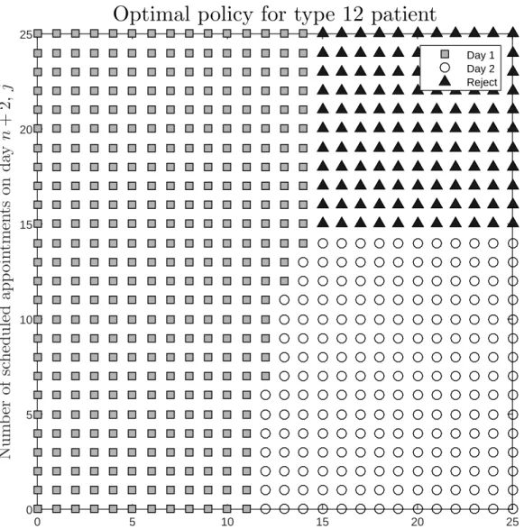
2.7.3 Numerical Illustration

We now conduct a numerical study to illustrate the structural properties of the optimal policy. We use the same parameters as in Section 2.4.1. The only difference is that rejection is available here. Figure 2.4 displays the optimal decision for a type-12 patient in each state. We do not display the optimal decisions for type-1 or type-2 patient because the policy is explicitly given by Corollary 2. Figure 2.4 indicates that it is optimal to stop scheduling a patient on any day once the number of scheduled appointments on that day reachesm.

2.7.4 Heuristic Policies

(79)

Number of scheduled appointments on day n+ 1, i

0 5 10 15 20 25

N u m b er o f sc h ed u le d a p p o in tm en ts o n d a y n + 2 , j 0 5 10 15 20 25