STOCHASTIC MODELS FOR RESOURCE ALLOCATION, SERIES PATIENTS SCHEDULING, AND INVESTMENT DECISIONS
Siyun Yu
A dissertation submitted to the faculty of the University of North Carolina at Chapel Hill in partial fulfillment of the requirements for the degree of Doctor of Philosophy in the
Department of Statistics and Operations Research.
Chapel Hill 2017
Approved by:
Vidyadhar G. Kulkarni Nilay Argon
Vinayak Deshpande Nur Sunar
c
O2017 Siyun Yu
ABSTRACT
SIYUN YU: STOCHASTIC MODELS FOR RESOURCE ALLOCATION, SERIES PATIENTS SCHEDULING, AND INVESTMENT DECISIONS
(Under the direction of Vidyadhar G. Kulkarni.)
We develop stochastic models to devise optimal or near-optimal policies in three different areas: resource allocation in virtual compute labs (VCL), appointment scheduling in healthcare facilities with series patients, and capacity management for competitive investment.
A VCL consists of a large number of computers (servers), users arrive and are given access to severs with user-specified applications loaded onto them. The main challenge is to decide how many servers to keep “on”, how many of them to preload with specific applications (so users needing these applications get immediate access), and how many to be left flexible so that they can be loaded with any application on demand, thus providing delayed access. We propose dynamic policies that minimize costs subject to service performance constraints and validate them using simulations with real data from the VCL at NC State.
In the second application, we focus on healthcare facilities such as physical therapy (PT) clinics, where patients are scheduled for a series of appointments. We use Markov Decision Processes to develop the optimal policies that minimize staffing, overtime, overbooking and delay costs, and develop heuristic secluding policies using the policy improvement algorithm. We use the data from a local PT center to test the effectiveness of our proposed policies and compare their performance with other benchmark policies.
ACKNOWLEDGEMENTS
I would like to gratefully acknowledge the guidance, support and encouragement of my doctoral advisor, Dr. Kulkarni. I have been extremely lucky to have a supervisor who cared so much about my work, and who responded to my questions and queries so promptly. I would also like to thank all the members of my committee during my time at UNC STOR Department, for their input, valuable discussions and accessibility
My gratitude extends to Dr. Deshpande and Dr. Sunar of UNC Kenan-Flagler Business School, and Dr. Shen of HKU, for their enthusiasm, advice and support in the three projects. Without their expertise, I would not have been able to continue and complete the three projects presented in this dissertation.
TABLE OF CONTENTS
LIST OF FIGURES . . . x
LIST OF TABLES . . . xii
CHAPTER 1: Introduction . . . 1
1.1 Application 1. Server Configuration in Cloud Computing. . . 1
1.2 Application 2. Appointment Systems for Series Patients . . . 3
1.3 Application 3. Investment Capacity and Timing Management . . . 4
CHAPTER 2: Statistical Forecasting and Queueing Models for Virtual Com-puting Labs . . . 6
2.1 Introduction . . . 6
2.2 Literature Review . . . 9
2.3 Data . . . 12
2.3.1 Arrivals . . . 13
2.3.2 Service Times . . . 14
2.4 Queueing Models and Staffing Policies . . . 15
2.4.1 Problem Formulation - Static SAP . . . 15
2.4.2 Queueing Models for Static SAP . . . 16
2.4.3 Dynamic SAP . . . 24
2.5 Forecasting Future Arrival Demand . . . 26
2.5.1 Moving Average Forecasting . . . 27
2.5.2 SVD Forecasting . . . 27
2.6.1 M/G/c/c Queue. . . 31
2.6.2 MX/M/∞ Queue. . . 32
2.6.3 M(t)/G/∞ Queue. . . 33
2.7 Recommendations . . . 33
2.8 Summary and Extensions . . . 34
CHAPTER 3: Staffing and Scheduling for Health Care Facilities with Series Patients: Model I . . . 38
3.1 Introduction . . . 38
3.2 Literature Review . . . 41
3.3 The Model . . . 42
3.4 The Optimal Staffing Policy . . . 46
3.5 Optimal Scheduling Policies . . . 48
3.5.1 Structural Properties of the Optimal Policy . . . 51
3.6 Implementable Policies . . . 54
3.6.1 Randomized policy (RP) . . . 54
3.6.2 Shortest Queue (SQ) policy . . . 56
3.6.3 Max-Marginal Profit (MP) policy . . . 57
3.6.4 Policy Improvement Heuristics: Index policy . . . 58
3.6.5 Policy Improvement Heuristics: Min-Cost Flow (MF) policy . . . 63
3.6.6 Structural Properties of the Implementable Policies . . . 63
3.7 Numerical Examples with Real Data . . . 65
3.8 Conclusions and Extensions . . . 69
CHAPTER 4: Staffing and Scheduling for Health Care Facilities with Series Patients: Model II . . . 71
4.1 Introduction . . . 71
4.2 The Model II . . . 71
4.3.1 Special Case: Geometric Number of Visits . . . 76
4.4 Implementable Policies . . . 77
4.4.1 Next Day Policy (NDP) . . . 77
4.4.2 Shortest Queue Policy (SQP) . . . 79
4.4.3 Index Policy (IP) . . . 79
4.4.4 Index Policy with Geometric Assumption (GIP) . . . 84
4.5 Numerical Examples with Real Data . . . 85
4.5.1 Comparison of Policies . . . 86
4.5.2 Optimal Staffing . . . 88
4.5.3 Value of Modeling Series Patients . . . 88
4.6 Conclusions and Extensions . . . 90
CHAPTER 5: Optimal policies for Investment Capacity and Timing . . . 91
5.1 Introduction . . . 91
5.1.1 Summary of Main Results . . . 93
5.1.2 Literature Review . . . 94
5.2 The Model . . . 97
5.3 Analysis . . . 100
5.3.1 Follower’s Problem . . . 100
5.3.2 Leader’s Problem and Equilibrium Strategies . . . 103
5.4 Numerical Experiments . . . 110
5.5 Minimum Capacity Investment Requirement . . . 111
5.6 Summary . . . 117
APPENDIX A:APPENDICES . . . 119
A.1 Appendices for Chapter 2 . . . 119
A.1.1 Additional Plots for Sample Applications . . . 119
A.1.3 A3. NHPP Tests on the Arrival Data . . . 121
A.1.4 Additional Simulation Results . . . 122
A.2 Appendices for Chapter 3 . . . 122
A.2.1 Proof of Theorem 3.1 . . . 122
A.2.2 Proof of Theorem 3.2 . . . 123
A.2.3 Proof of Theorem 3.3 . . . 123
A.2.4 Proof of Theorem 3.4 . . . 124
A.2.5 Proof of Theorem 3.5 . . . 126
A.2.6 Proof of Theorem 3.6 . . . 126
A.2.7 Proof of Corollary 3.1 . . . 127
A.2.8 Proof of Corollary 3.2 . . . 127
A.2.9 Proof of Proposition 3.1 . . . 128
A.2.10 Proof of Proposition 3.2 . . . 128
A.2.11 Solution to Min-Cost Flow Problem . . . 129
A.2.12 Proof of Theorem 3.7 . . . 130
A.3 Appendices for Chapter 5 . . . 132
A.3.1 The Heuristic Derivation of the HJB Equation (5.10) . . . 132
A.3.2 Proof of Proposition 5.1 . . . 133
A.3.3 Proof of Proposition 5.2 . . . 140
A.3.4 Proof of Proposition 5.3 . . . 141
A.3.5 Proof of the Main Result . . . 144
A.3.6 The Heuristic Derivation and the Solution of (5.21) . . . 156
A.3.7 Proof of Proposition 5.4 . . . 157
A.3.8 Proof of Proposition 5.5 . . . 160
A.3.9 Proof of Proposition 5.6 . . . 163
A.3.10 Proof of Proposition 5.7 . . . 170
A.3.12 Proof of Proposition 5.9 . . . 173 A.3.13 Proof of Proposition 5.11. . . 176
LIST OF FIGURES
2.1 VCL Servers Network Diagram . . . 8
2.2 Aggregated Arrivals . . . 13
2.3 Arrivals of Application 1 . . . 13
2.4 Mean and Standard Deviation of Aggregated Arrivals by Day of Week . . . 14
2.5 Empirical CDF of Service Times and Exponential CDF . . . 15
2.6 Scree Plots . . . 29
2.7 Simulation Results of M/G/c/c Queue . . . 36
2.8 Comparison of Three Queueing Models . . . 37
3.1 Daily Net Profit as Function ofD . . . 47
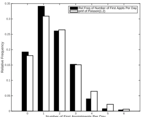
3.2 Distribution of Number of Daily (First) Appointments . . . 66
3.3 Distribution of Total Number of Appointments Per Patient . . . 66
3.4 Average Profits under Index Policy as a Function of q in Case A withλ= 6. . . . 69
3.5 Average Profits under Index Policy as a Function of q in Case B with λ= 6 . . . . 69
4.1 Daily Net Profit as Function ofD . . . 72
4.2 Case A, λ= 1.2 . . . 89
4.3 Case A, λ= 6 . . . 89
4.4 Case B, λ= 1.2 . . . 89
4.5 Case B, λ= 6 . . . 89
5.1 Feasible Regions for H0 and H1 . . . 107
5.2 V1 as Functions of y0, and LST ofτ as Function ofK1 . . . 109
5.3 Leader’s equilibrium capacity K1e as functions ofy0 by different values of µ1,H . . . 110
5.4 V1 as Functions of y0, and LST ofτ as Function ofK1 . . . 115
A.1 Arrivals of Application 10 . . . 119
A.3 Simulation Results ofMX/M/∞ Queue . . . 187
A.4 Simulation Results ofM(t)/G/∞ Queue . . . 188
A.5 Network Model of Optimization Problem . . . 189
A.6 f`(y) exploding with `= 0.01 . . . 189
LIST OF TABLES
2.1 Cumulative Relative Frequency of Arrivals . . . 12
3.1 Daily Average Profits and Differences from MF Policy in Case A . . . 67
3.2 Daily Average Profits and Differences from MF Policy in Case B . . . 67
4.1 Average Profits and Improvement from NDP in Case A . . . 87
4.2 Average Profits and Improvement from NDP in Case B . . . 87
CHAPTER 1: Introduction
Stochastic models are extensively used in devising resource allocation policies in many fields, such as call centers, healthcare systems, cloud computing, production systems, etc. Resource allocation plays a critical role in balancing the demand and supply, with the goal of optimizing the economical or social benefits.
Discrete and continuous stochastic models provide appropriate tools to quantify the per-formance of policies in these applications, including service quality, management profit and cost, etc. Queueing models are useful in service systems where queues arise from the mismatch of supply and demand. They can be used to obtain implementable policies to manage these systems. Continuous models such as Brownian models are useful in describing the uncertain behaviour of system evolution in response to control policies, and can be used in devising optimal control policies to manage such systems.
In this dissertation we use both discrete and continuous stochastic models to allocate re-sources in three different applications. In the rest of this chapter, we introduce the background and motivation for each one of them.
1.1 Application 1. Server Configuration in Cloud Computing.
A cloud computing system provides computing service (such as sharing data and processing resources) through internet to clients. It allows companies to decrease the IT related infras-tructure and management costs, at the same time get access to storage or a flexible collection of software applications through a simple web-based interface. In such systems, the service providers are computer servers, while the customers are the clients who generate requests of accessing the computing resources. The clients may belong to different classes and their arrival rates may vary with time. The configuration of the computer capacity allocated to the client for a given type of computing service can be controlled to guarantee the service quality.
Computing Lab (VCL). Such a system provides users remote access to their desired set of software applications. There are usually hundreds or even thousands of software applications that the users may choose from. Some examples of application are “Matlab on Windows 7”, “Maple on Windows XP”, and “Arena and CPLEX OPL” etc. Currently UNC-Chapel Hill and NC State both host hundreds of computer servers for students, faculty, and researchers. Each user is granted full control of the assigned server. If two users request the same software application, they will need two different servers loaded with that application.
The servers in the VCL may be on or off. The on servers may be preloaded with specific applications, or left flexible. When a user requests a server with a specific application, and one such server preloaded with that application is available, the user request can be satisfied immediately. If such a server is not available, we can load the application on a flexible server and make it available to this user. However, this loading operation creates a delay and degrades service somewhat. Turning an off server on usually takes too long to do in response to a user request, and hence if all servers are busy, the user leaves without service, which is the worst outcome for the user. The number of on servers can be changed during the day in an exogenous fashion in response to anticipated demand.
The main issue for the VCL is to decide on how many servers should be kept on (the rest are left off to save energy). Further, we need to decide how many of the on servers should be preloaded with which applications, and how many servers should be left flexible. The service quality can be measured in terms of the fraction of the users who get immediate access, the fraction that gets delayed access, and the fraction that gets rejected.
1.2 Application 2. Appointment Systems for Series Patients
In a health care unit, the service providers are nurses, doctors, etc, while the customers are patients. The nurses and doctors can be specialized to serve multiple classes of patients. The number of nurses and doctors on duty can be controlled to satisfy the patients demands so as to provide a certain quality assurance. The patients can belong to multiple classes, and their arrival rates may vary with time; they may need multiple visits to the clinic, (as in a physical therapy (PT) setting); they may have preferences about appointment schedules, and may display no-show and cancellation behaviors.
In Chapter 3 and 4, we focus on special clinics such as physical therapy, where patients are scheduled for repeated visits at the time of admission. Such patients are called series patients. Patients in need of physical therapy are referred by the physician to the physical therapy clinic. A clinic administrator schedules a first appointment for an initial examination. Based on the diagnosis of the patient, a plan of care is determined by the physical therapist. Such a plan includes the frequency of the visits, total number of visits, and duration of each visit. Based on the plan of care, an administrator in the clinic generates an appointment schedule. The frequency, duration and length of the appointment time for the follow up visits vary greatly depending upon the patient’s diagnosis and/or specific needs as well as the referring physician’s orders.
In Chapter 3, we consider a model where the plan of care for a patient is set up at begin-ning, so once the patient is evaluated, the number of visits is known. Under this assumption, the randomness comes from the initial evaluation, after which the series of appointments are scheduled without uncertainty. In Chapter 4, we study an alternate model where the random-ness occurs after each visit of a patient. Specifically, whether a patient needs the next visit is evaluated after every appointment. These two models capture different features of the series patients, depending on whether their treatment can be predetermined or needs to be modified based on their recovery status.
Decision Process model that can be used to compute an optimal appointment schedule for each patient. Unfortunately, the large state space makes this method impractical computationally. However, this model helps us devise a simple heuristic policy, called the index policy, that can be obtained by using policy improvement algorithm. We use simulation to show that the index policy provides better performance than other benchmark policies used in practice.
1.3 Application 3. Investment Capacity and Timing Management
When companies plan to introduce a new product or a new technology to the market, the actual demand is uncertain at the very beginning. A common scenario is that, after one firm (called the leader) initiates an investment, the competitors (called the followers) start observing the performance of this leader firm and make their decisions accordingly. In particular, there are two most critical decisions for the follower firms to make, the first is the investment capacity, that is how much to invest so as to better suit the unknown market demand, the second is the investment timing, that is when to enter the market so as to make profit with enough knowledge about the market.
We are particularly interested in competitive relations between the leader and follower firms. Once the follower enters the market, it takes part of the market share from the leader, and after that the overflow from either of the firms cannot be fulfilled by the other party, even if the other party has extra supply. This is an appropriate model for products or technologies that have a high customer loyalty so that once the customers subscribe to one of the brands, the chance for them to switch brands is very small. One example is the competitive relation between Apple and Amazon. Both firms recently invested in the development of smart speakers, a smart device controlled by human voice so that the users can play music, control echo-home systems, call taxis, etc. Since the two companies use different operating systems, all the built-in applications and other supportive devices (cell phone, smart TVs) are not compatible with each other. Therefore it is costly for the customers to switch the brands.
one of the binary status: high and low. A leader enters the market at the beginning of the horizon, and a follower starts its observation of the leader’s earning process and decides on when and how much to invest. The leader, knowing that the follower will adopt the optimal investment strategy based on the leader’s action, optimizes its strategy about how much to invest at the beginning.
CHAPTER 2: Statistical Forecasting and Queueing Models for Virtual Computing Labs
2.1 Introduction
The Virtual Computing Lab (VCL) is a cloud computing service that provides users remote access to their desired set of software applications. There are usually hundreds or even thou-sands of software applications that the users may choose from. Some examples of applications are “Matlab on Windows 7”, “Maple on Windows XP”, “Matlab and MS Excel on Windows 7”, “Arena and CPLEX OPL”, etc. The VCL was first developed at North Carolina State University (NC State) and is now an open-source project at the Apache Software Foundation - http://vcl.apache.org. An increasing number of institutions are hosting VCL servers, for ex-ample, UNC-Chapel Hill and NC State currently have hundreds of such servers for students, faculty, and researchers. From the perspective of modeling, we do not distinguish between the terms - “virtual computer” and “virtual machine”, instead we use the generic term “server”. Each user is granted full control of the assigned server. If two users request the same software application, they will need two different servers loaded with that application.
A server in the VCL may be preloaded with a specific application, or left flexible. A user gets immediate access to a server preloaded with the desired application if one is available. Otherwise, the user has to wait for several minutes until a flexible server is loaded with the desired application. In this chapter we are concerned with the issue of deciding how many servers should be preloaded with which applications, and how many servers should be left flexible. We call the preloaded and flexible servers the on servers, and the rest of the servers theoff servers that are turned off for cost saving (both energy and management). The service quality is measured by the fraction of the users who get immediate access, and the fraction that get delayed access, while the system cost is measured by the number ofonservers.
applicable to software as a service (SaaS) in cloud computing. In such large-scale computing environments, the energy consumption is an important issue, both economically and environ-mentally. Hence, it is important and relevant to dynamically allocate “the right number of on servers with the right capabilities”.
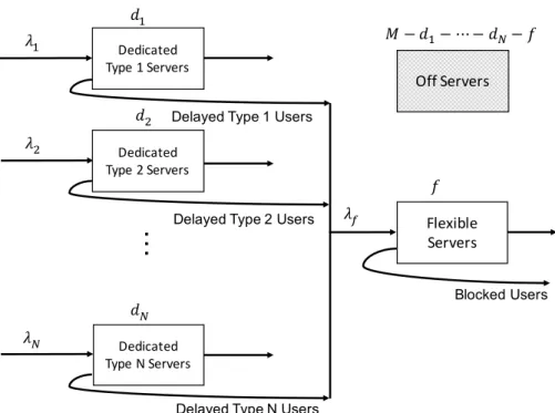
In many VCLs such as those at UNC-Chapel Hill and NC State, all servers are always on and there are no flexible servers. For example, the VCL at NC State has about 800 servers and 1600 applications; the current policy ranks the applications by the frequency with which an application is requested, and each of the 400 most popular applications are preloaded on two servers (each preloaded server has exactly one application). In general, assume the VCL has a total ofM servers and is capable of handlingN types of application. A user who desires type n(1≤n≤N) application is called a typen user. A type n user arriving at the system receives instant service if a server preloaded with application n is available. Otherwise, the user is delayed and needs to wait until the system manager (an automated software) chooses a k-preloaded server (k 6= n), removes application k and loads application n. If no server is available then this user is blocked (rejected). After a user finishes the session, the system manager wipes the server clean, and then reloads it with the same or another application.
A server allocation plan (SAP) decides how many servers should be pre-loaded with which applications, how many servers should be kept flexible, and how many should be turned off. An SAP is called dynamic if these numbers change with time; otherwise it is called static. It makes sense to consider dynamic SAPs to accommodate time-varying demand rates. Such time-varying demand is an inherent feature to the VCL system. This is caused by the seasonal demand induced by the semesters, the days of week, and the time of the day. In this chapter, we propose a dynamic SAP with the objective of minimizing the system cost while achieving the targeted service quality.
We shall begin with a static SAP assuming constant arrival rates. We keep dn servers preloaded with application n (i.e. the dedicated type n server pool, 1 ≤ n ≤ N), f servers flexible (i.e. the flexible pool), andM−f−PN
Dedicated Type N Servers
Dedicated Type 1 Servers
Flexible Servers Dedicated
Type 2 Servers
Off Servers 𝜆"
𝜆#
𝜆$
𝑑"
𝑑#
𝜆&
𝑓
𝑀 − 𝑑"− ⋯ − 𝑑$− 𝑓
𝑑$
…
Delayed Type 1 Users
Delayed Type 2 Users
Delayed Type N Users
Blocked Users
Figure 2.1: VCL Servers Network Diagram
wait a few extra minutes for the loading operation. If no flexible servers are available, the user leaves the system without service, even if there are idle servers in other dedicated pools. When a typen user finishes service from the dedicated pool, the released server is wiped clean and is reloaded with the same application to keep dn a constant. Similarly, when a user finishes service from the flexible pool, the released server is left flexible to keep f a constant.
Our proposed policy uses a dynamic SAP (see Section 2.7 for details) under which at most 10% users are delayed and at most 0.1% of the service requests are blocked. The policy only uses a maximum of 300 on servers at any time, resulting in substantial energy savings. In contrast, Lee (2013) shows that, under the current policy followed by the VCL at NC State, over 11% of the users are delayed and no users are blocked but all the available servers are always kept on. This makes our proposed policy extremely attractive.
It is clear that we need the forecasts of the arrival rates λn (1≤ n≤ N) for each period in order to execute our SAP. We explore two statistical methods to forecast the future arrival rates: the moving average (MA) method and the singular value decomposition (SVD) method. These arrival rate forecasts are then used as inputs to the queueing models to estimate the blocking probabilities. For the input parameters to the queueing models, we use either the mean arrival rate forecast or the upper bound of the 95% prediction interval of the mean arrival rate.
The remainder of the chapter is as follows. We provide a literature review on the related topics in Section 2.2. Section 2.3 introduces the structure of the data, and highlights the challenges posed by time-varying demands. We formulate our static SAP model in Section 2.4.1 and construct three static queueing models in Section 2.4.2. Algorithms are developed there to quantify the constraints in the allocation model. Section 2.4.3 explains our procedure of creating the dynamic SAP based on the static SAP introduced in Section 2.4.2. Section 2.5 introduces two ways of forecasting future arrival rates, and Section 2.6 describes how we conduct discrete event simulations using real data and presents the results. Section 2.7 makes recommendations about the most implementable policy as the combination of the best forecasting method, the estimation approach, and the queueing model. Finally, Section 2.8 summarizes the chapter and discusses how we can extend the current work to applications beyond VCL.
2.2 Literature Review
similar to our dedicated idle servers, where the user receives immediate service; their servers in setup state (switching from off to on) are similar to our flexible idle servers, where the user has to wait for some extra setup time. Two performance measurements are usually considered in a server farm setting: waiting time and power consumption. In their work, Gandhi et al. used queueing model and simulations to derive these metrics. One of their conclusions is that keeping the servers idle is superior for reducing waiting time, and turning the servers off is superior for reducing power. Adan et al. [2013] used a constant setup cost instead of a setup time to discourage switching between off and on, which simplified the state space and resulted in a switching-curve structure of the optimal policy.
Our model differs from the above server farm models in two important aspects. First, in the papers mentioned above, the users are homogeneous and the systems are stationary, while in our system, there are multiple types of users with time-varying arrival rates and service times. Second, the server farm literature deals with waiting times and power consumption, while our model focuses more on the fraction of delayed or blocking users. The use of dedicated servers is essential to reduce the fraction of delayed servers.
In this chapter we address three main features of the VCL systems: (1) time-varying de-mands, (2) multi-type demand structure, and (3) availability of data to forecast future demand. We shall review the relevant literature below in each of these areas.
The phenomenon of time-dependent arrival is commonly seen in many service systems, and it is critical to staff them at appropriate levels to cope with this variation. There is a large literature dedicated to this problem. For an in-depth review on determining the staffing levels in the presence of time-varying demand, see Green et al. [2007], Whitt [2007], Liu and Whitt [2011, 2012]; Liu et al. [2014].
when the Markovian model with sinusoidal arrival rates is considered in the simulation, the SIPP approach underestimates the staffing levels. Thompson [1993] and Green et al. [2001, 2007] have addressed this issue and discussed several solutions such as a lagged SIPP, which essentially shifts the arrival rate curve to the right by a fixed amount.
In our work, we apply approaches similar to SIPP to deal with the time-varying demand issue. Furthermore, we propose stationary dependent period by period (SDPP) approach that takes into account the customers that remain in the system from the previous period. The SDPP approach outperforms the regular SDPP approach in the service quality while using fewer servers.
The second feature is the existence of the multiple types of users. This heterogeneity in the sources of demands creates the critical issue of whether to use dedicated (specialized) or flexible resources. When the servers have sufficiently overlapping capabilities and work as a single super-server, the best possible performance can be achieved by the complete resource pooling strategy. See, for example, Harrison [1988, 2000]. Between the extremes of full-flexibility and full-specialization, different limited-flexibility structures can be constructed. Jordan and Graves [1995] are the first to show that well-designed limited flexibility can be as good as full flexibility. These principles are further justified by Akcsin and Karaesmen [2007], Iravani et al. [2007] and Bassamboo et al. [2008]. They also propose methods to evaluate different flexibility structures. Our model considers the combination of dedicated server pools and a flexible server pool, in order to provide immediate service as much as possible while guaranteeing an overall service quality.
arrival rates over intervals of 15, 30, or 60 minutes length, with a one-day lead time. More recently, Shen and Huang [2008] propose a statistical model for forecasting call volumes within short time periods of a given day and also provide approaches to account for intraday forecast updating. Their singular value decomposition (SVD) based method outperforms existing fore-casting methods. Our work adopts their SVD forefore-casting model to the VCL setting. Numerical experiments show that it leads to better service quality over the standard moving average (MA) method.
2.3 Data
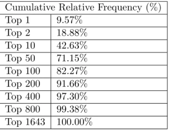
The VCL data set from NC State University contains information about all user requests from August 1, 2008 to July 31, 2011. In total there are 595,000 service requests for 1,643 different applications. For the ease of presentation, we sort the applications by their frequency of use in descending order. The usages vary considerably for different applications, where the top two applications account for 18.88%, the top ten applications account for 42.63%, and the top 400 applications account for 97.30% of the total requests. On the other hand, each of the bottom eight hundred applications is used no more than ten times over the three-year period that we consider. The detailed information is presented in Table 2.1. The VCL has around 700 to 900 servers. (The information about the exact number of servers is not given in our data set. The real time information about the number of on/off servers is given on the VCL website.) We present below some details of the arrival and service time data.
Cumulative Relative Frequency (%) Top 1 9.57%
Top 2 18.88% Top 10 42.63% Top 50 71.15% Top 100 82.27% Top 200 91.66% Top 400 97.30% Top 800 99.38% Top 1643 100.00%
2.3.1 Arrivals
Figure 2.2 (a) plots the aggregated hourly arrivals from August 1, 2008 to July 31, 2011. To provide a better idea of arrival pattern in finer time scales, we use Panels (b) and (c) to show the average hourly arrivals in each hour of the week (starting with Sunday midnight) and each hour of the day (starting with midnight) respectively. We also present the same set of graphs for individual applications as comparison. For illustration, Figure 2.3 is shown here for Application 1, while Figures A.1 and A.2 (see Appendix A.1.1) are for Applications 10 and 100.
Time Since 08/01/2008 (hr)#104 0 0.5 1 1.5 2 2.5
Number of Arrivals
0 50 100 150 200 250 (a)
Hour in Week
0 50 100 150
Average Number of Arrivals
0 5 10 15 20 25 30 35 40 45 50 (b)
Hour in Day
0 5 10 15 20
Average Number of Arrivals
0 5 10 15 20 25 30 35 40 (c)
Figure 2.2: Aggregated Arrivals
Time Since 08/01/2008 (hr)#104 0 0.5 1 1.5 2 2.5
Number of Arrivals
0 10 20 30 40 50 60 70 80 90 (a)
Hour in Week
0 50 100 150
Average Number of Arrivals
0 1 2 3 4 5 6 7 8 9 10 (b)
Hour in Day
0 5 10 15 20
Average Number of Arrivals
0 0.5 1 1.5 2 2.5 3 3.5 4 4.5 5 (c)
Figure 2.3: Arrivals of Application 1
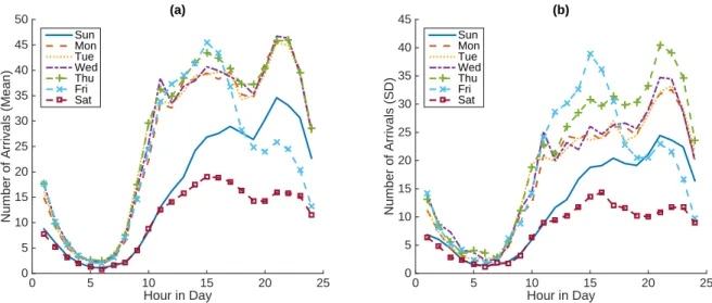
Fig-ure 2.3(b) we see that for application 1 the arrival volumes are low on Saturdays and high on Fridays. During the day, the first peak occurs around 3PM, followed by a second peak around 10PM. This is true in the aggregated case (Figure 2.3(c)) and for most of the applications. We observe that not all the applications were available in the VCL on the initial date of 08/01/2008. For example, application 10 was not available until 08/18/2010 (Figure A.1 in the appendix). Using the aggregated arrival data we also plot the mean and standard deviation against the time of day, grouped by the day of week, as shown in Figure 2.4. We observe the heteroscedas-ticity phenomenon - both the mean and the standard deviation depends on time. Besides, the magnitude of the standard deviation is almost at the same level of the mean; hence the variance exceeds the mean, which implies that the observations are over-dispersed with respect to a Poisson distribution.
Hour in Day
0 5 10 15 20 25
Number of Arrivals (Mean)
0 5 10 15 20 25 30 35 40 45
50 (a)
Sun Mon Tue Wed Thu Fri Sat
Hour in Day
0 5 10 15 20 25
Number of Arrivals (SD)
0 5 10 15 20 25 30 35 40
45 (b)
Sun Mon Tue Wed Thu Fri Sat
Figure 2.4: Mean and Standard Deviation of Aggregated Arrivals by Day of Week
2.3.2 Service Times
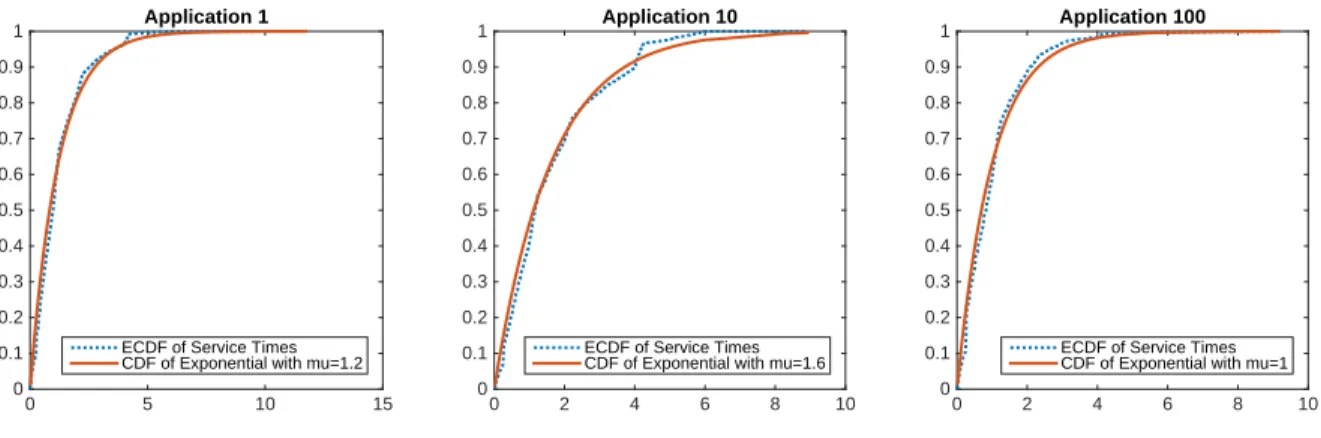
In Figure 2.5 we plot the empirical cumulative distribution function (CDF) of the service times for applications 1, 10, 100, along with the corresponding CDF of the exponential distri-bution with the same mean. The plots suggest that an exponential assumption on the service time distribution is reasonable. (Though we do not need this exponential assumption in most of our queueing models.)
0 5 10 15
0 0.1 0.2 0.3 0.4 0.5 0.6 0.7 0.8 0.9
1 Application 1
ECDF of Service Times CDF of Exponential with mu=1.2
0 2 4 6 8 10
0 0.1 0.2 0.3 0.4 0.5 0.6 0.7 0.8 0.9
1 Application 10
ECDF of Service Times CDF of Exponential with mu=1.6
0 2 4 6 8 10
0 0.1 0.2 0.3 0.4 0.5 0.6 0.7 0.8 0.9
1 Application 100
ECDF of Service Times CDF of Exponential with mu=1
Figure 2.5: Empirical CDF of Service Times and Exponential CDF
2.4 Queueing Models and Staffing Policies
As described in Section 2.1, we consider a VCL with M servers, N applications, and N
dedicated server pools (of sizes d1, d2,· · ·, dN), one flexible server pool of size f, and the rest being off servers (Figure 2.1). In this section we develop server allocation plans (SAP) for the VCL. In Section 2.4.1, we first assume that the arrival rates for the applications are constant, and present the formulation of a static SAP. Then in Section 2.4.2, we consider three queueing models for the VCL system and derive the corresponding static SAP. In Section 2.4.3, we extend the static SAP to dynamic SAP using stationary independent period by period (SIPP) and a modification version that allows dependence between periods of (SDPP).
2.4.1 Problem Formulation - Static SAP
Under the static SAP, we are interested in policies which assign dn dedicated servers preloaded with application n (1 ≤ n ≤ N), allow f servers to be left flexible, and turn off the remaining M −f −PN
certain service quality (to be quantified later).
Note that when a user gets a dedicated server, the wiping and reloading operations take place at the end of the service (after the user leaves the system); if a user gets a flexible server, the loading operation takes place before the service starts and the wiping operation takes place after the service finishes. Thus in both cases the service times are augmented by the wiping and loading operations.
Let the delay probabilityαbe the fraction of the users who do not receive immediate service upon arrival, and the blocking probabilityβ be the fraction of the users who leave the system without service. Our aim is to identify the smallest d1,· · · , dN and f that can satisfy the following service level constraints:
α < α∗, (2.1)
and β < β∗, (2.2)
whereα∗andβ∗are the design parameters. For example, we considerα∗ = 0.05 andβ∗ = 0.001. Below we describe three queueing models to quantify the above constraints.
2.4.2 Queueing Models for Static SAP
In this section, we consider three queueing models of increasing complexity to help size the dedicated pools and the flexible pool: M/G/c/cthat assumes Poisson arrivals,MX/M/∞that uses compound Poisson arrivals and accounts for overdispersion, and finally M(t)/G/∞ that uses non-homogeneous Poisson arrivals and captures the continuously time-varying arrival rate feature. We compare their performances using simulation in Section 2.6.
2.4.2.1 M/G/c/c Queue.
user is delayed (or lost). Thus we model the dedicated and flexible pools asM/G/c/c queues. The details are given below.
Dedicated Pool.
Let dn be the number of dedicated servers assigned to application n. Thus we think of the number of type n users in the dedicated pool as an M/G/dn/dn queue. The offered load of type nover this interval is then given by
an=λn(sn+un).
We assume that the system is in steady state so that the probability of type n users not receiving immediate service is equal to the probability of typen users being blocked from the dedicated pool for applicationn, which is given by the well known Erlang-B formula (see, for example, Cooper (1972)):
Pd(dn, an) = (an)dn
dn!
, dn X
k=0
(an)k
k! . (2.3)
We call Pd(dn, an) theprobability of delay. Now, the probability that an arrival is of type
nisλn/PNk=1λk. Hence the overall probability of delay is given by
PN
n=1λnPd(dn, an) PN
n=1λn
, (2.4)
which provides an approximation ofα. Hence we formulate the following optimization problem for the dedicated pools:
Problem P1
minimize N X
n=1 dn,
subject to PN
n=1λnPd(dn, an) PN
n=1λn
< α∗.
In addition, it can also be expressed recursively as follows (Cooper (1972)):
Pd(0, an) = 1,
Pd(k, an) =
anPd(k−1, an)
anPd(k−1, an) +k
, ∀k= 1,· · · , dn.
These two properties yield the following greedy algorithm to solve P1.
Algorithm 1: Greedy Algorithm to Solve P1 for n= 1 :N do
dn←0;
Pd(dn, an)←1;
δ(n)←λn[1−Pd(1, an)];
end for loop
α← PN
n=1λnPd(dn, an) PN
k=1λk ;
while α≥α∗ do
n∗←arg max n δ(n);
dn∗ ←dn∗+ 1;
δ(n∗)←λn∗[Pd(dn∗, an)−Pd(dn∗+ 1, an∗)]
α←α−δ(n∗)/
N X
n=1 λn;
end while loop
This yields the optimum (d1,· · · , dN) that satisfies Eq 2.1.
Flexible Pool.
approximated by an interrupted Poisson process (Kuczura (1973)). However, each dedicated pool we consider in Section 2.4.2.1 is anM/G/c/c queue. In addition, the system we consider has hundreds of dedicated pools. The approximation of the aggregate process of hundreds of interrupted PP would be intractable. Hence, we choose to simply approximate the aggregate arrival process to the flexible pool by a PP. Letλfn be the rate of overflow from nth dedicated server pool, which can be computed as
λfn=λnPd(dn, an).
Hence the arrival rate of the aggregate process to the flexible pool is given by
λf = N X
n=1 λfn.
The mean service time in the flexible pool is a weighted sum of the mean service times of each type nplus the mean loading time:
sf = PN
n=1λ
f
n(sn+un) PN
n=1λ
f n
. (2.5)
Then the offered load to the flexible pool is given by
af =λfsf = N X
n=1
λfn(sn+un).
Again, assuming the system is in steady state, the probability of a user being blocked from the flexible pool is given by the Erlang-B formula:
Pb(f, af) = (af)f
f!
, f
X
k=0
(af)k
k! .
Problem P2
minimize f,
subject to Pb(f, af) = (af)f
f!
, f
X
k=0
(af)k
k! < β
∗.
(2.6)
Determining the minimum f that satisfies Eq.2.6 is straightforward since Pb(m, a) is a decreasing function inm.
2.4.2.2 MX/M/∞ Queue.
Recall the overdispersion issue with the arrival data discussed in Section 2.3. To address this issue, we use Compound Poisson Process (CPP) to model the arrival process for both the dedicated server pool and the flexible server pool. We construct the CPP arrival process {Y(t), t≥0}as follows:
Y(t) = Z(t)
X
k=1 Dk
where {Dk : k ≥ 1} are positive independent and identically distributed (i.i.d.) Geometric random variables with parameterp, and {Z(t)}is a PP with rate θ, which is also independent of{Dk}. Then we have
E(Y(t)) =θtE(D) =θt/p, (2.7)
and
Var (Y(t)) =θtE D2
=θt(2−p)/p2. (2.8)
r=θs/(1−p) (which may not be an integer). To be precise, ifX ∼N B(r,1−p) we have
P(X=k) =
k+r−1
k
pr(1−p)k, k≥0.
We see that instead of a Poisson distribution of the number of users in theM/M/∞queue, our MX/M/∞ model produces a negative binomial distribution for the number of users. In fact, in the case of modest overdispersion, the negative binomial distribution is a standard model and a good alternative to the Poisson distribution, as introduced in studies like Cameron and Trivedi (2013).
Dedicated Pool.
Assume the dedicated pool for application n forms an MX/M/∞ queue with parameters θn and pn. Let rn = θnsn/(1−pn). Inspired by the Erlang-B loss formula, which is in fact a truncated Poisson distribution, we propose to use the truncated negative binomial distribution to approximate the probability of delay for typen users:
Qd(dn, rn) =
dn+rn−1
dn
(1−pn)dn
, d
n
X
k=0
k+rn−1
k
(1−pn)k, (2.9)
where the numerator is the steady state probability that there are exactly dn users and the denominator is the probability that there are at mostdn users in theMX/M/∞ queue.
The overall probability that a typical arrival not receiving immediate service can be obtained by replacingPd(dn, an) in Eq.2.4 withQd(dn, rn), which leads to an optimization problem sim-ilar to P1. To use the same algorithm for solving this truncated negative binomial version of P1, we need the convexity of the function in Eq.2.9 in dn. Our numerical studies show that this convexity holds, although we have not been able to prove this analytically.
Flexible Pool.
as follows:
θf = N X
n=1
θnQn(dn, rn), (2.10)
1
pf = 1
θf N X
n=1 θn
pn
Qn(dn, rn). (2.11)
Also we have rf = θfsf/(1−pf), where sf can be obtained by Eq. 2.5. Then the blocking probability is given by
Qb(f, rf) =
f+rf −1
f
(1−pf)f
, f
X
k=0
k+rf−1
k
(1−pf)k.
It is straightforward to determine the minimum number of flexible servers to satisfy the criterion 2.6 because we can show that the truncated negative binomial version ofQb(m, a) is a decreasing function inm (see Appendix A.1.2).
2.4.2.3 M(t)/G/∞ Queue.
In Section 2.3 we see that the arrival rates are time dependent, therefore it would be ap-propriate to model the arrival process with a non-homogeneous Poisson process (NHPP), thus yielding anM(t)/G/c/cqueue. However, we have analytical solution to this system only when
c=∞. Hence we use the M(t)/G/∞ model, and then truncate the steady state distribution atcto get an approximation for the steady state distribution of theM(t)/G/c/cmodel. With the assumption that the arrival rate function over the horizon has a finite upper bound, we show that there exists an upper bound of the mean number of users over the infinite horizon, and we choose this bound as the parameter to quantifyα, the probability of delay in the ded-icated pool. However, this model is not feasible in the flexible pool, since it induces the time dependence of service times.
Dedicated Pool.
the corresponding service times data, as shown in Section 2.3. The main M(t)/G/∞ result, due to Palm (1988) and Khinchin et al. (2013), is that the number of type n users at time t
has a Poisson distribution with mean given by
mn(t) = Z t
0
(1−Gn(u))λn(t−u)du. (2.12)
Note that if the actual service time has an upper bound (in our VCL case the service times do not go beyond 12 hours), the above mean is in fact an integral over a finite interval, say from
t−12 tot. Also with the assumption of the finite upper bound on λn(t), we see that
mn(t)≤ Z ∞
0
(1−Gn(u))·Λdu=sn·Λ, for∀t∈[0,∞).
Therefore, there exists an upper bound onmn(t), defined by
mn= max
t∈[0,∞)mn(t).
The probability of delay for type nusers at time tcan be approximated by the truncated Poisson distribution, which is again given by the Erlang-B formula:
Pd(dn, mn) =
(mn)dn
dn!
, dn X
k=0
(mn)k
k! . (2.13)
Note that usingmnin the above equation ensures that the probability of delay is the maximum. The sizing problem for the dedicated pool is exactly the same as the one discussed in Sec-tion 2.4.2.1, only withmn instead of the offered load an. We do not repeat the details here.
Flexible Pool.
2.4.3 Dynamic SAP
As observed in Section 2.3, the user arrival rates are highly time dependent. Hence we introduce a dynamic version of SAP, which adjusts the sizes of the server pools periodically. The main idea is to divide the entire time horizon into small planning periods. To estimate the arrival rates, we first apply the traditional stationary independent period-by-period (SIPP) methodology by assuming that the smaller planning periods are independent, and the system is in steady state over each period (see Section 2.4.3.1). Due to the relatively longer service times (compared to the lengths of the periods) at VCL, these assumptions can be violated easily. Hence we modify this approach to account for the dependence between the consecutive periods (see Section 2.4.3.2).
We introduce the following notation for the description of the dynamic SAP. Let{τi, i≥1} be a given increasing sequence starting with τ1 = 0. For example we use τi =i−1 (i≥1, in hours). We call the interval [τi, τi+1) the ith period. Let dn,i, 1 ≤ n ≤ N be the number of
servers in the dedicated pool for application n over the time interval [τi, τi+1), and fi be the corresponding number of servers in the flexible pool. Therefore our dynamic SAP is defined by {(fi, d1,i,· · · , dN,i), i≥1}.
For the M/G/c/c queue of Section 2.4.2.1, we replace the notations such as λn, sn, an with the notationsλn,i,sn,i,an,i, which indicate the arrival rate, service time, and offered load respectively, of applicationn over theith period. Then the sizes of the dedicated server pools (d1,i,· · ·, dN,i) are determined by applying Algorithm 1 over theith period. Similarly, for the flexible pool, we use notation λfn,i, λf,i, sf,i and af,i instead of λfn, λf, sf and af for the ith period, and we are able to determine the size fi period by period.
For the MX/M/∞queue of Section 2.4.2.2, we use the parameters θn,i,pn,i andrn,i sepa-rately over theith period. Again we applyAlgorithm 1over each period to determine the sizes of the dedicated pools by simply replacing all Pd(dn,i, an,i) by Qd(dn,i, rn,i). For the flexible pool, we replace notationsθf,pf and rf with the periodic version ofθf,i,pf,i andrf,i, and the sizefi can be obtained period by period.
maxi-mizing over the ith period. That is
mn,i= max t∈[τi,τi+1)
mn(t),
and we replace the notationmn withmn,i over the ith period. The period-by-period sizing of the dedicated pools follows naturally using Eq. 2.13. We size the flexible pool using the same procedure of the M/G/c/cqueue.
2.4.3.1 Traditional SIPP.
The traditional SIPP approach approximates the arrival rate λn,i of applicationnover the
ith period by
ˆ
λn,i= 1
τi+1−τi Z τi+1
τi
λn(t)dt.
Since we assume that λn(t) is a constant equal toλn,i over [τi, τi+1), we have
ˆ
λn,i=λn,i. (2.14)
One drawback of the SIPP method is that it requires the independence between adjacent periods. Thus the efficacy of this method is highly dependent on the system parameters such as the magnitude of the arrival and service rates (Green et al. (1991)), which can result in mis-sizing the service systems. We find a similar issue in our numerical experiments. Thus we introduce the following modification to SIPP (denoted by SDPP).
2.4.3.2 Modified SIPP (SDPP).
As discussed in Section 2.3, typical service times range from 30 minutes to four hours. Hence many of the arrivals in one interval would continue to be in the system over the next interval due to relatively long service times compared to the length of the interval. This contradicts the SIPP assumption. Hence, we propose the Stationary Dependent Period by Period (SDPP) approach that accounts for the dependence between the consecutive intervals (see similar treatment in Massey and Whitt (1994)).
at time t, and Fn(t) be the number of type n users who are using servers from the flexible pool at timet. AlsoBn(t) +Fn(t) is the number of type n users in the system at timet. Let
Sn be the representative service time of a type nuser. If a user arrives at the system during [τi−Sn, τi+1), the sojourn time in the system will overlap [τi, τi+1). Hence we adjust the arrival
rate of typenover theith period to
λmod(n,i)=
Z τi+1
τi−Sn
λn(t)dt
,
(τi+1−τi+Sn)
= Z τi
τi−Sn
λn(t)dt+ Z τi+1
τi
λn(t)dt
,
(τi+1−τi+Sn)
= Z τi
τi−Sn
λn(t)dt+ (τi+1−τi)λn,i
,
(τi+1−τi+Sn)
Since we do not assume any specific distribution of service times, even the expectation of the integral in the above equation
Z τi
τi−Sn
λn(t)dt (2.15)
is intractable in general. However, we can interpret Eq.2.15 as the total number of arrivals over [τi−Sn, τi), and sinceSn is a representative service time, all these arrivals are expected to be in the system at timeτi. Hence we approximate the integral byBn(τi) +Fn(τi), the actual number of typenusers in the system at timeτi. More specifically we approximateλmod(n,i) by
ˆ
λmod(n,i)= [λn,i+Bn(τi) +Fn(τi)] ,
(τi+1−τi+sn), (2.16)
wheresn is again the mean service time of applicationn.
2.5 Forecasting Future Arrival Demand
We introduce the common notation used in this section. LetT be the number of days. Each day is divided into P periods. For example, we use P = 24 hourly periods in our numerical experiments. Let xt,i be the number of arrivals during the i-th period of day t, t= 1,· · ·, T,
i= 1,· · ·, P. The vectorxt= [xt1,· · · , xtP] records the hourly arrival volumes on dayt. Given the historical data x1,· · · , xT, the following sections discuss the two methods to forecast the next-day demandsxT+1.
2.5.1 Moving Average Forecasting
Let w be the rolling horizon, which is the number of historical days used for forecasting. Specifically, considering the daily patterns in our data, we forecast the arrival demand over each ith period of day T+ 1 as the average of the same time periods of the previous w days. That is
ˆ
x(1)T+1,i= 1
w
T X
t=T−w+1
xt,i, i= 1,· · ·, P, T > w.
To accommodate the variation in the demand and achieve a higher service quality, we also propose an inflated estimate using the sample standard deviation:
ˆ
x(2)T+1,i= ˆx(1)T+1,i+ 1.96 v u u t
1
w−1 T X
t=T−w+1
(xt,i−xˆ(1)T+1,i)2.
The above estimate will be an approximation of the upper bound of the 95% prediction interval of the mean arrival rate forecast.
One important issue in the MA method is to decide the size of the rolling horizonw. The larger the window, the less influence the short term daily fluctuation will have, and more clearly we can see the long term effects. However, a largerwwould make the MA method less sensitive to the non-stationary phenomenon. Our numerical studies usew= 30 days.
2.5.2 SVD Forecasting
stands for transpose). The singular value decomposition (SVD) of theX can be expressed as
X=U SV>, whereU records the row information (the daily (inter-day) pattern of the original
X), andV records the column information (the time of day (intra-day) pattern of the arrivals). We write the three decomposition matrices in the form of column vectors and diagonal elements:
U = (u1,· · · , uP),V = (v1,· · ·, vP), S=diag(s1,· · ·, sP), where s1 ≥s2 ≥ · · · ≥sP. Then it follows
xt= (s1ut,1)v>1 +· · ·+ (sPut,P)v>P.
To summarize the inter-day features while reducing the dimension of data profiles, we extract the first K singular vectors from V, which is similar to the techniques used in the principle component analysis. By setting skut,k =βt,k, we get the following approximation
xt∼= (s1ut,1)v1>+· · ·+ (sKut,K)vK> =βt,1v1>+· · ·+βt,Kv>K.
The last step is to forecast arrivals on day T + 1. Since there are obvious day of week patterns shown in the data, we include zi = 1,· · · ,7 as a categorical covariate controlling for the day of week effects in the AR(1) time series model to obtainβT+1,k, 1≤k≤K:
βT+1,k=ak(zT+1) +bkβT ,k+T+1,k. (2.17)
Next, the arrival vector on day T+ 1 is modeled as
xT+1=βT+1,1v1>+· · ·+βT+1,Kv>K+T+1, (2.18)
whose mean can be estimated by
ˆ
x(3)T+1 =βT+1,1v1>+· · ·+βT+1,KvK>.
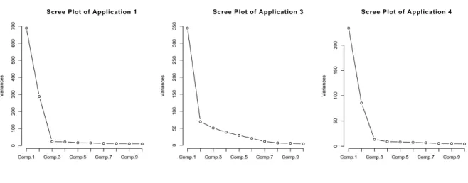
forecasting results.
Scree Plot of Application 1 Scree Plot of Application 3 Scree Plot of Application 4
Figure 2.6: Scree Plots
Because the SVD forecasting approach assumes no probabilistic models, Shen and Huang (2008) propose a nonparametric bootstrap method to derive the prediction interval of the forecast. Using our data, we apply the same method by first bootstraping the errors from time series model (2.17), and obtain the series {βˆTb+1,1,· · · ,βˆbT+1,K}, 1 ≤ b ≤B, where B is the number of bootstrap samples. Then by bootstrapping the errors in the forecasting model (2.18), we obtain B forecasts of xT+1. For an upper bound of the 95% prediction interval,
we use the end point of the 97.5% empirical percentiles of {x1T+1,· · ·, xBT+1}, and denote that estimate by ˆx(4)T+1.
Note that the SVD method involves regression on the decomposed data matrix, which is not efficient when the historical arrival volumes are close to zero. This happens to be the case for applications ranked 100 and lower in terms of total requests, whose hourly arrival rates are usually less than one. We therefore pool the lower ranked applications into few groups, and forecast the aggregated arrival rates within each group. We then split the forecasted group total arrival rates using the Bernoulli splitting rule, and obtain the hourly arrival rates for each individual application.
In the rest of the chapter, we useλ(n,ij) to denote the forecasted arrival rate of applicationn
2.6 Numerical Experiment
In this section, we report on the numerical experiments conducted to implement and com-pare the performance of the dynamic SAP using the three queueing models. The first queueing model (M/G/c/c) assumes that the arrival process is Poisson over each period. We use sta-tistical tests from Brown et al. [2005] to validate this assumption, and show that overall there is no evidence to reject the null hypothesis that the arrival process is NHPP with piecewise constant (PC) arrival rates. See Appendix A.1.3 for details. This PC arrival rate function can also be used in the dynamic SAP calculation with theM(t)/G/∞ model.
To implement the dynamic SAP, we forecast arrival ratesλn,iusing the methods introduced in Section 2.5. We assume that the mean service timessn,i are time-independent and simply take the sample mean sn for application n as the estimate of sn,i for all the periods. The approaches we use to estimate other parameters such as θn,i,pn,i of theMX/M/∞ queue are introduced later.
We simulate the system with the trace data from the VCL to compare the efficacy of all the methods introduced earlier. Each simulation setup can be described by four attributes described below:
Attribute 1. Forecasting Method: MA vs. SVD;
Attribute 2. Forecasting Level: Mean vs. upper bound of 95% prediction interval; Attribute 3. Estimation Method: SIPP vs. SDPP;
Attribute 4. Queueing Model: M/G/c/cqueue vs. MX/M/∞queue vs. M(t)/G/∞ queue. Thus there are a total of 2×2×2×3 = 24 simulation setups.
As a general parameter setting, we assume the targeted global probability of delay α∗ is 5%, and the targeted global blocking probability β∗ is 0.1%. There are 400 dedicated pools and one flexible pool. To forecast the arrival rates, we choose the length of rolling horizon
w = 30 days, and assume that there are P = 24 hourly periods in a day. Applying methods described in Section 2.5 for each application, we obtain four different sets of forecastsλ(1)n,i and
service times of applicationn, and we set loading timeun= 5 mins for all the applications. To determine the number of servers assigned over the ith interval, we letτi =i−1 (i≥1, in hours), and record the number of type-n users using the dedicated servers (Bn(i−1)) and the flexible servers (Fn(i−1)) at the end of the earlier period. Then the SIPP method and the SDPP method yield the following estimates:
ˆ
λn,i=λ(n,ij),
ˆ
λmod(n,i)= [λ (j)
n,i+Bn(i−1) +Fn(i−1)]/(1 +sn).
2.6.1 M/G/c/c Queue.
In this case, all of the estimated arrival rates are used directly as the input to the greedy algorithm of Section 2.4.2.1. We record the numbers of users blocked from all of the dedicated pools (overflows) and use them to forecast the arrivals to the flexible pool. The same procedures are used as those applied to the dedicated pools. The simulation results are presented in Figure 2.7.
The three plots on the left show the results using the mean forecasting level, while that right ones use the upper bound of 95% prediction interval. Panels (a) and (b) show the average probability of delay over the 24 hours in a day. We see that using the SVD forecasting method produces lower probabilities, and SDPP outperforms SIPP. In panel (a) we find all of the results are above the target level ofα∗ = 5%, which means our policies underestimate the number of servers needed. With the upper bound of 95% prediction interval, in panel (b), the two curves using the MA forecasting methods again fail to meet the target level. The other two curves using the SVD forecasting method are very close to, and hit our target 5% during the off-peak hours (3am-8am), but during the peak hours, the probability of delay goes up to 9%.
We also plot the average number of on servers (dedicated + flexible) over the 24 hours in Figure 2.7(e) and (f). Policies using the SVD forecasting method usually allocate more servers during the off-peak hour, which explains the lower probabilities of delay in (a) and (b). Besides, SDPP methods require less on servers than SIPP, while achieving the similar performance as shown in panel (b). Hence, for this queueing model, considering Attributes 1-3, we recommend the upper bound of 95% prediction interval as forecasting level, SDPP method, combined with SVD for dedicated pools and MA for flexible servers.
2.6.2 MX/M/∞ Queue.
Letσ2n,i be the variance of the number of arrivals. From Eq. 2.7 and 2.8 we see that
pn,i= 2/(
σn,i2 λn,i
+ 1), (2.19)
θn,i=λn,ipn,i,
which suggests,
rn,i=λn,isnpn,i/(1−pn,i).
Note thatQd(dn,i, rn,i) is a function ofrn,iand pn,i, and hence can be viewed as a function of λn,i and pn,i. Again we estimate λn,i using one of the combinations of our forecasting and estimation methods, while we estimate pn,i separately by computing the sample mean and variance of the corresponding hourly arrivals of the preceding 30 days, before plugging it into Eq. 2.19.
Furthermore, for a small fraction of the cases where pn,i >0.99, we use the Erlang-B loss formula to approximate the blocking probability instead of Eq. 2.9 to avoid computational instability. This makes sense since the Poisson distribution is the limiting case of the negative binomial distributionN B(r,1−p) when p→1 (or equivalently, asr→ ∞).
We collect the historical hourly overflow to the flexible pool and estimateλf,iandpf,iin the same way as for the dedicated pools. These parameters can also be computed using Eq. 2.10 and 2.11.
they are quite similar to those shown in Figure 2.7. (See Appendix A.1.4 for the corresponding figure.) Again, we find that the best policy uses 95% forecasting level, SDPP, combined with SVD forecasting for the dedicated pools and MA forecasting for the flexible pool. We will present the differences among the various queueing models (Attribute 4) later in Section 2.7, by using the same Attributes 1-3 for all queueing models.
2.6.3 M(t)/G/∞ Queue.
In this case, we first obtain the arrival function λn,i(t) by formulating a piecewise linear function using the hourly estimates ˆλn,i (or ˆλmod(n,i)). Then we approximate the CDF of the
service time of each application by its own empirical CDF. Finally we compute the integral in Eq. 2.12 numerically, and obtainmn(t), the mean number of busy servers of application nat timet. We use the same techniques for the flexible pool as in the case ofM/G/c/cqueue. We arrive at the same conclusion in comparing Attributes 1-3. See Section 2.7 for the comparison among the three queueing models.
2.7 Recommendations
Combining the results from the 24 simulation setups, we make the following recommenda-tions about the server allocation plan for the VCL:
(1) The SVD forecasting method results in a higher service quality than the MA for the dedicated pools. This can be explained by the time series model used in the SVD method, which include the day of week effects and the correlation within days. However for the more complicated arrival process in the flexible pool, the MA method simplifies the forecasting procedure and achieves better service quality.
service level (probability of blocking).
(3) The SDPP approach is highly recommended over the standard SIPP: our results show that SDPP always provides lower probability of delay while using significantly fewer servers (see Panel (f) in Figure 2.7). This is expected since SDPP incorporates the most recent data from the system to update the decision for the next period. Fortunately, SDPP is only slightly more computationally intensive than SIPP.
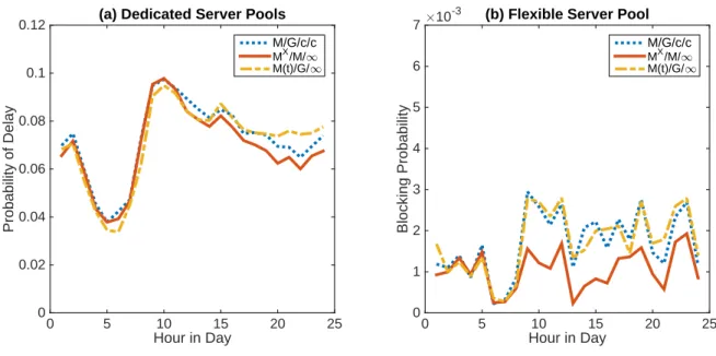
(4) To compare the three queueing models, we plot their performance in Figure 2.8 using the above recommended approaches: the upper bound of the 95% prediction interval, SDPP, combined with SVD for the dedicated pools and MA for the flexible pool. The figure shows that for the dedicated pools (Panel (a)), the performances of the three queueing models are quite similar. Since theM/G/c/cqueue is the most computationally efficient model, we recommend to use this model to quantify the probabilities of delay in the dedicated pools. For the flexible pool (Panel (b)), we recommend theMX/M/∞queueing model, which is a good approximation to the MX/M/c/c queue. Since the flexible pool is essentially accommodating the aggregate overflows from all of the dedicated pools, the over-dispersion issue is more obvious, which is taken care of by the CPP of theMX/M/∞queue model. The observations from the simulation results indeed show lower blocking probabilities than those obtained using the other queueing models.
2.8 Summary and Extensions
We then consider two methods – MA and SVD – to forecast future arrival rates given historical data, at two forecasting levels: the mean level and the upper bound of the 95% prediction interval level. We evaluate the performance of the dynamic SAP by conducting discrete event simulation experiments. We run statistical tests to justify the assumption of the piecewise constant arrival rate function over the planning horizon.
Overall, our recommended dynamic SAP keeps no more than 300 servers on during the peak hours and about 150 servers on during the off-peak hours, which is a significant saving over the 700-900 servers currently being kept on by the VCL using its policy. Furthermore, under our policy, at least 90% of the users receive immediate service from the dedicated server pools, and 99.9% of them are guaranteed a service from the flexible pool with no more than 5 extra minutes of waiting.
Figure 2.7: Simulation Results ofM/G/c/c Queue
Hour in Day
0 5 10 15 20 25
Probability of Delay
0 0.05 0.1 0.15 0.2 0.25 0.3 0.35
Mean Forecasting Level (a)
SIPP, MA SDPP, MA SIPP, SVD
SDPP, SVD
Hour in Day
0 5 10 15 20 25
Probability of Delay
0 0.05 0.1 0.15 0.2 0.25 0.3 0.35
Upper Bound of 95% Forecast Interval (b)
SIPP, MA SDPP, MA SIPP, SVD
SDPP, SVD
Hour in Day
0 5 10 15 20 25
Blocking Probability 0 0.005 0.01 0.015 0.02 0.025 0.03 0.035 0.04 0.045 (c)
Hour in Day
0 5 10 15 20 25
Blocking Probability
#10-3
0 1 2 3 4 5 6 7 (d)
Hour in Day
0 5 10 15 20 25
Average Number of ON Servers
0 100 200 300 400 500 (e)
Hour in Day
0 5 10 15 20 25
Average Number of ON Servers
Figure 2.8: Comparison of Three Queueing Models
Hour in Day
0 5 10 15 20 25
Probability of Delay
0 0.02 0.04 0.06 0.08 0.1
0.12 (a) Dedicated Server Pools
M/G/c/c MX/M/1 M(t)/G/1
Hour in Day
0 5 10 15 20 25
Blocking Probability
#10-3
0 1 2 3 4 5 6
7 (b) Flexible Server Pool
CHAPTER 3: Staffing and Scheduling for Health Care Facilities with Series Patients: Model I
3.1 Introduction
The United States spends more per capita on healthcare than many other developed coun-tries, and also has one of the highest growth rates on health care spending. The health care sector recently accounted for 17.3% of the GDP. The Institute of Medicine, in a recent report, estimated$750 billion in unnecessary health spending in 2009 alone, of which $130 billion has been attributed to inefficient delivery of care. There is a large opportunity for health care organizations to improve efficiency, quality, and timeliness of delivery of health care.
A healthcare organization’s appointment scheduling system can affect both timeliness of access to health services, as well as the efficiency of the healthcare operation. Timely access to a healthcare service is important from a clinical perspective, as well as from a patient satisfaction perspective. Scheduling systems also have the goal of matching demand with capacity in order to utilize resources efficiently. An appointment schedule also regulates the demand, i.e., patients visits, so as to minimize cost of operation.
While there has been significant research in the area of patient scheduling (see Smith-Daniels et al. (1988), Cayirli and Veral (2003), and Gupta and Denton (2008) for excellent surveys), most of prior literature has focused on scheduling patients with single appointments. Repeat visits by patients are usually treated in such models as distinct and independent visits. Our research focuses on determining capacity and scheduling “series” patients. Series patients are patients who need to be scheduled for multiple visits. In our research, we focus on specialty care clinics with such series patients. The issue of series patients arises in several specialty health services such as physical therapy, radiotherapy/chemotherapy for cancer, kidney dialysis, diabetes treatment, orthodontic treatment (braces), etc.
for repeated visits. At the beginning of the day, a batch of patient referrals is delivered from hospitals to a specialty care clinic. A clinic administrator contacts each patient and tries to schedule a first appointment for an initial examination. The health network with whom we interacted with requires that an initial evaluation examination should be scheduled within 48 hours from referral. In the case that there is appointment slot available for a new patient in this time window, the patient’s first examination is scheduled. Once he or she is evaluated, the plan of care for the patient is specified by a physician. The plan of care determines days between subsequent visits, total number of visits, and duration of each visit. Based on the plan of care, an administrator in the clinic generates an appointment schedule. The frequency, duration and length of the appointment time for the follow up visits vary greatly depending upon the patient’s diagnosis and/or specific needs as well as the physician order. Follow up visits are to be scheduled in a timely manner as well (2-3 days after the evaluation).
The health network we interacted with is currently unable to appropriately and consistently match supply and demand of physical therapy services. Each new patient creates a string of follow up visits. The follow up visits absorb a lot of the capacity on the schedule, making it difficult to get new patients in within the 24-48 hour required time frame at this health network. Thus, they are not able to consistently get new patients scheduled within 24-48 hours of referral. Many times, they are not able to consistently offer timely follow up appointments to their patients.
The primary goal of a our work is to devise a model for matching supply and demand through scheduling, as well as determining capacity, for a health service area that has series patients. Our model determines appropriate capacity to meet the demand of new patients (in the required time frame) as well as recurring visits (in the required time frame). We incorporate both revenue considerations as well as regular and overtime staffing costs in our model.