Sullivan, MJP
and
A.Thomsen, M
and
Suttle, KB
(2016)Grassland responses
to increased rainfall depend on the timescale of forcing. Global Change
Biol-ogy, 22 (4). pp. 1655-1665. ISSN 1354-1013
Downloaded from:
http://e-space.mmu.ac.uk/624025/
Version:
Accepted Version
Publisher:
Wiley
DOI:
https://doi.org/10.1111/gcb.13206
Please cite the published version
1
Grassland responses to increased rainfall depend on the timescale of forcing
1
Running head: Contrasting responses to weather and climate
2
Martin J. P. Sullivan1*, Meredith Thomsen2, and K.B. Suttle3* 3
1. School of Geography, University of Leeds, Leeds, LS2 9JT, UK
4
2. Department of Biology, University of Wisconsin, La Crosse, Wisconsin 54601, USA.
5
3. Department of Ecology and Evolutionary Biology, University of California, Santa Cruz, CA 95064.
6
*Corresponding authors: Martin Sullivan, tel +44 (0) 113 34 31039, email: [email protected];
7
Blake Suttle, email: [email protected]
8
Key words: Prediction, Time Series, Correlation, Extrapolation, Trophic Level, Context, Climate
9
Change
10
Type of paper: Primary Research Article
11 12
2
Abstract
13
Forecasting impacts of future climate change is an important challenge to biologists, both for
14
understanding the consequences of different emissions trajectories and for developing adaptation
15
measures that will minimize biodiversity loss. Existing variation provides a window into the effects
16
of climate on species and ecosystems, but in many places does not encompass the levels or
17
timeframes of forcing expected under directional climatic change. Experiments help us to fill in these
18
uncertainties, simulating directional shifts to examine outcomes of new levels and sustained changes
19
in conditions. Here we explore the translation between short-term responses to climate variability and
20
longer-term trajectories that emerge under directional climatic change. In a decade long experiment,
21
we compare effects of short-term and long-term forcings across three trophic levels in grassland plots
22
subjected to natural and experimental variation in precipitation. For some biological responses (plant
23
productivity), responses to long-term extension of the rainy season were consistent with short-term
24
responses, while for others (plant species richness, abundance of invertebrate herbivores and
25
predators) there was pronounced divergence of long-term trajectories from short-term responses.
26
These differences between biological responses mean that sustained directional changes in climate
27
can restructure ecological relationships characterizing a system. Importantly, a positive relationship
28
between plant diversity and productivity turned negative under one scenario of climate change, with a
29
similar change in the relationship between plant productivity and consumer biomass. Inferences from
30
experiments such as this form an important part of wider efforts to understand the complexities of
31
climate change responses.
32 33
3
Introduction
34
Understanding how species and ecosystems respond to directional environmental changes is critical to
35
designing adaptation strategies that will maintain our ecological support systems through the current
36
period of global climate change. A useful starting point for investigating how the functioning of
37
ecosystems and the abundance and distribution of different species will respond to future climate
38
change is to ask how they have responded to the changes we have already seen (e.g. Johnston et al.,
39
2013, Kurz et al., 2008, MacNeil et al., 2010). A critical challenge is that the windows we have into
40
these impacts—natural climatic variability and the directional forcings apparent therein, experiments
41
simulating climate forcing, and directional changes in baseline conditions already evident—are
42
typically short in duration or small in magnitude relative to the climatic changes expected from
43
current emissions trajectories and resulting earth-surface energy imbalances. Ecologists must
44
therefore grapple with how responses to pulsed or small-magnitude changes relate to responses to
45
chronic and larger magnitude shifts (Shaver et al., 2000, Smith et al., 2009).
46
The translation between effects of short-term forcings and effects of sustained forcings is not always
47
linear or straightforward. Early field experiments simulating climate change found that certain
48
responses changed direction relative to controls through time (Chapin et al., 1995, Harte &Shaw,
49
1995), presumably owing to interactions among different species or groups of species. Changes in
50
climate can alter the strength and nature of ecological interactions, leading to indirect effects that alter
51
response trajectories and are often lagged relative to direct physiological responses (Forchhammer et
52
al., 2002, Smith et al., 2009, Suttle et al., 2007, Wiedermann et al., 2007). Thus species interactions
53
have been borne out as important drivers of non-linear responses to changing climate through a large
54
body of research (reviews in Cahill et al., 2012, Ockendon et al., 2014, Shaver et al., 2000, Walther,
55
2010), even as they have come to be understood as one class of a suite of such drivers. Physiological
56
thresholds and tipping points can likewise cause ecological trajectories to deviate in sudden and
57
unexpected ways under sustained or larger-magnitude forcing that are not apparent from itinerant or
58
smaller forcing (Grottoli et al., 2014, Kirby & Beaugrand, 2009, Kortsch et al., 2012, Nelson et al.,
59
2013). Species may acclimate to changing climate, so that initially pronounced effects taper off with
4
repeated exposure (Donelson et al., 2011, Grottoli et al., 2014, McLaughlin et al., 2014). Populations
61
may also adapt to selective pressures of changing climate (Colautti & Barrett, 2013, van Asch et al.,
62
2013). Each of these factors can cause long-term trajectories under sustained climate forcing to
63
deviate from short-term effects of initial or itinerant forcing. Understanding the causes of these
64
deviations, the urgent question becomes whether being able to identify these complexities and
65
quantify their effects advances us toward practical improvements in predictive capability.
66
We can build biotic interactions, physiological thresholds, acclimation and adaptation into predictive
67
models to account for their effects on target variables (e.g. Coulson et al., 2011, Fordham et al., 2013,
68
Heikkinen et al., 2007, Luoto et al., 2007, Trainor & Schmitz, 2014, Trainor et al., 2014), so much of
69
the challenge we face is to understand when this is actually needed: under what contexts, in what
70
ecosystem types, and for what response variables do the different factors emerge to strongly influence
71
the shape of responses? Progress toward the development of conceptual frameworks to address these
72
questions is already underway. Drawing on a number of field experiments in different ecosystem
73
types around the world, Shaver and colleagues (2000) delineated the various direct and indirect effects
74
of temperature change on ecosystem carbon budgets, illustrating how the balance among these
75
different processes can change through time to produce multi-phase responses. The authors showed
76
how experiments can be used to identify dominant mechanisms governing different phases of
77
response and the transitions between them. Subsequent research has built upon these ideas to develop
78
a general framework to organize drivers of multi-phase responses into a predictable sequence (Smith
79
et al., 2009). Smith and colleagues outline a temporal hierarchy of mechanisms governing ecosystem
80
responses to climate change that facilitates prediction of non-linear responses through time. This
81
hierarchical-response framework places physiological responses of individuals, reorganization of
82
species within a community, and turnover of species across communities into a logical temporal order
83
with respect to sustained environmental forcing. By organizing drivers of ecosystem responses to
84
climate change into explicit sequences, both approaches focus attention around controls on
non-85
linearity in responses and how we might generalize these according to starting conditions, response
86
type, and ecosystem type.
5
We now well understand that responses to pulsed climatic forcings and moderate directional changes
88
in the observed record may be poor predictors of future ecological changes under sustained global
89
climate change, and we are making progress toward understanding how and why responses to the
90
more chronic directional forcing may change direction through time. The possibility that we may be
91
able to sort the complexity of such responses according to ecosystem type, species or ecosystem
92
characteristics, or the type of response variable under focus provides a pathway to improved
93
prediction (Shaver et al., 2000, Smith et al., 2009) and encourages further study. Researchers have
94
already produced evidence of such sorting by ecosystem type: a recent meta-analysis found
95
herbaceous systems tend to show continuous directional ANPP responses to global change drivers
96
while stepped responses are more common in forests and other systems (Smith et al., 2015). In the
97
present paper, we consider how predictability varies with the type of response variable under focus.
98
We used watering amendments in a northern California grassland to push the annual rainy season to
99
the tails of existing variability in either intensity or duration, in order to test how well effects of
100
background variation predict effects of sustained forcing. From ten years of data on plant production
101
and richness and on herbivore, predator, and parasitoid abundances, we examine the translation
102
between short-term responses of each variable to both background variation and initial years of rainy
103
season modification and to long-term trajectories under sustained changes in the rainy season.
104 105
Materials and Methods
106
Natural History of the Study System
107
Research was undertaken in a 2.7-hectare grassland at the Angelo Coast Range Reserve in Mendocino
108
County, California (39˚ 44’ 17.7” N, 123˚ 37’ 48.4” W) (Suttle et al., 2007). Part of a network of 39
109
natural areas protected across the state for research and teaching by the University of California’s
110
Natural Reserve System, the Angelo Reserve consists predominantly of mixed-oak woodland and
old-111
growth conifer forest surrounding headwater streams of the South Fork Eel River. Grassy meadows
6
are interspersed within the forest on abandoned river terraces, with vegetation consisting of a
well-113
mixed assemblage of grasses and forbs of both native and exotic origins.
114
The region experiences a Mediterranean-type climate, with hot dry summers and cool wet winters.
115
Annual rainfall averages 2160 mm and falls predominantly between October and April. Seasonal
116
precipitation levels have a well-established role in structuring annual patterns of plant production and
117
composition in California grasslands. Successional dynamics are generally not apparent in these
118
systems, and production and composition instead vary non-directionally from year to year according
119
to annual climatic variation – and particularly the timing and amount of precipitation that falls each
120
year (Hobbs et al., 2007, Pitt & Heady, 1978, Stromberg & Griffin, 1996).
121
Between 20 and 40 vascular plant species are present in the grassland in a given year. Annual grasses
122
of Mediterranean origin typically make up the major share of ground cover, with populations of three
123
native perennial bunchgrass species and numerous native and exotic forbs co-existing with the exotic
124
grasses.
125
Experimental Design
126
Since January 2001, thirty-six 70m2 circular plots have been exposed to one of three water 127
amendment treatments assigned in a randomized block design. Treatments consist of an ambient
128
control, a wintertime addition over ambient precipitation that simulates an intensified rainy season,
129
and a springtime addition over ambient that simulates an extended rainy season. The Intensified rainy
130
season treatment and the Extended rainy season treatment were developed to approximate projections
131
for the region from leading climate models at the time the experiment was initiated (National
132
Assessment Synthesis Team, 2000). Models from both the Hadley Centre for Climate Prediction and
133
Research and the Canadian Centre for Climate Modeling and Analysis projected substantial increases
134
in annual rainfall for coastal northern California by mid-century, with the Hadley model (HadCM2)
135
calling for the entirety of the increase during the existing winter rainy season and the Canadian model
136
(CCM1) calling for an extended rainy season into the spring and summer.
7
Each watered plot received approximately 440 mm of supplementary water over ambient rainfall each
138
year, representing roughly a 20% increase over mean annual precipitation but within the range of
139
natural variability in both amount and timing at the study site (details in Suttle et al., 2007). Water is
140
collected from a natural spring on a forested slope immediately to the east of the grassland, with a
141
portion of its flow filtered to 40 microns and diverted via irrigation piping to a 4500-liter irrigation
142
tank placed approximately 40 vertical meters upslope of the meadow. The tank is continually
143
replenished via gravity-feed from the spring, and water has been tested and found to contain nitrogen
144
concentrations within the range present naturally in rainwater at the study site (Suttle et al., 2007).
145
Water is delivered evenly over the surface of each plot from a single RainBird® RainCurtain™
146
sprinkler (Rainbird, Azusa, CA USA) in the center of each plot. The water delivery protocol is
147
identical for the Intensified and Extended rainy season treatments, except that the applications are
148
staggered by three months, with the Intensified rainy season addition running from January through
149
March and the Extended rainy season addition running from April through June. Experimental rain
150
additions begin approximately two hours after dawn every third day. Valves leading to the sprinklers
151
are actuated by battery-operated timers set to “rain” 14 to 16 mm of water onto the plots over one
152
hour. The watering radius is 5m, and all samples are collected at least 0.5m in from the outside edge
153
of the watered area, as described under Response Variables below.
154
Ambient precipitation throughout the study was measured with automated Campbell sensors located
155
at two different meteorological monitoring stations in grasslands on the reserve. Where occasional
156
sensor faults led to missing data, precipitation estimates were interpolated from nearby weather
157
stations in Laytonville (39.7023, -123.4849; R2= 0.727), or, when data from Laytonville were not
158
available, from Eel River (39.8253, -123.0825; R2= 0.398) based on regression equations from
159
surrounding days when sensor data were available for both the Angelo Reserve and these stations
160
Approximately 90% of daily precipitation totals for the ten-year record from 2001 through 2010 come
161
directly from weather stations at the Angelo Reserve, with the remaining 10% interpolated.
162
Response Variables
8
In 2000, prior to initiation of the watering amendments, eighteen plots were partitioned for concurrent
164
long-term measurements of plant production, plant diversity, and invertebrate abundances (Fig. S1).
165
The remaining eighteen plots were set aside for other work not part of this study, so that all data
166
reported here are from six replicates of each of the three watering treatments.
167
Plant production was measured from biomass samples collected three times each growing season from
168
two separate pre-designated 0.09 m2 subplots. Samples were taken on or around 20 May, 1 July, and
169
30 August, dates that collectively target the peak biomass of each different species in the system. All
170
vegetation was clipped at the soil surface, sorted into eight functional/phenological groups (spring
171
annual grass, summer annual grass, perennial grass, spring annual forb, summer annual forb,
late-172
summer annual forb, perennial forb, and nitrogen-fixing forb) and dried at 72oC for 48 hours prior to 173
weighing. Each species was included once in ANPP estimates for each year. Each subplot was
174
harvested in this manner only once and then eliminated from the future sampling scheme. A five-year
175
allotment of subplots (i.e. 30 total, with six subplots sampled per plot each year) was laid out at
176
regular intervals along two parallel transects running in a randomly drawn cardinal direction through
177
the centre of each plot, and an additional five years allotment was arrayed along two transects
178
perpendicular to this first set (see Figure S1). Plant production was estimated by summing the
179
biomass of each different functional-phenological group at its annual peak biomass. Litter was not
180
included in ANPP estimates.
181
Plant diversity was measured as the mean species richness of two central 0.25 m2 subplots in each 182
plot. Diversity subplots were surveyed regularly over the growing season to account for phenological
183
differences in the seasonal growth patterns of different species.
184
Invertebrate abundances were sampled on or around 1 August every year. Foliar and flying
185
invertebrates were sampled via a 30.5 cm diameter sweep net modified to connect securely to a
186
holding container open at the base of the net. Samples were collected by a quick succession of ten
187
sweeps along a transect running through the centre of the plot and then a second set of ten sweeps
188
running back through the plot along a perpendicular transect (at 45˚ offsets from transects for biomass
9
clips). Sample containers were immediately capped after the last sweep and then frozen until sorting.
190
Ground-dwelling invertebrates were sampled over 48 hours in 5cm diameter pitfall traps. Prior to
191
initiation of the experiment in 2001, two 15cm sections of hollow rubber pipe (diameter 5.2cm) were
192
sunk vertically into the soil in opposite quadrants in each plot, using a sledge hammer to anchor each
193
approximately 1cm below the soil surface. Into each section of pipe was placed a capped plastic
194
container of 5cm diameter, suspended from the top of the pipe by a lip at the top of each container
195
onto which the cap secured. To initiate a pitfall sample, caps were removed and the open containers
196
suspended in each pipe just below ground surface were filled to 2cm depth with a dilute solution of
197
water and unscented dish soap. This minimized soil and vegetation disturbance immediately prior to
198
collection and any biases that could result. Upon collection, invertebrates were transferred into vials
199
of 70% ethanol for storage until sorting, and the pitfall traps were recapped in place in the plots.
200
Invertebrates were identified to family, with morphotypes sorted within families. Replicate
201
specimens of each morphotype were weighed for plot-wise biomass estimations. Invertebrate families
202
were assigned to herbivore, predator, and parasitoid feeding groups based on natural history records.
203
Hypothesis Tests and Statistical Analyses
204
All statistical analyses were carried out within a mixed effects model framework, implemented in R
205
(R Core Team, 2014) using the package lme4 (Bates et al., 2014). Invertebrate abundances were
206
modelled using a Poisson error structure and log link. All responses were modelled using plot identity
207
as a random effect to account for the repeated measurements from each plot, where factors such as
208
soil texture and seed bank could lead to correlation among measurements. For invertebrates,
within-209
year correlations between observations could arise from site-wide responses to weather, so
210
invertebrate responses were modelled with year as a random effect to account for this. Both year and
211
plot identity random effects were specified as random intercepts, where year and plot identity are
212
crossed grouping factors. In total there were 180 observations of each response variable, collected in
213
18 plots over ten years.
10
Analyses focused on testing how well responses to short-term forcings predicted responses to the
215
same forcings applied over longer terms. We consider two different kinds of short-term forcing: (1)
216
natural anomalies in rainfall that entailed seasonal precipitation levels within the range experienced by
217
the water addition treatments (between 326 mm and 380 mm above long-term means for each season);
218
and (2) experimental amendments that delivered seasonal precipitation levels 440 mm greater than
219
long-term means in the first two years of the experiment. Two years was chosen as a threshold for
220
dividing short- and long-term responses as it allows both initial responses and lagged effects of
221
precipitation in the previous year to be observed, but did not include evident indirect effects that
222
became pronounced in the third year and thereafter (Suttle et al., 2007). Longer-term forcings were
223
then defined as the subsequent years in the Intensified (Int) and Extended (Ext) rainy season
224
treatments (Years 3-10). Using control plots for baseline levels, and the forcings provided by natural
225
rainfall anomalies and the experimental manipulations, we were able to conduct a four-way
226
comparison for each scenario of rainy season change (Table 1). Each response variable was modelled
227
as a function of forcing type (i.e. control, short-term natural variation, short-term experimental
228
manipulation and long-term experimental manipulation), with separate models for each rainy season
229
change scenario. Post-hoc tests implemented in the R package multcomp (Hothorn et al., 2008) were
230
used to test for significant differences between each forcing type. Full details of these models are
231
given in Table S1, with full results of post-hoc tests given in Table S2.
232
To ensure our results are not affected by the choice of timescale for dividing short-term and long-term
233
responses we also analysed the dataset treating time as a continuous variable. In this analysis, each
234
response variable was modelled as a function of experimental treatment (Int, Ext or Control), year
235
since the start of the experiment and the interaction between treatment and year. A significant
236
treatment-year interaction in the opposite direction to the effect of treatment would indicate differing
237
short-term and long-term responses to that treatment. Full details of these models are presented in
238
Table S3.
239
We examined whether precipitation addition changed relationships between plant diversity and plant
240
productivity and between plant productivity and consumer biomass by modelling the variable thought
11
most likely to be the response variable in each relationship (plant productivity and consumer biomass
242
respectively) as a function of the corresponding explanatory variable (plant species richness and plant
243
productivity respectively), precipitation addition treatment and their interaction. A significant
244
interaction with treatment would indicate that the slope of these relationships changed under certain
245
precipitation addition treatments.
246 247
Results
248
Intensification of the winter rainy season had only minor effects on plant production (Figs. 1a, 2a),
249
with no overall effect of the Int treatment (t = 1.64, P = 0.108). The interaction between Int and Year
250
was not significant (t = 0.53, P = 0.598), indicating that the effect of rainy season intensification did
251
not change with the duration of forcing. Higher plant production in the later years of the Int treatment
252
(Int1,2 vs Int3-10: z = 3.81, P < 0.001, Fig. 2a) likely reflects a weak but significant increase in primary 253
production across treatments during the experiment (Year effect: t = 2.23, P = 0.03, Fig. 1a). Plant
254
production in control plots did not significantly change in years with naturally elevated winter
255
precipitation (C vs Cint:z = 1.34, P = 0.526). In contrast, experimental extension of the rainy season 256
significantly increased plant production (Ext effect: t = 4.72, P < 0.0001). The effect of rainy season
257
extension did not change with the duration of forcing (Fig. 2b), with no significant differences in
258
short-term and long-term responses (Ext1,2 vs Ext3-10: z = 0.35, P = 0.984) nor significant interaction 259
between Ext and Year (t = 0.31, P = 0.757). Plant production responded positively but
non-260
significantly to naturally extended rainy seasons (C vs Cext: z = 1.18, P = 0.622). 261
Plant species richness was significantly depressed in years with naturally intense winter rainy seasons
262
(C vs Cint: z = 3.54, P = 0.002, Fig. 2c), but showed no response to experimental intensification of the 263
rainy season (Int effect: t = 1.42, P = 0.163). The effect of Int did not change with duration of forcing
264
(Int1,2 vs Int3-10: z = 0.39, P = 0.979; Int – Year interaction: t = 1.21, P = 0.233). In contrast, the short-265
term and long-term response of plant species richness to extension of the rainy season was
266
significantly different (Ext1,2 vs Ext3-10: z = 8.70, P <0.0001; Ext – Year interaction: t = 6.49, P < 267
12
0.0001), with a non-significant but positive effect of natural and experimental short-term extensions
268
of the rainy season contrasting with a significant negative effect of repeated extensions of the rainy
269
season (Figs. 1a, 2d).
270
Invertebrate herbivores showed little abundance response to intensified winter rainy seasons (Fig. 3a),
271
with no significant differences evident from the control treatment in years of more typical winter
272
rainfall (comparisons of Cint, Int1,2 and Int3-10 with C: z ≤ 1.35, P ≥ 0.508). These herbivores showed 273
pronounced responses to an extended rainy season (Fig. 3b), however, with large increases in
274
abundance in years of naturally high April, May, and June precipitation (C vs Cext, z = 6.42, P 275
<0.0001) and in Ext treatment plots in the initial years of the study (C vs Ext1,2: z = 7.99, P <0.0001). 276
Responses to rainy season extension changed with the duration of forcing (Ext1,2 vs Ext3-10: z = 5.66, P 277
< 0.0001; Ext –Year interaction: z = 5.00, P < 0.0001), with herbivore abundances in Ext3-10 plots 278
similar to those in control plots (Figs. 1b, 3b).
279
Predators followed the same pattern as herbivores (Figs. 1b, 3c, 3d), with no evident responses to
280
intensified winter rainy seasons (comparisons of Cint, Int1,2 and Int3-10 with C: z ≤ 1.60, P ≥ 0.358 , and 281
strong positive responses to the extended rainy season treatment (C vs Ext1,2: z = 5.97, P < 0.0001) 282
that diminished when this regime was sustained across years (Ext1,2 vs Ext3-10, z = 4.18, P = 0.0002; 283
Ext – Year interaction: z = 2.16, P = 0.031). Natural extensions of the rainy season had a
non-284
significant positive effect on predator abundance (C vs Cext: z = 1.63, P = 0.353). 285
Neither intensification nor extension of the rainy season significantly altered parasitoid abundance (z
286
≤ 2.28, P ≥ 0.091), although the weakening of the positive response to Ext with sustained forcing
287
echoed the responses of herbivores and predators. Parasitoid abundance declined during the
288
experiment across all treatments (Year effect: z = 3.81, P = 0.0001, Fig. 1b).
289
Plant species richness and plant production were positively related in both control and Int plots (β =
290
5.034 ± 1.904 SE, t = 2.64, P = 0.0097, Fig 4a). Initial positive responses in plant species richness and
291
plant production to experimental extension of the rainy season (Fig. 2b) did not alter the direction of
292
this relationship (Fig. S1a: years 1 and 2). However, as the long-term response of plant richness to
13
extended annual rainy seasons turned from positive to sharply negative (Fig. 2d), so over time did the
294
direction of the relationship between plant species richness and plant production in these plots (Fig
295
S1a, years 3 to 10). Thus extension of the rainy season, when sustained across years, turned the
296
positive relationship between diversity and production in the grassland system negative (significant
297
interaction between effect of plant species richness and Ext, t = 2.83, P = 0.0057, Fig. 4a). Plant
298
production and consumer biomass (natural log transformed) were positively related in control and Int
299
plots (β = 0.004 ± 0.001 SE, t = 3.52, P = 0.006). However, a significant interaction with Ext (t =
300
2.43, P = 0.0166) meant that this relationship was not evident under extension of the rainy season
301
(Fig. 4b). This interaction effect was not lagged (Fig. S1b).
302 303
Discussion
304
We find that responses to short-term forcings are reliable predictors of trajectories under longer-term
305
forcing in some variables but not others. Thus measurements taken under background variability at
306
the study site or from a short-term experiment would reliably predict effects of more sustained
307
directional climatic changes in certain variables, but would mislead us as to expected changes in other
308
variables. In keeping with the pattern documented in a recent cross-ecosystem synthesis (Smith et al.,
309
2015), we find a consistent directional response in ANPP even as species composition in the extended
310
rainy season treatment shifted. Response variables of plant species richness and invertebrate
311
abundances, however, showed greater complexity, with the notable consequence of reshaping
312
relationships between plant production and diversity and between primary and secondary production
313
in the system.
314
There are many factors that can cause long-term trajectories under directional climate forcing to
315
deviate from responses to shorter-term forcings: physiological thresholds, species interactions,
316
acclimation, and adaptation can all introduce non-linearities into ecological responses (Grottoli et al.,
317
2014, Ockendon et al., 2014) as can differences in the time these processes take to manifest
318
themselves (Smith et al., 2009). The challenge for ecological prediction is that the influence of these
14
factors can be context specific, depending on environmental conditions and the specific variable under
320
consideration (e.g. Voigt et al. 2003). Thus in our study, not only were long-term effects in line with
321
the direction of short-term effects in some variables while in opposite directions in others, but the
322
incidence of these discrepancies varied between the two scenarios of climate change tested.
Short-323
term responses of plant species richness, herbivore abundance and predator abundance to extension of
324
the rainy season differed from responses to sustained directional forcing. In contrast, we did not
325
detect any stark misalignments between short-term and long-term effects of intensified winter rainy
326
seasons, where effects were generally much weaker overall than effects of extended rainy seasons.
327
Where short-term experimental water addition had a statistically significant effect (i.e. responses of
328
plant production, herbivore abundance and predator abundance to extension of the rainy season),
329
responses to natural rainy season variation were always in the same direction as responses to
330
experimental water addition, but were weaker and only statistically significant for herbivore
331
abundance (Fig. 3b). In contrast, we measured significant declines in plant richness in years with
332
particularly intense winter rainfall, but did not detect any such effect in plots subjected to
333
experimental rainy season intensification (Fig. 3c). Differences in responses to natural and
334
experimental short-term forcing demonstrate the importance of the context and manner in which
335
forcings are applied. Our basis in comparing natural rainy season anomalies with systematic
336
experimental additions was equivalency of total amount, not accounting for differences in frequency
337
and duration of rainfall events, or for other factors such as total insolation or average temperature,
338
which could also have some ecological effect. It is further possible that legacy effects, interannual
339
variation in precipitation outside of our focal seasons and variation in climatic conditions besides
340
precipitation affected response variables. With 10 years of data it is not possible to disentangle the
341
effects of these variables, however increases in plant production, herbivore abundance and predator
342
abundance following a naturally extended rainy season in 2005 but not following similar conditions in
343
2003 (Fig. 1) illustrate their importance.
344
Differences in short-term and long-term responses to extended rainy seasons emphasize the
345
importance of species interactions in long-term ecological responses to climate change. The reversal
15
from initially (but non-significantly) positive to strongly negative responses in plant richness and the
347
changes from strongly positive to null responses in invertebrate consumers reflect the influence of
348
indirect effects from altered competitive and consumer-resource interactions. Research into the first
349
five years of data from this experiment showed that positive direct effects of extended rainy seasons
350
on nitrogen-fixing forbs favored improved performance by annual grasses, which then competitively
351
supressed broad-leaved forbs and due to their early senescence limited upward energy flow to higher
352
trophic levels (Suttle et al., 2007). Results reported here demonstrate that these indirect effects do not
353
represent short-term dynamics, but leave a strong legacy on system dynamics, with plant species
354
richness remaining suppressed in extended rainy season plots throughout the course of the experiment
355
and herbivores and predators remaining at significantly lower abundances than their initial responses.
356
Results at consumer trophic levels require more nuanced interpretation than responses by plants;
357
because plots were open to the surrounding grassland, measurements taken in experimental plots can
358
reflect patterns of aggregation and dispersion within the overall invertebrate populations existing in
359
the broader system. Thus abundances in water-addition plots better reflect aggregation or avoidance
360
based on treatment effects on the environment of those plots, while comparisons of year to year
361
changes in abundance in control plots (i.e. Cint Vs C and Cext vs C) mostly reflect net demographic 362
effects of a particularly intense or particularly extended rainy season relative to more typical rainy
363
season (along with any effects of the myriad other environmental conditions that vary among years).
364
These demographic effects can be seen in the positive responses of herbivores (and potentially in the
365
non-significant positive responses of predators) to naturally extended rainy seasons.
366
Positive responses of herbivores and predators (and a non-significant positive response of parasitoids)
367
to the initial experimental extension of the rainy season are likely to reflect aggregation to favourable
368
islands of habitat within the broader grassland. In the first year of the experiment, extended rainy
369
season plots were more productive and had higher species richness than control plots (Fig. 1), with
370
forbs, which previous work at the study site has shown to sustain a greater density of invertebrate
371
herbivores than annual grasses (Suttle et al. 2007), accounting for a greater proportion of primary
372
productivity (Fig. S3). As rainfall amendments were repeated across years, indirect effects of
16
extended rainy seasons increased the dominance of annual grasses and reduced plant species richness.
374
This appears to have made these plots no more favourable than the rest of the surrounding grassland
375
(Fig. 3). Notably, in the one year (2005) when plant production was comparable across all three
376
treatments, the abundance of herbivores and predators was lower in extended rainy season plots than
377
in other treatments (Fig. 1). This suggests that once differences in plant production were accounted
378
for, the lower plant species richness of extended rainy season plots had a negative effect on
379
invertebrate consumers, possibly due a reduction in the structural complexity of vegetation (Dennis et
380
al., 1998).
381
Although parasitoids showed a qualitatively similar response to rainy season extension as other
382
invertebrates, these responses were not statistically significant (Fig. 3). In part this could be due to
383
reduced statistical power to detect trends due to the lower abundance of parasitoids. Parasitoid
384
abundance did decline across the whole study system over the course of the experiment (Fig. 1). The
385
reasons for this are unclear, but as parasitoids are wide ranging (Rosenheim et al., 1989) this could
386
reflect meadow-wide consequences of the reduction in herbivore abundance in extended rainy season
387
plots.
388
Responses to water addition treatments are likely to be also influenced by factors other than seasonal
389
precipitation, such as legacy effects from the state of the system in previous years (Sala et al., 2012).
390
It is therefore possible that short-term responses to water addition would be different if they were
391
applied in a different year. As long-term responses were influenced by a number of species
392
interactions following initial water addition, it is also possible that any differences in short term
393
responses could influence the long-term trajectory of the system, adding further complexity to
394
predicting climate change impacts.
395
We turn to ecological time series encompassing climatic variability and to experiments simulating
396
climate change to gain insights into how forcings in different directions affect variables of interest.
397
Because the forcings manifest in background climate variability and extremes, in cyclical variation
398
accompanying large-scale oscillations such as El Nino and the NAO, and in short-term experimental
17
studies may not match the levels or timeframes of forcings that will accompany directional climatic
400
change, it is important to understand the translation of short-term effects into long-term trajectories.
401
The prevalence of thresholds, biotic interactions, acclimation, and adaptation in ecological responses
402
to climate change means that this translation may not be straightforward. Hence experimental results
403
can poorly predict natural patterns that develop over longer timescales (Sandel et al., 2010), initial
404
responses to experimental manipulations may poorly predict longer-term effects (Chapin et al., 1995,
405
Harte & Shaw, 1995, Hollister et al., 2005, Wiedermann et al., 2007), populations that show a strong
406
response to initial exposure to certain conditions may show little or no response over longer terms
407
(Donelson et al., 2011, Grottoli et al., 2014, McLaughlin et al., 2014, Shaver et al., 2000, Smith et al.,
408
2015), and populations that show little response to initial or itinerant exposure may show pronounced
409
responses to repeated or sustained exposure (Grottoli et al., 2014, Kirby & Beaugrand, 2009, Kortsch
410
et al., 2012) .
411
We find similar dynamics at work in our system, with little or no response to intensified rainy seasons
412
but both transient (invertebrate consumers) and continuous positive responses (plant production, cf
413
Smith et al. 2015) to rainy season extension, as well as responses that reverse in direction relative to
414
controls (plant species richness). Because long-term effects extended more straightforwardly from
415
short-term responses for some variables than for others, an important consequence was to alter basic
416
relationships between ecological variables. Rainy season extension had a persistent positive effect on
417
plant production, but its effect on plant diversity changed from (non-significantly) positive to strongly
418
negative over time, leading to a reversal in the relationship between plant production and diversity
419
through time as well. The form of this relationship is of considerable interest to conservation
420
planning, with focus on whether management actions that promote ecosystem services also benefit
421
diversity and vice versa (e.g. Hulme et al., 2013). In this study we found that a measure of diversity
422
(plant species richness) was positively correlated with plant production (a provisioning ecosystem
423
service) under ambient conditions and one scenario of directional climate change, and initially under
424
the other scenario of directional climate change, but the correlation turned negative over time. A
425
similar but less drastic change was evident for the relationship between plant production and
18
consumer biomass. That fundamentally different relationships can emerge between key ecological
427
variables under sustained forcing from those that prevail under ambient conditions further underscores
428
the need to consider evidence from multiple approaches and sources in planning for and managing
429
climate change impacts.
19
Acknowledgements
431
The experiment was established with funds from the US Environmental Protection Agency and the
432
Canon National Parks Sciences Scholarship Program. Support for the research was provided by US
433
National Science Foundation grant DEB-0816834, the US National Science Foundation’s National
434
Center for Earth Surface Dynamics, the California Energy Commission’s Public Interest Energy
435
Research program, the University of California at Berkeley, the University of Wisconsin at La Crosse,
436
and Imperial College London. MS is currently funded by the European Research Council grant
437
“Tropical Forests in the Changing Earth System”. We wish to thank Peter Steel and the University
438
of California Natural Reserve System for stewardship and protection of the study site.
439 440
20
References
441
Bates D, Maechler M, Bolker BM, Walker S (2014) Lme4: Linear mixed-effects models using eigen 442
and s4. pp Page. 443
Cahill AE, Aiello-Lammens ME, Fisher-Reid MC et al. (2012) How does climate change cause 444
extinction? Proceedings of the Royal Society of London B: Biological Sciences, 280. 445
Chapin FS, Shaver GR, Giblin AE, Nadelhoffer KJ, Laundre JA (1995) Responses of arctic tundra to 446
experimental and observed changes in climate. Ecology, 76, 694-711. 447
Colautti RI, Barrett SCH (2013) Rapid adaptation to climate facilitates range expansion of an invasive 448
plant. Science, 342, 364-366. 449
Coulson T, Macnulty DR, Stahler DR, Vonholdt B, Wayne RK, Smith DW (2011) Modeling effects of 450
environmental change on wolf population dynamics, trait evolution, and life history. Science, 451
334, 1275-1278. 452
Dennis P, Young MR, Gordon IJ (1998) Distribution and abundance of small insects and arachnids in 453
relation to structural heterogeneity of grazed, indigenous grasslands. Ecological Entomology, 454
23, 253-264. 455
Donelson JM, Munday PL, Mccormick MI, Nilsson GE (2011) Acclimation to predicted ocean warming 456
through developmental plasticity in a tropical reef fish. Global Change Biology, 17, 1712-457
1719. 458
Forchhammer MC, Post E, Stenseth NC, Boertmann DM (2002) Long-term responses in arctic 459
ungulate dynamics to changes in climatic and trophic processes. Population Ecology, 44, 113-460
120. 461
Fordham DA, Akcakaya HR, Brook BW et al. (2013) Adapted conservation measures are required to 462
save the iberian lynx in a changing climate. Nature Clim. Change, 3, 899-903. 463
Grottoli AG, Warner ME, Levas SJ et al. (2014) The cumulative impact of annual coral bleaching can 464
turn some coral species winners into losers. Global Change Biology, 20, 3823-3833. 465
Harte J, Shaw R (1995) Shifting dominance within a montane vegetation community: Results of a 466
climate-warming experiment. Science, 267, 876-880. 467
Heikkinen RK, Luoto M, Virkkala R, Pearson RG, Körber J-H (2007) Biotic interactions improve 468
prediction of boreal bird distributions at macro-scales. Global Ecology and Biogeography, 16, 469
754-763. 470
Hobbs RJ, Yates S, Mooney HA (2007) Long-term data reveal complex dynamics in grassland in 471
relation to climate and disturbance. Ecological Monographs, 77, 545-568. 472
Hollister RD, Webber PJ, Bay C (2005) Plant response to temperature in northern alaska: Implications 473
for predicting vegetation change. Ecology, 86, 1562-1570. 474
Hothorn T, Bretz F, Westfall P (2008) Simultaneous inference in general parametric models. 475
Biometrical Journal, 50, 346-363. 476
Hulme MF, Vickery JA, Green RE et al. (2013) Conserving the birds of uganda’s banana-coffee arc: 477
Land sparing and land sharing compared. PLoS ONE, 8, e54597. 478
Johnston A, Ausden M, Dodd AM et al. (2013) Observed and predicted effects of climate change on 479
species abundance in protected areas. Nature Clim. Change, 3, 1055-1061. 480
Kirby RR, Beaugrand G (2009) Trophic amplification of climate warming. Proceedings of the Royal 481
Society B: Biological Sciences. 482
Kortsch S, Primicerio R, Beuchel F, Renaud PE, Rodrigues J, Lønne OJ, Gulliksen B (2012) Climate-483
driven regime shifts in arctic marine benthos. Proceedings of the National Academy of 484
Sciences, 109, 14052-14057. 485
Kurz WA, Dymond CC, Stinson G et al. (2008) Mountain pine beetle and forest carbon feedback to 486
climate change. Nature, 452, 987-990. 487
Luoto M, Virkkala R, Heikkinen RK (2007) The role of land cover in bioclimatic models depends on 488
spatial resolution. Global Ecology and Biogeography, 16, 34-42. 489
21
Macneil MA, Graham NaJ, Cinner JE et al. (2010) Transitional states in marine fisheries: Adapting to 490
predicted global change. Philosophical Transactions of the Royal Society of London B: 491
Biological Sciences, 365, 3753-3763. 492
Mclaughlin BC, Xu C-Y, Rastetter EB, Griffin KL (2014) Predicting ecosystem carbon balance in a 493
warming arctic: The importance of long-term thermal acclimation potential and inhibitory 494
effects of light on respiration. Global Change Biology, 20, 1901-1912. 495
National Assessment Synthesis Team (2000) Climate change impacts on the united states: The 496
potential consequences of climate variability and change. pp Page, Washington, D>C., US 497
Global Change Research Program. 498
Nelson WA, Bjørnstad ON, Yamanaka T (2013) Recurrent insect outbreaks caused by temperature-499
driven changes in system stability. Science, 341, 796-799. 500
Ockendon N, Baker DJ, Carr JA et al. (2014) Mechanisms underpinning climatic impacts on natural 501
populations: Altered species interactions are more important than direct effects. Global 502
Change Biology, 20, 2221-2229. 503
Pitt MD, Heady HF (1978) Responses of annual vegetation to temperature and rainfall patterns in 504
northern california. Ecology, 59, 336-350. 505
R Core Team (2014) R: A language and environment for statistical computing. pp Page, Vienna, 506
Austria, R Foundation for Statistical Computing. 507
Rosenheim JA, Meade T, Powch IG, Schoenig SE (1989) Aggregation by foraging insect parasitoids in 508
response to local variations in host density: Determining the dimensions of a host patch. 509
Journal of Animal Ecology, 58, 101-117. 510
Sala OE, Gherardi LA, Reichmann L, Jobbagy E, Peters D (2012) Legacies of precipitation fluctuations 511
on primary production: Theory and data synthesis. Philosophical Transactions of the Royal 512
Society B-Biological Sciences, 367, 3135-3144. 513
Sandel B, Goldstein LJ, Kraft NJB et al. (2010) Contrasting trait responses in plant communities to 514
experimental and geographic variation in precipitation. New Phytologist, 188, 565-575. 515
Shaver GR, Canadell J, Chapin FS et al. (2000) Global warming and terrestrial ecosystems: A 516
conceptual framework for analysis. BioScience, 50, 871-882. 517
Smith M, La Pierre K, Collins S et al. (2015) Global environmental change and the nature of 518
aboveground net primary productivity responses: Insights from long-term experiments. 519
Oecologia, 177, 935-947. 520
Smith MD, Knapp AK, Collins SL (2009) A framework for assessing ecosystem dynamics in response to 521
chronic resource alterations induced by global change. Ecology, 90, 3279-3289. 522
Stromberg MR, Griffin JR (1996) Long-term patterns in coastal california grasslands in relation to 523
cultivation, gophers, and grazing. Ecological Applications, 6, 1189-1211. 524
Suttle KB, Thomsen MA, Power ME (2007) Species interactions reverse grassland responses to 525
changing climate. Science, 315, 640-642. 526
Trainor AM, Schmitz OJ (2014) Infusing considerations of trophic dependencies into species 527
distribution modelling. Ecology Letters, 17, 1507-1517. 528
Trainor AM, Schmitz OJ, Ivan JS, Shenk TM (2014) Enhancing species distribution modeling by 529
characterizing predator-prey interactions. Ecological Applications, 24, 204-216. 530
Van Asch M, Salis L, Holleman LJM, Van Lith B, Visser ME (2013) Evolutionary response of the egg 531
hatching date of a herbivorous insect under climate change. Nature Clim. Change, 3, 244-532
248. 533
Walther G-R (2010) Community and ecosystem responses to recent climate change. Philosophical 534
Transactions of the Royal Society B: Biological Sciences, 365, 2019-2024. 535
Wiedermann MM, Nordin A, Gunnarsson U, Nilsson MB, Ericson L (2007) Global change shifts 536
vegetation and plant–parasite interactions in a boreal mire. Ecology, 88, 454-464. 537
538 539
22
Supporting information
540
Table S1. Statistical models of plant and invertebrate responses to rainy season change.
541
Table S2. Results of post-hoc simultaneous tests of general linear hypotheses.
542
Table S3. Results of analyses treating time as a continuous variable.
543
Figure S1. Experimental manipulation and sampling.
544
Figure S2. Year by year change in relationships between plant species richness and annual net
545
primary productivity (ANPP) and between ANPP and consumer biomass.
546
Figure S3. Change in the contribution of forbs to ANPP over the course of the experiment.
547 548 549 550 551 552 553 554 555 556 557 558 559 560 561 562 563 564 565 566 567 568
23
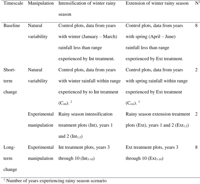
Table 1. Rainy season scenarios investigated in this study.
569
Timescale Manipulation Intensification of winter rainy season
Extension of winter rainy season N1
Baseline Natural
variability
Control plots, data from years with winter (January – March) rainfall less than range
experienced by Int treatment.
Control plots, data from years with spring (April – June) rainfall less than range experienced by Ext treatment.
8 Short-term change Natural variability
Control plots, data from years with winter rainfall within range experienced by to Int treatment (Cint). 2
Control plots, data from years with spring rainfall within range experienced by Ext treatment (Cext). 3
2
Experimental manipulation
Rainy season intensification treatment plots (Int), years 1 and 2 (Int1,2)
Rainy season extension treatment plots (Ext), years 1 and 2 (Ext1,2)
2 Long-term change Experimental manipulation
Int treatment plots, years 3 through 10 (Int3-10)
Ext treatment plots, years 3 through 10 (Ext3-10)
8
1 Number of years experiencing rainy season scenario 570 2 2004 and 2006 571 3 2003 and 2005 572 573 574 575 576 577 578 579 580
24
Figures
581
582 583
Figure 1. Change in (a) plant productivity and species richness, (b) consumer abundance and (c)
584
precipitation over the study period. For biotic response variables, mean values ± SE are shown for
585
each treatment in each year, with data from control plots shown by open circles, the Int treatment
586
shown by grey squares, and the Ext treatment shown by black triangles. Precipitation data are plotted
587
in a stacked graph, with winter (January – March) precipitation shown in black, spring (April to June)
588
precipitation shown in gray, and remaining precipitation in each year (October-December in the year
589
before sampling) shown in white.
590 591 592
25 593
Figure 2. Plant responses to intensification and extension of the annual rainy season.
594
Data represent mean + 1 s.e. for aboveground net primary production (a, b) and species richness (c, d)
595
under naturally and experimentally intensified (a, c) and extended (b, d) rainy seasons. In each panel,
596
the black line and grey shading show baseline conditions for that variable, as mean values + 1 s.e.
597
measured in control plots over the eight years of the study with typical seasonal rainfall levels. C(int) 598
and C(ext) denote measurements from control plots in years when seasonal rainfall levels were elevated 599
above long-term averages so that they were comparable with levels experienced in precipitation
600
addition treatments. Int(1,2) and Int(3-10) denote measurements from plots subjected to experimental 601
intensification of the rainy season via wintertime water addition in years 1 and 2 and years 3 through
602
10, respectively. Ext(1,2) and Ext(3-10) denote measurements from plots subjected to experimental 603
extension of the rainy season via springtime water addition in years 1 and 2 and years 3 through 10,
604
respectively. Different letters denote statistically significant differences (P < 0.05) between
605
treatments; treatments with the letter “a” are not significantly different from control plots in years
606
with typical seasonal rainfall levels.
607 608 609 610 611 612 613
26 614
Figure 3. Invertebrate responses to intensification and extension of the annual rainy season.
615
Data represent mean abundance + 1 s.e. for herbivores (a, b), predators (c, d), and parasitoids (e,f)
616
under naturally and experimentally intensified (a, c, e) and extended (b, d, f) rainy seasons. See
617
legend from Fig. 2 for explanation of symbols and terms.
618 619 620 621 622
27 623
Figure 4. Ecological relationships under ambient, intensified, and extended annual rainy seasons.
624
(a) Plant production versus plant species richness across years. (b) Consumer biomass versus plant
625
production across years. Control plots are represented by open circles, intensified rainy season (Int)
626
plots by grey squares, and extended rainy season (Ext) plots by black triangles.
627 628 629