User Guide Supply Chain Management

(1)

QAD Enterprise Applications 2008/2009

Standard Edition

User Guide

Supply Chain Management

Enterprise Operations Plan

Distribution Requirements Planning

Product Line Plan

Resource Plan

78-0730B QAD 2008/2009 Standard Edition June 2010

(2)

without the prior written consent of QAD Inc. The information contained in this document is subject to change without notice.

QAD Inc. provides this material as is and makes no warranty of any kind, expressed or implied, including, but not limited to, the implied warranties of merchantability and fitness for a particular purpose. QAD Inc. shall not be liable for errors contained herein or for incidental or consequential damages (including lost profits) in connection with the furnishing, performance, or use of this material whether based on warranty, contract, or other legal theory.

QAD and MFG/PRO are registered trademarks of QAD Inc. The QAD logo is a trademark of QAD Inc.

Designations used by other companies to distinguish their products are often claimed as trademarks. In this document, the product names appear in initial capital or all capital letters. Contact the appropriate companies for more information regarding trademarks and

registration.

QAD Inc.

100 Innovation Place

Santa Barbara, California 93108 Phone (805) 684-6614

Fax (805) 684-1890

(3)

About This Guide . . . 1

Chapter 1 Introduction to Supply Chain Management . . . 5

Enterprise Operations Plan (EOP) . . . 6

DRP and Other Planning Modules . . . 6

Electronic Data Interchange (EDI) . . . 7

Section 1 Enterprise Operations Plan . . . 9

Chapter 2 About Operations Plan . . . 11

Introduction to Operations Planning . . . 12

Operations Planning Example . . . 16

Module Overview . . . 18

Chapter 3 Required Implementation . . . 21

Introduction . . . 22

Setting Up Other Modules . . . 22

(4)

Manager Functions . . . 24

General Ledger . . . 24

Distribution Requirements Plan . . . 25

Items/Sites . . . 25

Resource Plan . . . 26

Work Orders . . . 26

Repetitive . . . 26

Material Requirements Plan . . . 27

Purchasing . . . 27

Setting Up the Operations Plan Module . . . 27

Review the General Ledger Calendar . . . 27

Build Calendar Cross-References . . . 28

Configure the Control Program . . . 29

Chapter 4 Family Data Implementation . . . 31

Defining Family Hierarchies . . . 32

Setting Up Hierarchies . . . 34

Copying Hierarchies . . . 35

Changing Subfamily Relationships . . . 36

Changing Subfamily Forecast Percentages . . . 37

Establishing Target Inventory Levels . . . 37

Setting Up Generic Coverage Factors . . . 39

Setting Up Date-Specific Coverage Factors . . . 40

Tracking Family Production Costs . . . 40

Chapter 5 End-Item Data Implementation . . . 43

Using Source Matrices . . . 44

Setting Up Source Matrices . . . 46

Using Line Allocations . . . 47

Setting Up Line Allocations . . . 48

Setting Target Inventory Levels . . . 49

(5)

Contents v

Setting Up Generic and Date-Specific Coverage Factors . . . 50

Tracking Pallet Data . . . 51

Setting Up Generic Pallet Information . . . 51

Setting Up Item Pallet Information . . . 52

Chapter 6 Data Collection . . . 53

Loading Data from Other Sites . . . 55

Loading Data from Non-QAD Databases . . . 59

Loading Item-Site Data . . . 59

Consolidating Loaded Data . . . 60

Maintaining Loaded Data . . . 60

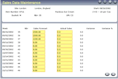
Changing Sales Data . . . 61

Reviewing Sales Data . . . 62

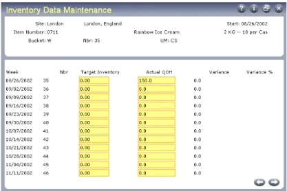
Changing Inventory Data . . . 62

Reviewing Inventory Data . . . 63

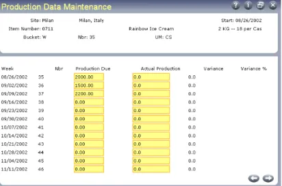
Changing Production Data . . . 64

Reviewing Production Data . . . 65

Chapter 7 Family-Level Planning . . . 67

Calculating Family Plans . . . 69

Maintaining Family Plans . . . 70

Changing Family Plans . . . 72

Reviewing Projected Profit . . . 75

Exploding Family Plans . . . 76

Reviewing Family Forecast Percentages . . . 76

Exploding Family Plans . . . 77

Rolling Up End-Item Changes . . . 78

Running Family Plan Rollup . . . 79

Chapter 8 End-Item Planning . . . 81

(6)

Running Source Matrix Explosion . . . 84

Maintaining Operations Plans . . . 86

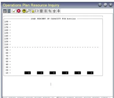
Reviewing Projected Resource Load . . . 86

Changing Site Operations Plans . . . 86

Reviewing Site Operations Plans . . . 88

Changing Line Operations Plans . . . 89

Reviewing Line Operations Plans . . . 90

Changing Line Schedules . . . 90

Reviewing Line Schedules . . . 97

Reviewing Projected Inventory Coverage . . . 97

Reviewing Site Utilization . . . 98

Reviewing Production Labor Hours . . . 98

Chapter 9 Transfer of Production Demands. . . 99

Exploding the Operations Plan into Orders . . . 100

Running Operations Plan Explosion . . . 101

Approving Orders to Other Modules . . . 103

Running Operations Plan Approval . . . 104

Running Operations Plan Batch Approval . . . 106

Balancing Target Inventory Levels and MRP . . . 106

Chapter 10 Performance Measurement. . . 109

Chapter 11 Simulation Planning . . . 113

Creating Simulation Plans . . . 114

Maintaining Simulation Plans . . . 116

Changing Site Simulation Plans . . . 116

Changing Line Simulation Plans . . . 117

Changing Simulation Line Schedules . . . 118

(7)

Contents vii

Chapter 12 System Administration . . . 121

Maintaining Static Data . . . 122

Deleting Old Data . . . 123

Recalculating Summary Records . . . 124

Chapter 13 Operations Plan Examples . . . 125

Family Plan Example . . . 126

Global Consolidation . . . 126

Family Plan Explosion . . . 130

Family Plan Rollup . . . 132

Operations Plan Example . . . 134

Source Matrix Explosion . . . 134

Section 2 DRP and Other Planning Modules . . . 141

Chapter 14 Distribution Requirements Planning . . . 143

DRP Functions . . . 144

DRP Life Cycle . . . 145

Purchase Orders and Sales Orders . . . 148

Setting Up DRP . . . 149

Purchase/Manufacture Code . . . 149

Source Networks . . . 150

Transportation Management . . . 151

Master Scheduling Distribution Items . . . 154

Set Up Control Programs . . . 155

Executing DRP . . . 155

DRP Modes . . . 155

DRP and MRP . . . 157

DRP Calculation and Processing . . . 158

(8)

MRP/DRP Calculations Using AppServer . . . 159

Synchronized MRP/DRP Calculations . . . 161

Managing Intersite Requests . . . 162

Intersite Requests at the Demand Site . . . 164

Intersite Requests at the Supply Site . . . 166

Managing Database Connections . . . 166

Using Distribution Orders . . . 167

Creating Distribution Orders . . . 168

Distribution Order Workbench . . . 174

Shipping Distribution Orders . . . 177

Using Distribution Order Processing . . . 180

Receiving Distribution Orders . . . 181

Reconciling Shipments . . . 182

DRP Action Messages . . . 183

Chapter 15 Product Line Plan . . . 187

Creating Product Line Plans . . . 188

Balancing Product Line Plans . . . 190

Maintaining Product Line Plans . . . 191

Chapter 16 Resource Plan . . . 193

Setting Up Resource Plans . . . 194

Resource Codes . . . 194

Resource Bills . . . 195

Calculating Resource Plans . . . 196

Evaluating Product Line Plans . . . 197

Evaluating Manufacturing Schedules . . . 197

(9)

About This Guide

Other QAD Documentation 2

Online Help 2 QAD Web Site 3 Conventions 4

(10)

This guide covers features related to Supply Chain Management in QAD 2008 Standard Edition.

Online Help

QAD provides an extensive online help system. Help is available for most fields found on a screen. Procedure help is available for most programs that update the database. Most inquiries, reports, and browses do not have procedure help.

(11)

About This Guide 3

For information on using the help system in the different environments, refer to User Guide: Introduction, User Guide: QAD Desktop, and User

Guide: QAD .NET User Interface.

QAD Web Site

QAD’s Web site provides a wide variety of information about the company and its products. You can access the Web site at:

http://www.qad.com

For users with a QAD Web account, product documentation is available for viewing or downloading from the QAD Online Support Center at:

http://support.qad.com/

You can register for a QAD Web account at the QAD Online Support Center. Your customer ID number is required. Access to certain areas is dependent on the type of agreement you have with QAD.

Most user documentation is available in two formats:

• Portable document format (PDF). PDF files can be downloaded from the QAD Web site to your computer. You can view them with the free Adobe Acrobat Reader.

• HTML. You can view user documentation through your Web browser. The documents include search tools for easily locating topics of interest.

(12)

Conventions

Several interfaces are available: the .NET User Interface, Desktop (Web browser), Windows, and character. To standardize presentation, the documentation uses the following conventions:

• Screen captures show the Desktop interface.

• References to keyboard commands are generic. For example, choose Go refers to:

• The Next button in .NET UI

• The forward arrow in Desktop

• F2 in the Windows interface

• F1 in the character interface

In the character and Windows interfaces, the Progress status line at the bottom of a program window lists the main UI-specific keyboard commands used in that program. In Desktop, alternate commands are listed in the right-click context menu. In the .NET UI, alternate commands are listed in the Actions menu.

For complete keyboard command summaries for each interface, refer to the appropriate chapters of User Guide: QAD .NET User Interface, User Guide: QAD Desktop, and User Guide: Introduction.

This document uses the text or typographic conventions listed in the following table.

If you see: It means:

monospaced text A command or file name. italicized

monospaced text

A variable name for a value you enter as part of an operating system command; for example, YourCDROMDir.

indented command line

A long command that you enter as one line, although it appears in the text as two lines.

Note Alerts the reader to exceptions or special conditions.

Important Alerts the reader to critical information.

Warning Used in situations where you can overwrite or corrupt data, unless you follow the instructions.

(13)

Chapter 1 Introduction to Supply

Chain Management

Enterprise Operations Plan (EOP) 6

DRP and Other Planning Modules 6 Electronic Data Interchange (EDI) 7

(14)

Fig. 1.1

Supply Chain Management

Enterprise Operations Plan (EOP)

¶See “Enterprise Operations Plan” on page 9.

Use Enterprise Operations Plan (EOP) to balance supply and demand and reduce inventory levels across the enterprise by consolidating data from multiple sites within domains in a single database and across multiple connected databases. The system determines whether database switching is needed based on the domain associated with the site in Site

Maintenance (1.1.13).

EOP helps planners establish global inventory and production levels to satisfy sales forecasts while meeting objectives for profitability, productivity, inventory and lead time reductions, and customer service.

DRP and Other Planning Modules

¶See “DRP and Other Planning Modules” on page 141.

Use Distributions Requirements Plan (DRP) to manage supply and demand between sites. DRP calculates item requirements at a site and generates DRP orders at the designated supply sites. DRP orders provide intersite demand to MRP at the supply site. DRP shipments manage the transfer of material between sites with appropriate inventory accounting and visibility of orders in transit.

To plan by product line rather than individual item, use Product Line Plan. You can plan shipments, production, inventory, backlogs, and gross margins—all measured by overall sales and cost to ensure that the plan meets all the financial needs of the business.

Supply Chain Management Enterprise Operations Plan (EOP) Distribution Requirements Plan (DRP)*

* and other planning modules

Electronic Data Interchange (EDI)

(15)

Introduction to Supply Chain Management 7

Use the Resource Plan to check resource loads for both the product line plan and the master schedule. Resource checking is a necessary step for validating the plans and master schedules before submitting them to MRP for detailed planning.

Electronic Data Interchange (EDI)

EDI is an important tool in supply chain management. You can use it to import and export standard business transactions between your company and its customers and suppliers using your e-mail system or network connections.

EDI eCommerce is a globally deployable EDI solution that provides EDI with reduced installation and support requirements. EDI eCommerce processes international EDI document standards with most major third-party EDI communications or translation software—referred to collectively as EC subsystems—currently on the market.

¶See User Guide: Release Management.

EDI is closely related to customer and supplier scheduled orders. Many EDI eCommerce programs can be used to import and export the documents that form the basis of scheduled order processing. For this reason, even though EDI is a supply chain function, it is not discussed in this volume. Rather, it is grouped together in the discussion of Release Management.

(16)

(17)

S

ECTION

1 Enterprise

Operations Plan

This section describes Enterprise Operations Plan:

About Operations Plan 11 Required Implementation 21 Family Data Implementation 31 End-Item Data Implementation 43 Data Collection 53

Family-Level Planning 67 End-Item Planning 81

Transfer of Production Demands 99 Performance Measurement 109 Simulation Planning 113 System Administration 121 Operations Plan Examples 125

(18)

(19)

Chapter 2 About Operations Plan

This chapter introduces general concepts associated with operations planning. Then, it describes how the Enterprise Operations Plan module works and how you use it.

Introduction to Operations Planning 12 Module Overview 18

(20)

Introduction to Operations Planning

Large manufacturing companies normally have multiple sites. Each site handles at least one of the following activities.

• Sales

• Inventory storage and distribution

• Production

Example A company has five sites, as shown in Figure 2.1. The headquarters is in London. Four additional sites are in Geneva, Paris, Dublin, and Milan.

Fig. 2.1

Example of Organization Structure

Within a site, it is relatively easy to balance sales forecasts, inventory, and capacity. However, it is much harder to do this between sites. For

example, Geneva often has inventory shortages, but Paris has surpluses. Also, Milan incurs high overtime costs even though Dublin has ample production capacity.

To control inventory levels and balance resources among sites, many manufacturers use supply chain management techniques such as:

• Setting up focused factories dedicated to specific manufacturing activities

• Consolidating purchasing across sites

• Defining target inventory coverage levels globally instead of by site These techniques help. But without a central production planning tool, balancing supply and demand between sites in the supply chain is still a difficult task. London Marketing Distribution London Marketing Distribution Geneva Marketing Distribution Geneva Marketing Distribution Paris Marketing Distribution Paris Marketing Distribution Dublin Manufacturing Dublin

Manufacturing ManufacturingMilan

Milan

Manufacturing

= Demand = Supply

(21)

About Operations Plan 13

Operations planning is a strategic and tactical production planning tool designed to do exactly this. It is especially useful in high-volume, make-to-stock companies.

As a strategic tool, you can use operations planning to:

• Project long-term labor, equipment, and cash needs.

• Develop long-term material procurement plans for negotiations with major suppliers.

As a tactical tool, you can use operations planning to:

• Optimize target inventory and production levels throughout the enterprise.

• Identify variances between planned and actual performance.

• Develop schedules for sites and production lines.

Enterprise resource planning (ERP) is an information system for planning the company-wide resources needed to take, make, ship, and account for customer orders. In companies that use ERP, operations planning is the key link between long-term business planning and medium- to short-term planning and execution activities (Figure 2.2).

Fig. 2.2

Operations Planning and ERP

(22)

Operations planning calculates target inventory levels that support company objectives for profitability, inventory and lead time reductions, customer service, and so on. It also calculates the corresponding

production demands. These demands eventually pass into production, purchasing, and material requirements planning (MRP).

The Enterprise Operations Plan module closely parallels the classic APICS model for sales and operations planning. However, it is superior in that it generates firm planned work orders that can replace master schedule orders. To prevent duplications, do not use the Forecast/Master Plan module for item-sites already included in operations planning. Figure 2.3 summarizes how operations planning transforms data.

Operations planning calculates target inventory levels based on upcoming sales forecasts. It also calculates production demands required for target inventory levels. For medium- to short-term planning, it nets these production demands against on-hand inventory balances.

Fig. 2.3

Operations Plan Data Flow

Operations planning transforms production demands into firm planned work orders, repetitive schedules, or purchase requisitions. It also passes these demands into MRP/DRP, which calculates the component

requirements. Operations Planning Operations Planning Work Orders Work Orders Repetitive Schedules Repetitive Schedules Purchase Requisitions Purchase Requisitions MRP/DRPMRP/DRP Sales Forecasts Sales

Forecasts InventoryBalances Inventory Balances

(23)

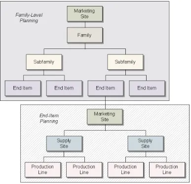
Operations planning includes two major planning levels:

• Family-level planning. High-volume, make-to-stock companies frequently have a wide variety of similar items that differ only by size, color, packaging, or other minor characteristic. To simplify long-term business planning, these companies forecast and plan production by product family.

• End-item planning. In the medium to short term, companies forecast and plan production for end items.

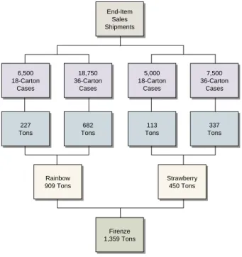
Figure 2.4 summarizes the relationships between the two levels.

Fig. 2.4

(24)

Operations Planning Example

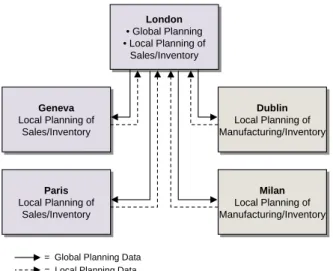
¶See Figure 2.1 on

page 12. Figure 2.5 shows the operations planning relationships between sites. In _{addition to marketing, London is the central site for operations planning.}

Each of the other four sites plans its own activities, then provides the local planning data to the London master scheduler.

Fig. 2.5

Planning Relationships

The London scheduler consolidates this data and calculates a weekly global operations plan for each product. This plan shows consolidated sales forecasts, target inventory levels, and production due.

London then distributes the global plan to all sites. The local site planners transform this plan into weekly production schedules.

In Table 2.1, London calculates a global operations plan. London, Geneva, and Paris generate sales forecasts. Milan and Dublin provide inventory required to satisfy these forecasts. London calculates global sales forecasts by consolidating its own forecasts with those from Geneva and Paris. Table 2.1 Global Sales Forecasts for London London • Global Planning • Local Planning of Sales/Inventory London • Global Planning • Local Planning of Sales/Inventory Geneva Local Planning of Sales/Inventory Geneva Local Planning of Sales/Inventory

= Global Planning Data = Local Planning Data

Paris Local Planning of Sales/Inventory Paris Local Planning of Sales/Inventory Dublin Local Planning of Manufacturing/Inventory Dublin Local Planning of Manufacturing/Inventory Milan Local Planning of Manufacturing/Inventory Milan Local Planning of Manufacturing/Inventory

Week Geneva Forecasts Paris Forecasts Global Forecasts

1 0 0 0

2 4,000 6,000 4,000 + 6,000 = 10,000

3 7,000 5,000 7,000 + 5,000 = 12,000

(25)

London calculates global target inventory levels to support the next two weeks of sales forecasts from London, Geneva, and Paris. Therefore, the target inventory level is the total global forecast for the next two weeks.

Table 2.2

Global Forecasts and Target Inventory Levels for London

Production due is the consolidated production requirement, calculated with the following formula.

(Sales Forecast + Target Inventory) – Previous Week’s Projected Quantity on Hand

For week 1, the projected quantity on hand is the ending inventory balance from the previous week (or 3,000, in this example). For weeks 2 to 9, projected quantity on hand equals the target inventory level for the previous week. Table 2.3 Production Calculations 5 4,500 4,500 4,500 + 4,500 = 9,000 6 5,000 5,000 5,000 + 5,000 = 10,000 7 6,000 5,000 6,000 + 5,000 = 11,000 8 6,000 6,000 6,000 + 6,000 = 12,000 9 8,000 5,000 8,000 + 5,000 = 13,000

Week Geneva Forecasts Paris Forecasts Global Forecasts

Week Global Forecasts Global Target Inventory Levels

1 0 10,000 + 12,000 = 22,000 2 10,000 12,000 + 11,000 = 23,000 3 12,000 11,000 + 9,000 = 20,000 4 11,000 9,000 + 10,000 = 19,000 5 9,000 10,000 + 11,000 = 21,000 6 10,000 11,000 + 12,000 = 23,000 7 11,000 12,000 + 13,000 = 25,000 8 12,000 13,000 + 0 = 13,000 9 13,000 0

Wk Forecasts Target Inv Prev QOH Global Production Due

1 0 22,000 3,000 (0 + 22,000) – 3,000 = 19,000

2 10,000 23,000 22,000 (10,000 + 23,000) – 22,000 = 11,000 3 12,000 20,000 23,000 (12,000 + 20,000) – 23,000 = 9,000 4 11,000 19,000 20,000 (11,000 + 19,000) – 20,000 = 10,000

(26)

London will use the operations plan to view the global picture of sales forecasts, target inventory, and production due for this item. Milan and Dublin will use it for site-level planning, scheduling, and manufacturing activities. Table 2.4 Production Calculations and Projected Quantities on Hand

Module Overview

The Enterprise Operations Plan module has many useful features:

• Planning at family and/or end-item levels

• Demand consolidation from multiple sites in multiple domains, both within a single database and across multiple databases

• Production demands based on sales forecasts and inventory balances

• Target inventory levels in weeks of coverage, by effective date

• Intersite supply and demand relationships by effective date

• Production demands allocated to sites and lines by percentage

• Interface with resource planning

5 9,000 21,000 19,000 (9,000 + 21,000) – 19,000 = 11,000 6 10,000 23,000 21,000 (10,000 + 23,000) – 21,000 = 12,000 7 11,000 25,000 23,000 (11,000 + 25,000) – 23,000 = 13,000 8 12,000 13,000 25,000 (12,000 + 13,000) – 25,000 = 0

9 13,000 0 13,000 (13,000 + 0) – 13,000 = 0

Wk Forecasts Target Inv Prev QOH Global Production Due

Wk Forecasts Target Inventory Production Due Projected QOH

1 0 22,000 19,000 22,000 2 10,000 23,000 11,000 23,000 3 12,000 20,000 9,000 20,000 4 11,000 19,000 10,000 19,000 5 9,000 21,000 11,000 21,000 6 10,000 23,000 12,000 23,000 7 11,000 25,000 13,000 25,000 8 12,000 13,000 0 13,000 9 13,000 0 0 0

(27)

• Production line scheduling

• Production demand transfer to other modules

• Performance measurement reporting

• Simulation planning

Figure 2.6 summarizes the module work flow.

Fig. 2.6

Operations Plan Work Flow

To generate any plan or performance measurement report, you must first collect item sales, inventory, and production data from company sites. Operations planning activities do not affect the source transactions, only the collected data.

Family-level planning is optional but useful for limiting the number of items to be planned and for grouping items by brand name, target market, production process, and so on. To develop the family plan, you first generate site sales forecasts for each family item. Then, you consolidate these forecasts and calculate the family plan.

You verify the production quantities against known capacity constraints and modify them if necessary. To experiment with planning scenarios, create simulation plans. Then, you explode the plan to calculate the corresponding dependent end-item demand. This step passes the family plan production requirements into the end-item planning cycle.

= optional

Collect transaction data. Collect transaction data.

Measure performance. Measure performance.

Develop family plan. Develop family plan.

Develop operations plan. Develop operations plan.

Transfer production demands. Transfer production demands.

(28)

Operations planning continues at the end-item level, and the processing steps roughly parallel those at the family level. To develop the end-item operations plan, you first load and consolidate sales forecast and

inventory data for all company sites. Then, you use this data to calculate the operations plan for each end item.

You verify the production quantities against known capacity constraints and modify them if necessary. Again, you can create simulation plans. If you plan at the family level, you must also roll the changes back into the family plan.

Production demands from the operations plan affect subsequent

manufacturing, planning, and purchasing activities. Once you are satisfied with the operations plan, run an explosion process to generate firm planned orders. These orders are similar to master schedule orders generated by the Forecast/Master Plan module. You can approve these orders as firm planned work orders, repetitive schedules, or purchase requisitions.

¶See User Guide: Manufacturing

for information on MRP.

To ensure that MRP and sales forecast records remain synchronized, also run a balancing utility. Finally, run MRP/DRP to generate planned orders for component requirements.

At the end of the planning cycle, you measure actual vs planned sales, inventory, and production performance. To do this, load end-item data using the same data collection programs used to load plan data. If you plan at the family level, you also roll the actual end-item performance back up to the family level. Then, print and review performance reports.

(29)

Chapter 3 Required

Implementation

This chapter describes setup activities required to use operations planning.

Introduction 22

Setting Up Other Modules 22

(30)

Introduction

Regardless of how you plan to use the Enterprise Operations Plan module, it is important to set up data correctly not only in the module itself, but in all other modules that interact with it.

Table 3.1

Modules and Operations Plan

You also must perform some setup tasks within the Enterprise Operations Plan module.

Setting Up Other Modules

Figure 3.1 shows the modules that interact with operations planning calculations. Both the family plan and operations plan incorporate sales forecasts and inventory balances. The operations plan, in turn, can generate MRP and DRP requirements, work orders, repetitive schedules, and purchase requisitions.

Module Data

Multiple Domains and Database Domain and database connections

Manager Functions Holidays, shop calendar, generalized codes, security

General Ledger Financial calendar

Distribution Requirements Plan Control, network codes, source networks

Items/Sites Sites and site security, product lines, unit of measure conversions, items

Resource Plan Resource bills, item resource bills

Work Orders Control

Repetitive Production lines, shift calendars Material Requirements Plan Control

(31)

Required Implementation 23

Fig. 3.1

Plan Calculation Inputs/Outputs

Figure 3.2 shows the modules that provide data to operations planning performance reports. Performance reports include quantities from completed work orders and repetitive schedules, purchase order receipts, sales order shipments, and inventory balances.

Fig. 3.2

Performance Measurement Inputs

You should implement most or all of the other required modules before implementing Operations Plan.

Implementation is also a good time to review your company’s coding schemes and other business practices to take advantage of capabilities offered by the system.

Family Plans and Operations Plans Inventory Control Distribution Requirements Plan Forecast/

Master Plan Repetitive

Material Requirements Plan Purchasing Work Orders

Family and End-Item Performance Measurement Purchasing Repetitive Work Orders Sales Orders/ Invoices Inventory Control

(32)

Multiple Database

¶See User Guide: Manager Functions.

If you plan to import operations planning data from sites in other domains within a single database or in separate databases, you must ensure that you use consistent codes for items, sites, and so on. Inconsistencies can create problems transferring planning data.

If the domains are in different databases, ensure that database connection information is properly set up. The system determines when database switching is needed automatically based on the domain associated with the site in Site Maintenance (1.1.13).

If a database runs other manufacturing software, make sure that the codes from that database are duplicated in the database used for operations planning.

Manager Functions

¶See User Guide: Manager Functions for information on calendars, generalized codes, and security.

Operations Plan uses the holiday calendar if Move Holiday Production Backward is Yes in Operations Plan Control (33.1.24). In this case, calculations reschedule production backward for non-production weeks. Generalized codes for item type (pt_part_type) and item group (pt_group) are selection criteria in many operations planning reports and processes. Set up security for most operations planning programs to prevent unauthorized changes to master data, family plans, and operations plans. This also reduces the possibility that someone will prematurely copy simulation plans over the live plans, approve operations plan orders, or delete records. You can set up security at the menu and field levels.

General Ledger

¶See User Guide: Financials A.

Operations planning inquiries and reports use the company financial calendar to display the family plan and operations plan in financial periods as well as calendar weeks. Before you implement Operations Plan, set up financial calendars to support the entire operations planning horizon.

(33)

Distribution Requirements Plan

¶See Chapter 14, “Distribution Requirements Planning,” on page 143.

In multisite environments, use the Distribution Requirements Plan module to link sales forecasts and their corresponding production requirements.

Set DRP Control (12.13.24) to support combined MRP/DRP processing. That way, whenever you run MRP, the system also runs DRP, and vice versa. DRP uses the network and source network codes to distribute operations plan item requirements among company sites.

Items/Sites

¶See User Guide: Manager Functions.

Most operations planning records and activities are associated with specific company sites. Set up site security in the System Security menu (36.3).

All items used for operations planning are associated with a product line. Product line is a selection criteria in some operations planning reports and processes.

Set up unit of measure conversion factors whenever you plan sales, inventory, and production in different units of measure. For example, you may plan sales and inventory in cases, but production in tons. Similarly, you need conversion factors whenever you use different units of measure for family-level and end-item planning. You may plan in metric tons at the family level but use kilos at the end-item level.

Set up item and item-site records for all items included in operations planning calculations.

• End items are grouped for family-level planning under a family item number.

• The operations plan approval programs use the item-site Purchase/ Manufacture code. Set it to blank or M for manufactured items, L for line manufactured items, W for flow items, P for purchased items, or F for family and subfamily items. For DRP items, set it to D in item-site records for marketing item-sites—item-sites that generate sales forecasts for the item.

(34)

• Operations planning uses the time fence. When you calculate or explode the operations plan, you can protect items from last-minute changes inside the time fence.

• For purchased items, operations planning uses inspection, safety, and purchasing lead times for production scheduling.

• For manufactured items, operations planning uses manufacturing and safety lead times for production scheduling.

• Operations planning target inventory calculations ignore safety stock quantities.

Resource Plan

¶See Chapter 16, “Resource Plan,” on page 193.

A primary objective of operations planning is to verify projected production load from the family plan and operations plan against available capacity. Therefore, you must set up resource bill records for critical resources such as equipment and labor. Operations planning uses item resource bills to calculate projected load for individual items.

Work Orders

¶See User Guide:

Manufacturing. To process operations plan production requirements as work orders, _{implement the Work Orders module.}

Repetitive

¶See User Guide: Manufacturing.

To process operations plan production requirements as repetitive schedules, implement the Repetitive module.

In the Enterprise Operations Plan module, you can allocate production requirements by percentage between multiple lines in a site. The production line record has an additional Primary Line field when you implement Operations Plan. This field identifies whether a line is an item’s sole production line. If your company currently uses Repetitive, during the conversion process, you must run Production Line Update (33.25.3) to update existing production line records before you can set up line allocation records in Operations Plan. Operations Plan also uses the line’s run crew size to project site labor hours.

(35)

Operations Plan uses line shift calendars to calculate the number of available production hours and utilization for each production line. If no shift calendar is available, it uses the shop calendar for the supply site.

Material Requirements Plan

¶See User Guide: Manufacturing.

If you use DRP, you can set MRP Control (23.24) to support combined MRP/DRP processing. That way, when you run MRP, the system also runs DRP, and vice versa.

Purchasing

¶See User Guide: Distribution A.

To process operations plan production requirements as purchase requisitions, implement the Purchasing module.

Setting Up the Operations Plan Module

Programs used for Operations Plan system setup are located in the System Setup Menu (33.1). The system setup is mandatory for all installations.

• Review the GL calendar.

• Build calendar cross-references.

• Set up Operations Plan Control.

Review the General Ledger Calendar

Before building calendar cross-references, review the general ledger calendar.

• Use GL Calendar Browse (33.1.1) to show calendar periods starting with a specific fiscal year.

• Use GL Calendar Report (33.1.2) to show calendar periods for a range of entities and fiscal years.

Note The system defines the first week of a new calendar year as the first Thursday in January, in accordance with ISO standards.

(36)

Build Calendar Cross-References

In the Enterprise Operations Plan module, you can plan production either in calendar weeks (Monday–Sunday) or in financial periods. Calendar Cross-Reference Build (33.1.4) creates records that link the calendar and the financial calendar.

Fig. 3.3

Calendar Cross-Reference Build (33.1.4)

Year/To. Enter a range of calendar years, starting with the current year.

Table 3.2 shows typical linkages created by the build process.

Table 3.2

Calendar Cross-References

If a calendar week spans two financial periods, the build assigns the week to the period associated with the Monday date.

Example You run the build and you have a monthly financial calendar. Week 005 is January 29 – February 4, but the week is linked to period 1 because Monday, January 29 is still in period 1. The build does this because planning activities assign item quantities to the Monday of the week.

Use Calendar Cross-Reference Inquiry (33.1.5) to verify that cross-references between calendar weeks and general ledger periods now exist for all years in the planning horizon, including the current year. Before planning for a new year, verify that cross-references exist for that year. If they do not, build them.

Shop Calendar Weeks Fiscal Periods

001 January 1 – 7 = 001 January 1 – 31 002 January 8– 14 = 001 January 1 – 31 003 January 15 – 21 = 001 January 1 – 31 004 January 22– 28 = 001 January 1 – 31 005 January 29 – February 4 = 001 January 1 – 31 006 February 5 – 11 = 002 February 1 – 29

(37)

Configure the Control Program

The settings in Operations Plan Control (33.1.24) affect family plan and operations plan calculations. You can reconfigure the Control at any time. Changes to Control settings affect only subsequent planning activities.

Fig. 3.4

Operations Plan Control (33.1.24)

Use Operations Plan. Enter Yes to activate operations planning fields in other modules.

Maximum Weeks Coverage. Enter the maximum number of upcoming weeks (greater than zero but less than 99.99) the system should scan when netting sales forecasts against inventory balances. This setting affects the processing time of these calculations.

Move Holiday Production Backward. Enter Yes to prevent the system from scheduling production for production weeks. A non-production week is one that has no scheduled work days. Every day in the non-production week must be set up as a holiday in Holiday Maintenance (36.2.1).

Use Rounding. Enter Yes if family plan and operations plan

calculations should round item quantities to whole numbers. Enter No if they should calculate decimal quantities.

(38)

(39)

Chapter 4 Family Data

Implementation

Before you implement data for family-level operations planning, you must implement the standard system data and Enterprise Operations Plan module data listed in Chapter 3.

Introduction 32

Defining Family Hierarchies 32

Establishing Target Inventory Levels 37 Tracking Family Production Costs 40

(40)

Introduction

Companies typically do family-level operations planning in the long- to medium-term horizon, anywhere from six months to three years. They use it to:

• Project long-term labor, equipment, and financial commitments.

• Develop long-term material procurement plans for negotiations with strategic suppliers.

For family-level planning, the system uses three sets of data elements, as shown in Figure 4.1. You can set them up in any order.

Fig. 4.1

Family Data Implementation Work Flow

Programs used for family data implementation are located in the Family Setup Menu (33.3) and in the Item Setup Menu (33.5).

Defining Family Hierarchies

For operations planning, the family hierarchy defines several things:

• Nature of demand relationships for a product family

• End items and subfamilies in the family, and the percentage of total family sales forecast contributed by each

• Marketing sites that generate sales forecasts

Family hierarchies resemble product structures. The hierarchy consists of a parent family item and one or more subfamilies. Subfamilies can be either lower-level hierarchies or end items. Subfamilies in the lowest level must be end items. Within a hierarchy, each subfamily contributes a percentage of the total sales forecast for the family item.

= optional

Set up family hierarchies. Set up family hierarchies.

Set up family target inventory levels.

Set up family production costs. Set up family production costs.

(41)

Family Data Implementation 33

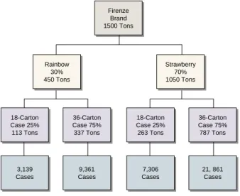
Example The Firenze brand is a top-level family with its marketing site in London. The Firenze family has two subfamilies, Rainbow flavor (30% of demand) and Strawberry flavor (70% of demand). Each subfamily is also a lower-level hierarchy with two end items, an 18-carton case and a 36-carton case.

Fig. 4.2

Family Hierarchies

You can set up flexible hierarchies that mirror your company’s planning groups. For example, you can set up hierarchies by buyer/planner group, brand, flavor, color, distribution channel, sales region, production line, and so on. The same subfamily or end item can belong to multiple families. Marketing may plan items by geographic region or brand name, but production plans by similarity of manufacturing process.

Subfamily relationships and percentages usually vary by marketing site and planning year. Typically, you set up multiple sets of subfamily relationships for each family hierarchy. Figure 4.3 summarizes the setup work flow. Firenze Brand Firenze Brand Rainbow Rainbow 18-Carton Case 25% 18-Carton Case 25% 36-Carton Case 75% 36-Carton Case 75% Strawberry Strawberry 18-Carton Case 25% 18-Carton Case 25% 36-Carton Case 75% 36-Carton Case 75% Rainbow 30% Rainbow 30% Strawberry70% Strawberry 70%

(42)

Fig. 4.3

Hierarchy Setup Work Flow

Setting Up Hierarchies

To set up new hierarchies and to change forecast percentages for existing hierarchies, use Family Hierarchy Maintenance (33.3.1). When you set up hierarchies, the system checks for cyclical relationships to prevent you from accidentally assigning a subfamily to itself.

Set up a hierarchy for every family item. Start from the lowest level and work upward to the top family level. The subfamilies for the lowest level must be end items.

Fig. 4.4

Family Hierarchy Maintenance (33.3.1)

Family Item. Enter the family item number. This item must be set up previously in Item Master Maintenance with a Purchase/Manufacture code of F (family).

Subfamily Item. Enter the end-item or family-item number to assign to this level of the hierarchy.

Site. Enter the site code.

Effective Year. Enter the hierarchy year.

Set up generic hierarchies. Set up generic hierarchies.

Copy for marketing sites. Copy for marketing sites.

Adjust for specific sites. Adjust for specific sites.

Copy for planning years. Copy for planning years.

Adjust for specific sites. Adjust for specific sites.

(43)

Forecast Percent. Enter the percentage of the total family sales forecast typically contributed by this subfamily. Family Plan Explosion (33.7.14) can use this percent to calculate dependent end-item production demands from family demands.

Remarks. Optionally enter a remark about the subfamily level. This remark prints on the Family Hierarchy Report (33.3.3).

Use three programs to review hierarchy data:

• Family Hierarchy Inquiry (33.3.2) displays subfamily levels in a family hierarchy by year, site, level, and item.

• Family Hierarchy Report (33.3.3) is similar, but you can select information for a range of items, sites, and years.

• Family Hierarchy Where-Used Inquiry (33.3.8) displays family items that include the specified subfamily.

Copying Hierarchies

To copy hierarchy records, use Family Hierarchy Copy (33.3.5). For every family item, you must set up subfamily relationships for all marketing sites and years in the planning horizon.

Fig. 4.5

Family Hierarchy Copy (33.3.5)

Source Family Item. Enter the family item number for the source subfamily.

Source Site. Enter the code for the source subfamily’s marketing site.

Effective Year. Enter the effective year for the source subfamily relationship.

(44)

Target Family Item. Enter the family item number for the target subfamily.

Target Site. Enter the code for the target subfamily’s marketing site.

Effective Year. Enter the hierarchy year for the target subfamily relationship.

Changing Subfamily Relationships

After you copy hierarchies, use Family Hierarchy Change (33.3.6) to add, delete, or replace subfamilies for individual marketing sites and years.

Note Regardless of how you change subfamilies, you must later adjust the forecast percentages for all other subfamilies at the affected level, in all hierarchy records you change.

Fig. 4.6

Family Hierarchy Change (33.3.6)

Subfamily Item. Enter the number of an end item or family item for the subfamily level affected by the change.

Site/To. Enter a range of sites to be updated.

Effective Year/To. Enter a range of years to be updated.

Action. Enter the action you want to take with this family relationship:

• Add. The system adds it (along with its lower-level subfamilies, if any) to the same level of the hierarchy as the subfamily item you specify. It also copies the existing subfamily’s forecast percent to the new subfamily.

(45)

• Delete. The system deletes the subfamily relationship with any higher- or lower-level hierarchies. However, it does not delete lower-level hierarchies previously linked to the subfamily.

• Replace. The system replaces only the subfamily item. It does not change lower-level subfamily relationships.

New Subfamily Item. Enter the number of the family item or end item to replace the specified subfamily item.

UM. The screen displays the inventory unit of measure from the item master record.

Changing Subfamily Forecast Percentages

Whenever you adjust subfamily relationships, you must also adjust forecast percentages for other subfamilies at the affected level. For each level, make sure the percentages add up to 100%.

Fig. 4.7

Family Hierarchy Maintenance (33.3.1)

Establishing Target Inventory Levels

Operations planning calculates global target inventory levels to support an item’s sales forecasts. In turn, it calculates production requirements based on target inventory levels.

If you do not specify otherwise, the system automatically sets each week’s target inventory level to zero. When set this way, you cannot build up inventory for future demands. You also cannot anticipate inventory shortages or surpluses.

Subfamily Forecast Percent

(46)

To establish target inventory levels, define global weeks-of-coverage factors for minimum, average, and maximum target inventory levels. This method requires more implementation effort. However, it does support inventory buildup for upcoming sales forecasts.

Table 4.1 illustrates how the system uses coverage factors on the family plan. In the example, the system uses an average cover factor of 2.0 to calculate the target inventory level.

Table 4.1

Weeks of Coverage on Operations Plan

When you change production due quantities on the plan, it uses the minimum (–) and maximum (+) factors to alert you to potential inventory shortages and surpluses relative to the average coverage level. This is illustrated in Table 4.2, which assumes a minimum coverage of 1.0 and a maximum of 3.0. Table 4.2 Weeks of Coverage on Operations Plan—Production Due Quantities Changed

Note You can define coverage factors for either top-level family items or for end items. However, to prevent the system from inflating inventory, do not set up coverage factors for both levels or for intermediate subfamily levels. No. Sales Forecast Target Inventory Production Due Projected QOH Coverage 1 0 500 500 500 2.0 2 300 700 500 700 2.0 3 200 500 0 500 1.0 4 500 0 0 0 0.0 No. Sales Forecast Target Inventory Production Due Projected QOH Coverage 1 0 500 200 200 0.7 – 2 300 700 500 400 1.4 3 200 500 0 200 0.4 – 4 500 0 0 –300 0.0 –

(47)

Setting Up Generic Coverage Factors

Use Weeks of Coverage Maintenance (33.5.1) to set up an item’s generic coverage factors. Coverage factors are global, not site-specific, and they must be positive whole numbers.

Fig. 4.8

Weeks of Coverage Maintenance (33.5.1)

Item Number. Enter the family item number.

Minimum Weeks of Coverage. Enter the minimum number of weeks of global inventory coverage required for this item. The system uses this factor to calculate and display projected inventory shortages.

Average Weeks of Coverage. Enter the number of weeks of

upcoming sales forecasts that corresponds to your company’s desired inventory coverage level for this item. Plan calculations use this factor to calculate target inventory levels.

Maximum Weeks of Coverage. Enter the maximum number of weeks of global inventory coverage required for this item. The system uses this factor to calculate and display projected inventory surpluses. Use two programs to review weeks of coverage factor data:

• Weeks of Coverage Inquiry (33.5.2) displays coverage factors by item, purchase/manufacture code, and buyer/planner.

• Weeks of Coverage Report (33.5.3) is similar to the inquiry, but you can also select information for a range of items.

(48)

Setting Up Date-Specific Coverage Factors

To manage items with varying coverage levels, set up date-specific factors in Coverage by Date Maintenance (33.5.5). You must set up generic coverage factors before date-specific factors.

Fig. 4.9

Coverage by Date Maintenance (33.5.5)

¶See page 39. This program is similar to Weeks of Coverage Maintenance (33.5.1) but has two additional fields.

Start. Enter the start date for using this record in operations planning. The default is the system date.

End. Enter the end date for using this record in operations planning, or leave it blank.

Use two programs to review date of coverage factor data:

• Coverage by Date Inquiry (33.5.6) displays coverage factors by item, and purchase/manufacture code.

• Coverage by Date Report (33.5.7) enables you to select information for a range of items and start/end dates.

Tracking Family Production Costs

You can record reference information on production costs for product families. However, Operations Plan does not use this information in family plan calculations.

You can maintain multiple sets of hourly production costs for each family item. Each set of costs is uniquely identified by the cost set code and the family item site. If your company uses the Cost Management module, you can set up family costs for a variety of cost sets.

(49)

Use Family Item Cost Maintenance (33.3.13) to set up family item production costs.

Fig. 4.10

Family Item Cost Maintenance (33.3.13)

Family Item. Enter the family item number.

Cost Set. Enter the cost set code.

Cost Set Type. The screen displays the cost set type for the cost set.

Costing Method. The screen displays the costing method for the cost set.

Production Rate. Enter the average hourly production rate for end items in this family. The production rate is the number of units of the family item that can normally be produced per hour on a production line.

Cost. Enter the average hourly production cost for end items in this family. The production cost is the normal hourly production cost for the specified number of units of the family item.

(50)

Use two programs to review family item cost data:

• Family Item Cost Inquiry (33.3.14) displays production rates and costs by family item, site, and cost set.

• Family Item Cost Report (33.3.15) enables you to select information for a range of items, sites, and cost sets.

(51)

Chapter 5 End-Item Data

Implementation

Before you implement data for end-item operations planning, you must implement the standard data and Enterprise Operations Plan module data listed in Chapter 3.

Introduction 44

Using Source Matrices 44 Using Line Allocations 47

Setting Target Inventory Levels 49 Tracking Pallet Data 51

(52)

Introduction

Companies typically do end-item operations planning in a short to medium-term time frame, usually less than six months. They use it to:

• Optimize target inventory and production levels throughout the enterprise.

• Develop production schedules for supply sites and production lines.

• Identify variances between planned and actual performance. For end-item planning, the system uses four sets of data elements, as shown in Figure 5.1. You can set them up in any order.

Fig. 5.1

End-Item Data Implementation Work Flow

Using Source Matrices

For operations planning, the item source matrix defines the nature of supply and demand relationships for end items. It identifies the marketing sites that generate sales forecasts. It also defines how the operations plan calculation distributes global production demands to supply sites.

¶See “Source Networks” on page 150.

Item source matrices resemble single-level DRP source networks. The source matrix consists of one or more marketing sites. Each marketing site, in turn, has one or more supply sites. Each supply site has a percentage that specifies how much of the item’s global production demand it contributes.

Set up source matrices. Set up source matrices.

Set up production line allocations. Set up production line allocations.

Set up target inventory levels. Set up target inventory levels.

Set up pallets. Set up pallets.

(53)

End-Item Data Implementation 45

Figure 5.2 shows a sample source matrix.

Fig. 5.2

Sample Source Matrix

The source matrix for item 0711 has three marketing sites that generate sales forecasts—London, Geneva, and Paris. London has two supply sites—Dublin, which supplies 50% of London’s production demand, and Milan, which supplies 50%. Geneva and Paris each have one supply site, Milan, which supplies 100% of their production demands.

¶See “Managing Intersite Requests” on page 162.

Note For better tracking of requirements between sites, multisite companies should use Operations Plan together with DRP. DRP generates intersite requests that identify the marketing sites that originated the demands.

To include an item in the operations plan, you must set up a source matrix for it. The same site can be both a marketing site and a supply site (set supply percent to 100%).

If you use DRP, the operations planning source matrix relationships for marketing and supply sites must mirror the DRP source networks.

Source Matrix Item 0711 Source Matrix Item 0711 London

London GenevaGeneva

Dublin 50% Dublin 50% Milan 50% Milan 50% Paris Paris Milan 100% Milan 100%

(54)

Setting Up Source Matrices

To set up source matrices, use Source Matrix Maintenance (33.5.13).

Fig. 5.3

Source Matrix Maintenance (33.5.13)

Item Number. Enter the end-item number.

Marketing Site. Enter the code for the marketing site. A marketing site is any site that generates sales forecasts. Examples include sales offices and distribution centers. An item can have multiple marketing sites in its source matrix.

Supply Site. Enter the code for the supply site. A supply site is any site that provides inventory to a marketing site. For manufactured items, the factory is typically the supply site. For purchased items, the purchasing site is the supply site. In a source matrix, a marketing site can have multiple supply sites.

Start. Enter the start date for using this source matrix in operations planning. To use the source matrix to calculate this week’s operations plan, you must set the start date to the previous Monday or earlier.

End. Enter the end date for using this record in operations planning, or leave it blank.

Supply Percent. Enter the percentage of the marketing site’s

production requirement provided by this supply site. If the marketing site and supply site are the same, enter 100.0%. The system does not verify that the percentages for a marketing site’s supply sites total 100.0%.

Transport Code. Enter the transportation code (if any) for inventory the supply site provides to the marketing site. Record this if needed for reference.

(55)

Lead Time. Enter the transportation lead time (if any) for inventory the supply site provides to the marketing site. Record this if needed for reference.

Use two programs to view source matrix data:

• Source Matrix Inquiry (33.5.14) shows marketing and supply site relationships by item.

• Source Matrix Report (33.5.15) is similar, but you can specify ranges of items, sites, and effectivity dates.

Using Line Allocations

Within a supply site, items can be produced on one or more production lines. The line allocation defines how production is distributed between these lines. Figure 5.4 shows how the Milan supply site allocates 25% of its production demand to Line 1 and the remaining 75% to Line 2.

Fig. 5.4 Production Line Allocations Source Matrix Item 0711 Source Matrix Item 0711 London

London GenevaGeneva

Dublin 50% Dublin 50% Milan50% Milan 50% Paris Paris Milan 100% Milan 100% Line 001 25% Line 001 25% Line 002_75% Line 002 75%

(56)

Setting Up Line Allocations

To set up production line allocations, use Line Allocation Maintenance (33.5.17). Set up line allocations only for items produced on multiple production lines within a site. The line percentages must total 100%.

Fig. 5.5

Line Allocation Maintenance (33.5.17)

Item Number. Enter the end-item number.

Production Line. Enter the code for the item’s production line at this site.

Description. The system displays the production line description from Production Line Maintenance (18.1.1).

Percent. Enter the production line allocation percentage. When you press Go, the system verifies that the total line percentage is 100%. Use Line Allocation Inquiry (33.5.18) to view line allocations by site and item number.

(57)

Setting Target Inventory Levels

Operations planning calculates global target inventory levels to support an item’s sales forecasts. In turn, it calculates production requirements based on target inventory levels.

If you do not specify otherwise, the system automatically sets each week’s target inventory level to zero. In this case, you cannot build up inventory for future demands. You also cannot anticipate inventory shortages or surpluses.

There are three methods to establish global target inventory levels for end items:

• Calculate target inventory levels based on production demands exploded from the family plan. This is an easy method for items initially planned at the family level. No additional setup is required.

• Calculate target inventory levels based on manually recorded

quantities. This method is precise. However, it is hard to maintain this information for many items because it changes constantly. Also, it offers no visibility to project shortages and surpluses.

• Calculate target inventory levels based on upcoming sales forecasts (weeks of coverage). For this method, you define global weeks-of-coverage factors for minimum, average, and maximum target inventory levels. This method requires more implementation effort. However, it does support inventory buildup for upcoming sales forecasts.

Note You can define coverage factors for either top-level family items or end items. However, to prevent the system from inflating inventory, do not set up coverage factors for both levels or for intermediate subfamily levels.

Table 5.1 illustrates how the system uses coverage factors on the operations plan. In the example, the system uses an average coverage factor of 2.0 to calculate the target inventory level.

Table 5.1 Weeks of Coverage on Operations Plan No. Sales Forecast Target Inventory Production Due Projected QOH Coverage 1 0 500 500 500 2.0 2 300 700 500 700 2.0

(58)

When you change production due quantities on the plan, it uses the minimum (–) and maximum (+) factors to alert you to potential inventory shortages and surpluses relative to the average coverage level. This is illustrated in Table 5.2, which assumes a minimum coverage of 1.0 and a maximum of 3.0. Table 5.2 Weeks of Coverage on Operations Plan—Production Due Quantities Changed

Loading Target Inventory Quantities

¶See Chapter 6, “Data

Collection,” on page 53.

There are two ways to load target inventory quantities manually:

• If you have already recorded target inventory quantities in a non-QAD database, use Site Data Maintenance (33.13.3) and Item-Site Data Consolidation (33.13.6) to load them.

• Manually record quantities using Inventory Data Maintenance (33.13.17).

Setting Up Generic and Date-Specific Coverage Factors

¶See “Setting Up Generic Coverage Factors” on page 39 and “Setting Up Date-Specific Coverage Factors” on page 40.

To set up generic and date-specific coverage factors for end-items, use the same programs described for setting up families. In the Item Number field, enter the end-item number. Coverage factors must be positive numbers. They can be either whole numbers or decimals.

3 200 500 0 500 1.0 4 500 0 0 0 0.0 No. Sales Forecast Target Inventory Production Due Projected QOH Coverage No. Sales Forecast Target Inventory Production Due Projected QOH Coverage 1 0 500 200 200 0.7 – 2 300 700 500 400 1.4 3 200 500 0 200 0.4 – 4 500 0 0 –300 0.0 –