Extended gcd algorithms
George Havas
∗B.S. Majewski
†K.R. Matthews
‡Abstract
Extended gcd calculation has a long history and plays an impor-tant role in computational number theory and linear algebra. Recent results have shown that finding optimal multipliers in extended gcd calculations is difficult. We study algorithms for finding good mul-tipliers and present new algorithms with improved performance. We present a well-performing algorithm which is based on lattice basis reduction methods and may be formally analyzed. We also give a relatively fast algorithm with moderate performance.
1
Introduction
Euclid’s algorithm for computing the greatest common divisor of 2 numbers is considered to be the oldest proper algorithm known ([12]). This algorithm can be amplified naturally in various ways. Thus, we can use it recursively to compute the gcd of more than two numbers. Also, we can do a constructive computation, the so-called extended gcd, which expresses the gcd as a linear combination of the input numbers.
Extended gcd computation is of particular interest in number theory (see [4, chapters 2 and 3]) and in computational linear algebra ([8, 9, 11]), in
∗Key Centre for Software Technology, Department of Computer Science, University of
Queensland, Queensland 4072, Australia,email: [email protected]
†Key Centre for Software Technology, Department of Computer Science, University of
Queensland, Queensland 4072, Australia,email: [email protected]
‡Queensland Centre for Number Theory and Exact Matrix Computation,
Depart-ment of Mathematics, University of Queensland, Queensland 4072, Australia, email: [email protected]
both of which it takes a basic role in fundamental algorithms. An overview of some of the earlier history of the extended gcd is given in [4], showing that it dates back to at least Euler, while additional references and more recent results appear in [15].
In view of many efforts to find good algorithms for extended gcd computa-tion, Havas and Majewski ([15]) showed that this is genuinely difficult. They prove that there are a number of problems for which efficient solutions are not readily available, including: “Given a multiset of n numbers, how many of them do we need to take to obtain the gcd of all of them?”; and “How can we efficiently find ‘good’ multipliers in an extended gcd computation?”. They show that associated problems are NP-complete and it follows that al-gorithms which guarantee optimal solutions are likely to require exponential time.
We present new polynomial-time algorithms for solving the extended gcd problem. These outperform previous algorithms. We include some practical results and an indication of the theoretical analyses of the algorithms.
2
The Hermite normal form
As indicated in the introduction, extended gcd calculation plays an important role in computing canonical forms of matrices. On the other hand, we can use the Hermite normal form of a matrix as a tool to help us develop extended gcd algorithms. This relationship can be viewed along the following lines.
An m×n integer matrix B is said to be in Hermite normal form if (i) the firstr rows of B are nonzero;
(ii) for 1 ≤ i ≤ r, if biji is the first nonzero entry in row i of B, then
j1 < j2<· · ·< jr;
(iii) biji >0 for 1≤i≤r;
(iv) if 1 ≤k < i≤r, then 0 ≤bkji < biji.
Let A be an m×n integer matrix. Then there are various algorithms for finding a unimodular matrix P such that P A = B is in row Hermite normal form. These include those of Kannan–Bachem [19, pages 349–357]
and Havas–Majewski [9], which attempt to reduce coefficient explosion during their execution.
Throughout this paper we use dxc to mean the nearest integer to x. LetC denote the submatrix ofB formed by thernonzero rows and write
P =
" Q R
#
, where Q and R have r and m −r rows, respectively. Then
QA = C and RA = 0 and the rows of R form a Z basis for the sublattice
N(A) of Zm formed by the vectors X satisfying XA= 0.
Sims points out in his book [19, page 381] that the LLL lattice basis reduction algorithm ([13]) can be applied first to the rows of R to find a short basis for N(A); then by applying step 1 of the LLL algorithm with no interchanges of rows, suitable multiples of the rows of R can be added to those of Q, thereby reducing the entries in Q to manageable size, without changing the matrix B. (Also see [6, page 144].)
Many variants and applications of the LLL exist. Here we simply observe that a further improvement toP is usually obtained by the following version of Gaussian reduction (see [20, page 100] for the classical algorithm): For each rowQi ofQand for each rowRj of R, computet =||Qi−rRj||2, where
r= & (Qi, Rj (Rj, Rj) % . If t <||Qi||2, replace Qi byQi−rRj.
The process is repeated until no further shortening of row lengths occurs. Before this reduction is done, a similar improvement is made to the rows of R, with the extra condition that the rows are presorted according to in-creasing length before each iteration.
We have implemented algorithms along these lines and report that the results are excellent for Hermite normal form calculation in general. Details will appear elsewhere. Here we apply it to extended gcd calculation in the following way. Take A to be a column vector of positive integers d1, . . . , dm.
Then B is a column vector with one nonzero entry d = gcd (d1, . . . , dm),
r = 1, N(A) is an (m− 1)–dimensional lattice and Q is a row vector of integers x1, . . . , xm which satisfy
d=x1d1+· · ·+xmdm.
Thus, any Hermite normal form algorithm which computes the trans-forming matrix incorporates an extended gcd algorithm. The first row of the transforming matrix is the multiplier vector. This immediately carries across the NP-completeness results for extended gcd computation to Hermite normal form computation in a natural way.
We expect to obtain a short multiplier vector for the following reasons. Using the notation of [6, page 142], we have
Q=Q∗+ m−1 X l=1 µmjR∗j, whereR∗
1, . . . , Rm∗−1, Q∗ form the Gram–Schmidt basis for R1, . . . , Rm−1, Q.
The vector At is orthogonal to R
1, . . . , Rm−1 and we see
Q∗ = dAt
||A||2.
After the reduction of Q, we have
Q= dA t ||A||2 + m−1 X i=1 λiR∗ i, |λi| ≤ 1 2, (i= 1, . . . , m−1). But ||R∗
i|| ≤ ||Ri|| and in practice the vectors R1, . . . , Rm−1 are very
short. The triangle inequality now implies ||Q|| ≤1 + 1 2 m−1 X i=1 ||Ri||.
While our method gives short multiplier vectors Q, it does not always produce the shortest vectors. These can be determined for small mby using the Fincke–Pohst algorithm (see [16, page 191]) to find all solutions in integers
x1, . . . , xm−1 of the inequality ||Q− m−1 X i=1 xiRi||2 ≤ ||Q||2.
Another approach to the extended gcd problem is to apply the LLL al-gorithm to the lattice Lspanned by the rows of the matrix
W = 1 · · · 0 γa1 . .. ... 0 · · · 1 γan .
If γ is sufficiently large, the reduced basis will have the form
" P1 0 P2 ±γd # , where d= gcd (a1, . . . , am), P = " P1 P2 #
is a unimodular matrix and P2 is a
multiplier vector which is small in practice.
This is true for the following reason: Lconsists of the vectors (X, a) = (x1, . . . , xm, γ(a1x1+· · ·+amxm)),
where x1, . . . , xm ∈ Z. Hence X ∈ N(A) ⇔ (X,0) ∈ L. Also if (X, a) ∈ L
and X does not belong to N(A), then a6= 0 and
||(X, a)||2 ≥γ2. (1) Now Proposition 1.12 of [13] implies that if b1, . . . , bm form a reduced basis
for L, then
||bj|| ≤2m2−1 max{||X1||, . . . ,||Xm
−1||}=M, (2)
if X1, . . . , Xm−1 are linearly independent vectors inN(A).
Hence if γ > M, it follows from inequalities 1 and 2 that the first m−1 rows of a reduced basis for L have the form (bj1, . . . , bjm,0).
The last vector of the reduced basis has the form (bm1, . . . , bmm, γg) and
the equations P A= " 0 g # A=P−1 " 0 g # ,
imply d|g and g|d, respectively.
We have implemented and tested all the methods described in this section based on thecalc platform developed by the third author.
3
A new LLL-based algorithm
The theoretical results of the previous section do indicate two specific LLL-based methods for computing small multipliers, but they have some draw-backs. In the first instance, we need to execute some algorithm that computes matrix P, apply the LLL algorithm to the null space and finally, carry out the size reduction step onQ. The second method requires executing the LLL algorithm on a matrix with numbers Ω(m) bits long, which incurs severe time penalties. In this section we show how to modify the algorithm of Lenstra, Lenstra and Lov´asz in such a way that it computes short multipliers without any preprocessing or rescaling. The modification is done along similar lines to those presented in [14], although the resulting algorithm is far simpler, due to the particular nature of our problem.
What follows is a modification of the method as described in [5, pages 83–87] and we follow the notation used there. Let d1, d2, . . ., dm be the
nonnegative (with zeros allowed) integers for which we want to solve the extended gcd problem. It is convenient to think of matrix b as initially set to be b= 1 · · · 0 d1 . .. ... 0 · · · 1 dm .
However later we see that we do not actually include the last column in the matrix, but handle it separately.
Further, for any two (rational) vectors u= [ui]l1 and v = [vi]l1, we define their weighted inner product W(u, v) to be:
u·v =
l−1
X
i=1
uivi+γ2ulvl,
with γ tending to infinity. This definition ensures that if eitherul orvl is 0, the inner product becomes the simple dot product of two vectors. However, if both ul and vl are nonzero, the preceding elements are insignificant and may be simply neglected. In the following text we refer to the norm defined by this inner product as the weighted norm.
b1, b2, . . ., bm is called LLL-reduced if |µi,j|= ¯ ¯ ¯ ¯ ¯ bi·b∗ j b∗ j ·b∗j ¯ ¯ ¯ ¯ ¯ ≤ 12, for 1≤j < i≤m (C1) and b∗i ·b∗i ≥(α−µ2i,i−1)b∗i−1·b∗i−1 (C2)
where 14 < α <1. (Note the slight change in the lower bound for α from the standard LLL. To ensure proper gcd computation, α= 1/4 is not allowed.)
Assume that vectors b1, b2,. . ., bk−1are already LLL-reduced. We state,
for future use, the following lemma
LEMMA 3.1 If vectors b1, b2, . . ., bk−1 are LLL-reduced with respect to
the weighted norm then the following are true:
bj,m+1 = 0, for 1≤j < k−1;
1≤bk−1,m+1≤gcd(d1, d2, . . . , dk−1);
b∗k−1,m+1=bk−1,m+1.
Proof. The proof is a simple induction on conditions (C1) and (C2). The lemma is also implied by the argument from the end of Section 2. ut The vector bk needs to be reduced so that |µk,k−1| ≤ 12. (Here we use
a partial size reduction, sufficient to test condition (C2).) This is done by replacing bk bybk− dµk,k−1cbk−1. By the definition of µk,k−1 we have
µk,k−1 = bk,m+1 bk−1,m+1 if bk,m+16= 0 and bk−1,m+1 6= 0; 0 if bk,m+1= 0 and bk−1,m+1 6= 0; µ0 k,k−1 otherwise. Hereµ0
i,j is defined asµ0i,j = ( Pm
q=1bi,qb∗j,q)/( Pm
q=1(b∗j,q)2), i.e.,µ0i,j is a
Gram-Schmidt coefficient for b with the last column ignored. In other words, the algorithm first tries to reducebk,m+1. If|bk,m+1| ≤ |bk−1,m+1|/2 no reduction
occurs, unless both tail entries are zero. (In this case we have a reduction in the traditional LLL sense.) Observe that the first and second case in the definition of µk,k−1 can be merged together. Thus we need only to test if
bk−1,m+1 6= 0, or in general if bj,m+1 6= 0, if size reduction is carried out on
the (j+ 1)th row.
After the size reduction is done, we need to satisfy for that vector the so-called Lov´asz condition (C2). Consider (C2) when γ tends to infinity. As in the case of partial size reduction we need to distinguish three possibilities, depending if the tail entries are or are not equal to zero. (One option, where both tail entries in the orthogonal projections ofbk andbk−1 are nonzero, as
proved below, is impossible.) If b∗
k−1,m+1 and b∗k,m+1 are zero, condition (C2) becomes the standard
Lov´asz condition, and the rows remain unchanged if the kth row is (α− µ02
k,k−1) times longer than the (k−1)th row.
In the second instance, if b∗
k−1,m+1= 0, whileb∗k,m+16= 0, thekth vector,
with respect to the weighted norm, is infinitely longer than the preceding one, hence no exchange will occur.
Assume now that b∗
k−1,m+1 6= 0 and bk,m+1 6= 0. The orthogonal
projec-tion of bk is computed as b∗ k =bk − k−2 X i=1 µk,ib∗ i −µk,k−1b∗k−1.
By Lemma 3.1, we know that if b∗
k−1,m+1 6= 0 then it is the only such vector,
i.e., b∗
i,m+1 = 0, for i = 1, . . . , k −2. By the above presented argument
µk,k−1 =bk,m+1/b∗k−1,m+1and henceb∗k,m+1= 0. Consequently, the length of
b∗
k is infinitely shorter than the length ofb∗k−1, condition (C2) is not satisfied,
and rows k and k−1 are exchanged.
Once condition (C2) is satisfied for some k > 1, we need to complete the size reduction phase for thekth vector, so that|µk,j| ≤ 12, for allj < k. This is done along analogous lines as described for the partial size reduction.
To speed up the algorithm, we may use the observation that it always starts by computing the greatest common divisor of d1 and d2 and a set of
minimal multipliers. Thus we may initially compute g2 = gcd(d1, d2) and
x1d1+x2d2 = g2, with x1 and x2 being a definitely least solution (cf. [15]).
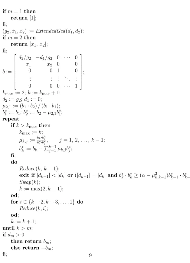
Also, because of the above discussed nature of the weighted norm, we need to compute Gram-Schmidt coefficients only for then×n submatrixb, with the last column ignored. The complete algorithm is specified in Fig. 1, with some auxiliary procedures given in Fig. 2. We use a natural pseudocode which is consistent with the GAP language ([18]), which provided our first
develop-if m= 1 then return [1]; fi; (g2, x1, x2) :=ExtendedGcd(d1, d2); if m= 2 then return [x1, x2]; fi; b:= d2/g2 −d1/g2 0 · · · 0 x1 x2 0 0 0 0 1 0 ... ... ... ... ... 0 0 0 · · · 1 ; kmax := 2; k:=kmax+ 1; d2 :=g2; d1 := 0; µ2,1 := (b1·b2)/(b1·b1); b∗ 1 :=b1;b∗2 :=b2−µ2,1b∗1; repeat ifk > kmax then kmax:=k; µk,j := bk·b∗j b∗ j·b∗j, j = 1,2, . . . , k−1; b∗ k :=bk − Pk−1 j=1µk,jb∗j; fi; do Reduce(k, k−1); exit if|dk−1|<|dk| or (|dk−1|=|dk| and b∗k·b∗k ≥(α−µ2k,k−1)b∗k−1·b∗k−1) Swap(k); k:= max(2, k−1); od; for i∈ {k−2, k−3, . . . ,1}do Reduce(k, i); od; k :=k+ 1; until k > m; if dm >0 then return bm; else return−bm; fi;
Figure 1: The LLL based gcd algorithm 9
ment environment. Analogous algorithms have also been implemented in
Magma ([2]).
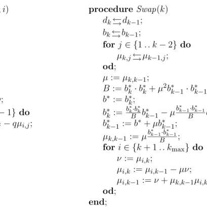
procedure Reduce(k, i) procedure Swap(k)
ifdi6= 0 then dk←→dk−1; q:=ldkdik; bk←→bk−1; else for j ∈ {1 . .k−2} do q:=dµk,ic; µk,j←→µk−1,j; fi; od; ifq 6= 0 then µ:=µk,k−1; bk :=bk −qbi; B :=b∗ k·b∗k+µ2bk∗−1·b∗k−1; µk,i :=µk,i−q; b∗ :=b∗ k; for j ∈ {1 . .i−1} do b∗ k := b∗ k·b∗k B b∗k−1−µ b∗k−1·b ∗ k−1 B b∗k; µk,j :=µk,j−qµi,j; b∗ k−1:=b∗+µb∗k−1; od; µk,k−1 :=µ b∗ k−1·b∗k−1 B ; fi; for i∈ {k+ 1 . .kmax} do end; ν :=µi,k; µi,k :=µi,k−1−µν; µi,k−1 :=ν+µk,k−1µi,k; od; end;
Figure 2: Algorithms Reduce and Swap
Experimental evidence suggests that sorting the sequence hdiimi=1 in
in-creasing order results in the fastest algorithm and tends to give better mul-tipliers than for unsorted or reverse sorted orderings.
The theoretical analysis of the LLL algorithm with α = 3/4 leads to an
O(m4log maxj{dj}) complexity bound for the time taken by this algorithm
to perform the extended gcd calculation. We can also obtain bounds on the quality of the multipliers, but these bounds seem unduly pessimistic in comparison with practical results, as is observed in other LLL applications (cf. [17]).
4
A sorting gcd approach
The presented LLL variation is very successful in obtaining small multipliers. However the quartic complexity (in terms of the number of numbers) of such an approach may be unjustified for those applications that can accept somewhat worse solutions. This is one of the reasons why we have developed a faster heuristic procedure, which we call a sorting gcd algorithm. (In fact it is quite similar to a method due to Brun [4, section 3H].)
The algorithm starts by setting up an array b, similar to the array b
created in the previous section.
b= d1 1 · · · 0 ... . .. dm 0 · · · 1
At each step the algorithm selects two rows, i and j, and subtracts rowi
from row j, some q times. Naturally, in the pessimistic case max
k {|bj,k−qbi,k|}= maxk {|bj,k|}+|q|maxk {|bi,k|}.
Once rows i and j are selected, we cannot change any individual element of either row i or j. Thus in order to minimize the damage done by a single row operation we need to minimize q. In the standard Euclidean algorithm, q is always selected as large as possible. Artificially minimizing q
by (say) selecting q to be some predefined constant may cause unacceptably long running times for the algorithm. However, by clever choice of i and
j, which minimizes q = bbj,1/bi,1c, we obtain a polynomial time algorithm,
which is quite successful in yielding “good” solutions to the extended gcd problem. Clearly, to minimize bbj,1/bi,1c, we need to select i so that bi,1
is the largest number not exceeding bj,1. This is the central idea of the
sorting gcd algorithm. In order to make the algorithm precise, we decide that the row with the largest leading element is always selected as the jth row. Throughout the algorithm, we operate on positive numbers only, i.e., we assumebi,1 ≥0, fori= 1, 2, . . . , m, and for two rowsiandj we compute
the largest q such that 0 ≤ bj,1−qbi,1 ≤ bi,1−1. Furthermore, we observe
that we can obtain additional benefits if we spread the multiplier q over several rows. This may be done whenever there is more than one row with
the same leading entry as row i. Also in such cases, the decision as to which of the identical rows to use first should be based on some norm of these rows. The distribution of the multiplierq should be then biased towards rows with smaller norm. (A discussion of relevant norms for this and related contexts appears in [7].)
An efficient implementation of the method may use a binary heap, with each row represented by a key comprising the leading element and the norm of that row with the leading element deleted, i.e.,hbi,1,||[bi,2, bi,3, . . . , bi,n+1]||i,
plus an index to it. Retrieving rowsiandj takes then at mostO(logm) time, as does reinserting them back to the heap (which occurs only if the leading element is not zero). Rowj cannot be operated upon more than logdj times and hence the complexity of the retrieval and insertion operations for all
m rows is O(mlogmlog maxj{dj}). On top of that we have the cost of
subtracting two rows, repeated at most logdj times, for each of m rows. Thus the overall complexity of the algorithm is O(m2log maxj{dj}). Subtle
changes, like spreading the multiplier q across several rows with identical leading entry, do not incur any additional time penalties in the asymptotic sense.
The following lemma gives us a rough estimate of the values that q may take. Most of the timeq =O(1), if m≥3.
LEMMA 4.1 Assume we are given a positive integer d1. The average value
of q=bd1/maxi≥2{di}c, wherehd2, . . . , dmiis a sequence ofm−1randomly
generated positive integers less than d1, is
q= Ψ(d1+ 2) +γ−1 for m= 2 ζ(m−1) +O µ m−1 (m−2)dm1−2 ¶ for m≥3 where Ψ(x)∼ln(x)− 21x −O(x−2) and ζ(k) = P∞ i=1i−k.
Outline of Proof. For the expression bd1/maxi{di}c to be equal to some q∈ {1, . . . , d1}, we must have at least onedifalling into the interval (d1/(q+
1), . . . , d1/q] and no di can be larger than d1/q. Hence the probability of
obtaining such a quotientqis equal to (1/q)m−1−(1/(q+1))m−1. The average
value of q is obtained by calculating Pd1
5
Some examples
We have applied the methods described here to numerous examples, all with excellent performance. Note that there are many papers over the years which study explicit input sets and quite a number of these are listed in the ref-erences of [4] and [15]. We illustrate algorithm performance with a small selection of examples.
Note also that there are many parameters which can affect the perfor-mance of LLL lattice basis reduction algorithms (also observed by many others, including [17]). First and foremost is the value of α. Smaller values of α tend to give faster execution times but worse multipliers, however this is by no means uniform. Also, the order of input may have an effect, as mentioned before.
(a) Take d1, d2, d3, d4 to be 116085838, 181081878, 314252913, 10346840.
Following the first method described in some detail, we see that the Kannan–Bachem algorithm gives a unimodular matrix P satisfying P A = [1,0,0,0]t: P = 2251284449726056 −1443226924799280 1 0 4502568913779963 −2886453858783690 2 0 74123990920420 −47518535244600 0 1 −90540939 58042919 0 0 .
Applying LLL with α= 3/4 to the last three rows of P gives
2251284449726056 −1443226924799280 1 0 103 −146 58 −362 −603 13 220 −144 −15 1208 −678 −381 .
Continuing the reduction with no row interchanges, shortens row 1:
−88 352 −167 −101 103 −146 58 −362 −603 13 220 −144 −15 1208 −678 −381 .
The multiplier vector −88,352,−167,−101 is the unique multiplier vector of least length, as is shown by the Fincke-Pohst method. In fact LLL-based methods give this optimal multiplier vector for all α∈[1/4,1].
Earlier algorithms which aim to improve on the multipliers do not fare particularly well. Blankinship’s algorithm ([1]) gives the multiplier vector 0, 355043097104056, 1, −6213672077130712. The algorithm due to Bradley ([3]) gives 27237259, −17460943, 1, 0. This shows that Bradley’s definition of minimal is not useful.
The gcd tree algorithm of [15] meets its theoretical guarantees and gives 0,0,6177777,−187630660. (This algorithm was not designed for practical use.)
The sorting gcd algorithm using the Euclidean norm gives −5412, 3428, 881, −26032 while it gives 3381, −49813, 27569, −3469 with the max norm. Another sorting variant gives −485, −272, 279, 1728, all of which are rea-sonable results in view of the greater speed.
There are a number of interesting comparisons and conclusions to be drawn here. First, the multipliers revealed by the first row ofP are the same as those which are obtained if we use the natural recursive approach to ex-tended gcd calculation. Viewed as an exex-tended gcd algorithm, the Kannan-Bachem algorithm is a variant of the recursive gcd and the multipliers it produces are quite poor compared to the optimal multipliers. This indicates that there is substantial scope for improving on the Kannan-Bachem method not only for extended gcd calculation but also for Hermite normal form cal-culation in general. Better polynomial time algorithms for both of these computations are a consequence of these observations. Thus, the gcd-driven Hermite normal form algorithms decribed in [9] give similar multipliers to those produced by the sorting gcd algorithm on which they are based.
(b) Taked1, . . . , d10to be 763836, 1066557, 113192, 1785102, 1470060, 3077752,
114793, 3126753, 1997137, 2603018.
The LLL-based method of section 3 gives the following multiplier vectors for various values of α. We also give the length–squared for each vector.
α multiplier vector x ||x||2 1/4 7,−1,−5,−1,−1,0,−4,0,0,0 93 1/3 −1,0,6,−1,−1,1,0,2,−3,0 53 1/2 −3,0,3,0,−1,1,0,1,−4,2 41 2/3 1,−3,2,−1,5,0,1,1,−2,−1 47 3/4 1,−3,2,−1,5,0,1,1,−2,−1 47 1 −1,0,1,−3,1,3,3,−2,−2,2 42
The Fincke-Pohst algorithm reveals that the unique shortest solution is 3,−1,1,2,−1,−2,−2,−2,2,2
which has length–squared 36. The sorting gcd algorithm using the Euclidean norm gives
−2,−3,−6,2,9,0,2,0,2,−6
with length–squared 178 while with the max norm it gives −9,5,2,−7,2,3,0,−3,−1,5
which has length–squared 207.
The recursive gcd gives multipliers
1936732230,−1387029291,−1,0,0,0,0,0,0,0,0.
The Kannan-Bachem algorithm gives
44537655090,−31896527153,0,0,0,0,0,0,0,−1.
Blankinship’s algorithm gives the multiplier vector
3485238369,1,−23518892995,0,0,0,0,0,0,0 while Bradley’s algorithm gives
−135282,96885,−1,0,0,0,0,0,0,0.
(c) The following example has theoretical significance. Taked1, . . . , dm to be
the Fibonacci numbers
(i) Fn, Fn+1, . . . , F2n, n odd,n ≥5;
(ii) Fn, Fn+1, . . . , F2n−1, n even, n ≥4.
Using the identityFmLn =Fm+n+ (−1)nFm−n, it can be shown that the
following are multipliers:
(i) −Ln−3, Ln−4, . . . ,−L2, L1,−1,1,0,0, n odd;
(ii) Ln−3,−Ln−4, . . . ,−L2,(L1+ 1),−1,0,0, n even,
where L1, L2, . . . denote the Lucas numbers 1,3,4,7, . . .
In fact we have the identities: 15
1 1 −1 0 0 · · · 0 0 0 0 0 0 0 1 1 −1 0 · · · 0 0 0 0 0 0 0 0 1 1 −1 · · · 0 0 0 0 0 0 . . . ... ... 0 0 1 1 −1 0 0 0 0 0 0 1 1 −1 Ln−1 −Ln−2 · · · L4 −L3 L2 −L1 1 −1 −Ln−3 Ln−4 · · · −L2 L1 −1 1 0 0 Fn Fn+1 . . . F2n−3 F2n−2 F2n−1 F2n = 0 0 . . . 0 0 0 1 (3) if n is odd and n≥5. 1 1 −1 0 0 · · · 0 0 0 0 0 0 0 1 1 −1 0 · · · 0 0 0 0 0 0 0 0 1 1 −1 · · · 0 0 0 0 0 0 . . . ... ... 0 0 1 1 −1 0 0 0 0 1 1 −1 −Ln−1 Ln−2 · · · L4 −L3 L2 −(L1+ 1) 1 Ln−3 −Ln−4 · · · −L2 (L1+ 1) −1 0 0 Fn Fn+1 . . . F2n−4 F2n−3 F2n−2 F2n−1 = 0 0 . . . 0 0 0 1 (4) if n is even and n ≥4.
The square matrices are unimodular, as their inverses are the following matrices, respectively: F3 F2 F5 F4 · · · Fn−3 0 −Fn−2 Fn−2 Fn F4 F3 F6 F5 · · · Fn−2 0 −Fn−1 Fn−1 Fn+1 F5−F1 F4 F7 F6 · · · Fn−1 0 −Fn Fn Fn+2 F6−F2 F5−F1 F8 F7 · · · Fn 0 −Fn+1 Fn+1 Fn+3 F7−F3 F6−F2 F9−F1 F8 · · · Fn+1 0 −Fn+2 Fn+2 Fn+4 . . . ... ... ... ... ... 0 ... ... ... Fn+1−Fn−3 Fn−Fn−4 Fn+3−Fn−5 Fn+2−Fn−6 · · · F2n−5−F1 0 −F2n−4 F2n−4 F2n−2 Fn+2−Fn−2 Fn+1−Fn−3 Fn+4−Fn−4 Fn+3−Fn−5 · · · F2n−4−F2 −1 −F2n−3 F2n−3 F2n−1 Fn+3−Fn−1 Fn+2−Fn−2 Fn+5−Fn−3 Fn+4−Fn−4 · · · F2n−3−F3 −1 −F2n−2−1 F2n−2 F2n . F3 F2 F5 F4 · · · Fn−4 −Fn−2 Fn−2 Fn−2 Fn F4 F3 F6 F5 · · · Fn−3 −Fn−1 Fn−1 Fn−1 Fn+1 F5−F1 F4 F7 F6 · · · Fn−2 −Fn Fn Fn Fn+2 F6−F2 F5−F1 F8 F7 · · · Fn−1 −Fn+1 Fn+1 Fn+1 Fn+3 F7−F3 F6−F2 F9−F1 F8 · · · Fn −Fn+2 Fn+2 Fn+2 Fn+4 . . . ... ... ... ... ... ... ... ... ... Fn−Fn−4 Fn−1−Fn−5 Fn+2−Fn−6 Fn+1−Fn−7 · · · F2n−7−F1 −F2n−5 F2n−5 F2n−5 F2n−3 Fn+1−Fn−3 Fn−Fn−4 Fn+3−Fn−5 Fn+2−Fn−6 · · · F2n−6−F2 −F2n−4−F1 F2n−4 F2n−4 F2n−2 Fn+2−Fn−2 Fn+1−Fn−3 Fn+4−Fn−4 Fn+3−Fn−5 · · · F2n−5−F3 −F2n−3−F2 F2n−3−1 F2n−3 F2n−1 .
It is not difficult to prove that the multipliers given here are the unique vectors of least length (by completing the appropriate squares and using various Fibonacci and Lucas number identities, see [10]). The length–squared of the multipliers is L2n−5 + 1 in both cases. (In practice the LLL-based
These results give lower bounds for extended gcd multipliers in terms of Euclidean norms. Since, with φ = 1+2√5,
L2n−5+ 1 ∼φ2n−5 ∼φ−5√5F2n
it follows that a general lower bound for the Euclidean norm of the multiplier vector in terms of the initial numbersdimust be at leastO(qmax{di}). Also, the length of the vector
Fn, Fn+1, . . . , F2n
is of the same order of magnitude as F2n, so a general lower bound for the
length of the multipliers in terms of the Euclidean length of the input,l say, is O(√l).
6
Conclusions
We have described new algorithms for extended gcd calculation which pro-vide good multipliers. We have given examples of their performance and indicated how the algorithms may be fully analyzed. Related algorithms which compute canonical forms of matrices will be the subject of another paper.
Acknowledgments
The first two authors were supported by the Australian Research Council.
References
[1] W.A. Blankinship, A new version of the Euclidean algorithm, Amer. Math. Mon., 70:742–745, 1963.
[2] W. Bosma and J. Cannon,Handbook of Magma functions, Department of Pure Mathematics, Sydney University, 1993.
[3] G.H. Bradley, Algorithm and bound for the greatest common divisor of
n integers, Communications of the ACM, 13:433–436, 1970. 17
[4] A.J. Brentjes, Multi–dimensional continued fraction algorithms, Math-ematisch Centrum, Amsterdam 1981.
[5] H. Cohen,A course in computational algebraic number theory, Springer– Verlag, 1993.
[6] M. Gr¨otschel, L. Lov´asz and A. Schrijver, Geometric Algorithms and Combinatorial Optimization, Springer–Verlag, Berlin 1988.
[7] G. Havas, D.F. Holt and S. Rees,Recognizing badly presentedZ-modules, Linear Algebra and its Applications, 192:137–163, 1993.
[8] G. Havas and B.S. Majewski,Integer matrix diagonalization, Technical Report TR0277, The University of Queensland, Brisbane, 1993.
[9] G. Havas and B.S. Majewski, Hermite normal form computation for integer matrices, Congressus Numerantium, 1994.
[10] V.E. Hoggatt Jr.,Fibonacci and Lucas Numbers, Houghton Mifflin Com-pany, Boston 1969.
[11] C.S. Iliopoulos. Worst case complexity bounds on algorithms for com-puting the canonical structure of finite abelian groups and the Hermite and Smith normal forms of an integer matrix, SIAM J. Computing, 18:658–669, 1989.
[12] D.E. Knuth,The Art of Computer Programming, Vol. 2: Seminumerical Algorithms, Addison-Wesley, Reading, Mass., 2nd edition, 1973.
[13] A.K. Lenstra, H.W. Lenstra Jr., and L. Lov´asz. Factoring polynomials with rational coefficients, Math. Ann., 261:515–534, 1982.
[14] L. Lov´asz and H.E. Scarf, The generalized basis reduction algorithm, Mathematics of Operations Research (1992), 17, 751–764.
[15] B.S. Majewski and G. Havas,The complexity of greatest common divisor computations, Proceedings First Algorithmic Number Theory Sympo-sium, Lecture Notes in Computer Science 877, 184–193, 1994.
[16] M. Pohst and H. Zassenhaus, Algorithmic Algebraic Number Theory, Cambridge University Press, 1989.
[17] C.P. Schnorr and M. Euchner,Lattice basis reduction: improved practical algorithms and solving subset sum problems, Lecture Notes in Computer Science 529, 68–85, 1991.
[18] M. Sch¨onert et al., GAP – Groups, Algorithms and Programming, Lehrstuhl D f¨ur Mathematik, RWTH, Aachen, 1994.
[19] C.C. Sims, Computing with finitely presented groups, Cambridge Uni-versity Press, 1994.
[20] B. Vall´ee,A Central Problem in the Algorithmic Geometry of Numbers: Lattice Reduction, CWI Quarterly (1990) 3, 95–120.