TECHNICAL UNIVERSITY OF CLUJ-NAPOCA
ACTA TECHNICA NAPOCENSIS
Series: Applied Mathematics, Mechanics, and Engineering Vol. 63, Issue I, March, 2020
PRINCIPLES OF MOTION SIMULATION OF A 2 DOF RR PLANAR
MANIPULATOR USING JAVA SWING
Tiberiu Alexandru ANTAL
Abstract: The paper presents the main differences related to a simulation made in an imperative programming language that uses 2D graphic primitives compared to the way of implementing a simulation using the Java GUI called Swing. Some basic concepts related to Java, GUIs and Swing combined with AWT are covered for a better understanding of the Java code organization for such a purpose. A 2D RR manipulator is used for computational purposes to implement object oriented the concepts in Java and to illustrate some of the simulators applications.
Key words: 2DOF, approximation, GUI, java, RR manipulator, simulation, swing, workspace.
1. INTRODUCTION
1.1Some words on the concept of GUI
The father of the GUIs is considered to be Douglas Carl Engelbart (January 30, 1925 – July 2, 2013) who was an American engineer and inventor. As a pioneer in the field of human - computer interaction, while working at ARS (Augmentation Research Center) Lab in SRI (Stanford Research Institute) International, he created the computer mouse. Engelbart, applied for the patent named “computer mouse – U.S. Patent 3,541,541” for a device described as “X-Y position indicator for a display system”, in 1967 [1] and received it in 1970. In the mid-1970s the funding of the SRI ARC Lab started to fall and many of the employees migrated to newly founded companies. One of these was Xerox PARC a part of Xerox Corporation. At the beginning of 1973, the mouse was successfully incorporated into the graphical user interface (GUI) used on the Xerox Alto - the first computer designed from the start to work with an operating system based on a graphical user interface (GUI) [2] - the father of what today we call the desktop. At that time Xerox didn’t realize the importance of the technology that had
been developed at PARC. Xerox Alto ‘commercial version’ was started to be sold in 1981, shortly before the first IBM PC was released, but somehow too late to position the product and the company in a leading position on the market of personal computers. In 1979 Steve Jobs visited Xerox PARC where he was
shown the Smalltalk-80 programming
environment, networking, and the WYSIWYG (what you see is what you get) - mouse - driven graphical user interface provided by the Alto. He sensed the importance of the GUI oriented operating seen at Xerox and demanded that these new features be integrated into their new operating system. So, the today’s GUIs are due to Engelbart who invented them, Xerox who perfected the technology and Jobs who successfully marketed the new concept.
1.2Some words on Java and the Java GUIs
object-oriented paradigm to develop software based on objects [3], [4]. When compiled, the Java source code, is translated to an intermediate representation (not a machine language) called bytecode, which can be ran only on the Java Virtual Machine (JMV). The JVM is a platform specific interpreter that runs the bytecode by turning it into machine language. Java, as all modern languages, has a very well organized CUI (Character User Interface) as well as more libraries (called packages in Java) to create GUIs (Graphical User Interface). Roughly speaking in CUI the man-machine interaction is limited the keyboard while in GUIs the mouse can be used the substitute the keyboard. Currently Java allows operation with three categories of GUIs: AWT, Swing and JavaFX. Java 1.0 contained a class library called by Sun the Abstract Window Toolkit or AWT dedicated for basic GUI programming. Technically speaking the Abstract Window Toolkit is organized around the Toolkit abstract superclass that is the base of any graphical user interface element. GUI oriented operating systems like Windows, Solaris, Macintosh provide the own GUI toolkits which are platform specific. AWT succeeded in wrapping all these into a single GUI by delegating the creation and behavior of the elements to the native (platform specific) GUI toolkit. The resulting program could run, in theory, on any of these platforms having the same “look and feel”. The problem was that graphical user interface elements such as text boxes, list boxes and menus had subtle difference in behavior on different platforms or they simply did not exist. These problems limited the usage of the AWT in achieving the “Write Once, Run Anywhere” slogan. In 1996, a company called Netscape Corporation released a graphical library called Internet Foundation Classes (IFC) which was a breakthrough. The GUI elements were painted onto windows, this way the only functionality needed from the native GUI toolkit was to create and open a window and then paint it. This entirely new design made the GUIs look and work the same no matter which platform the program ran on. Finally, from the beginning of 1997, Sun and Netscape joined their efforts and combined IFC with other technologies to form what today are called Swing and Java2D. The GUI version to
replace Swing is called JavaFX. This is intended to run on Java SE and may be used for creating and delivering desktop applications, as well as Rich Internet applications or RIA that can run across a wide variety of devices and platforms as Web, Mobile and Desktops.
1.3 Some concepts about animation and graphical simulation
Both digital animation and graphical simulation are about moving some kind of entity on the screen. Animation is related to graphics as it is a sequence of images (drawings) while a simulation can be strictly numerical or it can have also graphical parts [5] – [7]. Conceptually, the animation aims to illustrate a principle without having the intention to accurately respect the reality, while the simulation is based on some kind of mathematical model (which can describe the reality correctly and completely or only partially).
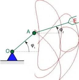
Fig. 1. – Entity types in a mechanical graphical simulation.
The graphical simulation of the mechanical systems commonly contains entities that move on the basis of some laws as well as entities that require some form of persistence. Consider the simulation from Figure 1. Here O and A are revolute joints (pivots) and point E is the end effector of this 2 DOF planar manipulator. The mathematical model for the forward kinematic problem is described by the following equations (origin is considered in O):
= cos + cos
If and lengths of the links are known, for a given set of { , } the coordinates (xE,
yE) of the E end-effector are computed directly from (1). From the simulation’s point of view (see Fig. 1) the ground link (in blue) will not move as it is fixed together with the O (green) pivot. The OA and AE (in green) links move as well as the A pivot. The E point describes a trajectory (the red curve) that must be preserved on the screen as long as the arm moves and extended based on the (1) equations each time the mechanism takes a new step (as the φ1 and φ2
angles are variated based on some law). A typical algorithm used for this would have the following pseudocode:
bg = getBackgroundColor() fg = getPenColor();
draw all still entities
for φ1 = φ1start to φ1stop step φ1step //f has some law of variation
φ2=f(φ1)
compute coord. for O, A and E if (φ1 = φ1start) then
//save the first point
Eprevious = E else
//draw a line from Eprevious //to E current to obtain //trajectory of E point
setPenColor(fg1) drawline(Eprevious,E)
//make E = E previous
Eprevious=E endif
//draw moving entities in //fg color
setPenColor(fg) drawline(OA) drawline(AE)
//wait for tms milisconds wait(tms);
//erase moving entities //by redrawing them in //bg color
setPenColor(bg) drawline(OA) drawline(AE) endfor
The graphical simulation of the RR planar manipulator movement has a numerical part based on (1) as well as a portion of drawing that is still and one that moves on the screen. Once the still entities are drawn a for loop is used to compute the positions of the moving entities (lines). The feeling of motion is obtained by drawing the entities in the foreground color (fg) waiting for a while and redrawing them in the background color (bg) to make them disappear. This general principle cannot be used under the Java GUI.
2. THE SWING GUI CONCEPT IN JAVA
Swing is a rich set of packages for creating a GUI in a platform independent way in Java. The coordinate system allows the identifications of drawn entities on the screen. By default the upper-left corner has the (0, 0) coordinates. The x coordinate is the horizontal distance moving to the right from the upper-left corner and the y coordinate is the vertical distance moving down from the upper-left corner. All graphical entities are displayed on the screen by specifying (x, y) coordinates with respect of the upper-left corner. Coordinates are measured in pixels (the monitor’s smallest unit of resolution). Pixels are positive numbers, any negative pixel values will lead the entities that will not be shown on the GUI (although these are not visible they are stored and the GUI will not give errors). Interaction with the graphical screen is handled in Java by the graphics context. The term “context” is a generic name used by the Java developers for classes that carry state information. For 2D graphics the graphics context is managed by the java.awt.Graphics
contain other user interface components (reusable software code that has a graphical representation like labels, text field, buttons, menus etc.) and not to be drawn directly by our code. Another reason would be that the drawing can overlap other user interface components of the window that can be partially or totally covered. Normally a drawing is made inside a component called panel that is added to the frame. To draw a panel the following steps should be followed:
• define a class that extends the JPanel class and add this new class to the main window;
• override the paintComponent() method of the new class with methods that draw graphical entities (lines, rectangles, ellipses and so on).
A typical code for drawing a panel is:
class NewClass extends JPanel {
public void paintComponent(Graphics g)
{
super.paintComponent(g); //methods to draw the content
//of the panel . . .
} }
The Graphics class contains the methods to manage and draw the panel with primitive graphical entities like (2D Shapes):
• g.setColor(pen) - to set the color of the pen;
• g.drawLine(x1,y1,x2,y2) - to draw a line;
• g.fillOval(x,y,w,h) - to draw a circle (if w and h are equal);
• g.drawPolyline(x[], y[], n) - to
draw a polyline stored in x[] and y[]
vectors of n elements each.
Based on the given pseudocode the simulation process in Swing seems to be simple. The appropriate drawing methods are replaced in the pseudocode and we make sure that all of them are written inside the paintComponent()
method of a class derived from a JPanel that
respects those already exposed. This would
work if all the entities in the panel were static or motionless. However, as some of the entities are moving, they should be redrawn on new positions based on (1). When motion is involved in Swing the redrawing of the panel can only be achieved by using the concept of event. Event handling is the mechanism implemented by the Swing creators to control events and to decide what should happen if an event occurs. This mechanism is based on the Delegation Event Model which defines how to generate and handle the events. Inside this model there is a separate code - known as the event handler - which is executed when an event happens. Different event sources can produce different type of events which are transmitted to event listeners that will carry out the response to the event (or handle the event). The event sources are associated to the event listeners by a process call registration. The registration is obtained by the following line of code:
eventSourceObj.addEventListener(eventSourceObj);
As Java is an object oriented language all event
objects derive from the
java.util.EventObject class. To implement an ActionListener interface the listener class
must have a method called actionPerformed()
that receives an ActionEvent object as a parameter. To successfully implement a simulation in Java using Swing and AWT we must use the javax.swing package that contains
a Timer class which can be used to update our panel contents. Java has more general-purpose timer packages however Swing timers and GUI events share the same event-dispatch thread. This means that while the Swing timer
ActionEvent is executed it can manipulate GUI
components and that the task is executed quickly. The timer has set an interval and what it should do by a class that implements the
ActionListner interface as follows:
public interface ActionListener {
void actionPerformed(ActionEvent
event); }
and notifies the ActionListener that the event
occurred. The actionPerformed() computes
based on (1) the coordinates of the A and E points and the orientation of the end-effector (positioned 7 pixels inside the AE link). The objects are then updated to the new coordinates and the AE link is stored in a Vector.
new Timer(10, new ActionListener() {
public void
actionPerformed(ActionEvent e) {
//A point
xa=x0 + rob.l * Math.cos(fi1); ya=y0 - rob.l * Math.sin(fi1);
//E point
xe=xa + rob1.l * Math.cos(fi2); ye=ya - rob1.l * Math.sin(fi2);
//E point 7 pixel back to A
xe1=xa + (rob1.l-7) * Math.cos(fi2); ye1=ya - (rob1.l-7) * Math.sin(fi2);
//Store in the objects the new // positions of A and E
rob.setXY(x0, y0, xa, ya); rob1.setXY(xa, ya, xe,ye); ef.setPosOr(-fi1, xe1, ye1);
//Store in a Vector the A, E //updated coordinates
v.addElement(new GrRobot(xa, ya,
xe,ye, getBackground(), Color.RED));
//modify the fi1 and fi2 angles fi1 += 0.002;
fi2 =
fi1*Math.sin(fi1*8.)*Math.cos(fi1/9.);
..//if fi1 exceeds the limit of 10xpi
// start from the beggining if (fi1 > 10. * Math.PI) { fi1 = 0.;
v.removeAllElements(); }
//the call of the repaint() method // it will force the call of the // paintComponent() method
repaint(); }
}).start();
The Vector class implements a one-dimensional array with variable number of object elements. Elements can be added or removed using dedicated methods of the class.
The Vector class in this application is declared as:
Vector<GrRobot> v = new Vector<GrRobot>(1);
This means that the v object is able to store one
GrRobot element from the beginning. The
addElement() method is used to add element to the Vector object. If the number of elements added is over the initial number of elements (1 in this case) the v Vector object will be re-sized automatically to fit the new required capacity. The removeAllElements() method is used to
remove all elements from the Vector object. In the previous code this method is used to reset the simulation. By clearing v the simulation loses all trajectory points being reset to the initial (void) state. The line in the actionPerformed() code is the call of the repaint method of the JPanel. This is called when we want to repaint the screen
and will cause the call of the
paintComponent() method for all component
of the object. The javax.swing.Timer has the
following constructor:
Timer(int time_in_ms, ActionListener listener);
The start() method is used start the timer
which calls the actionPerformed() method repeatedly each time the time_in_ms passes as
long as the timer is not stopped calling the
stop() method.
3. THE OBJECT ORIENTED
REPRESENTATION OF THE
MANIPULATOR
Five classes are used to achieve the graphical simulation of the manipulator: EndEffector, GroundLink, GrRobot, GrPanel which inherits from the javax.swing.JPanel class and GrFrame which inherits from the javax.swing.JFrame class. The EndEffector class stores the state of the end effector and draws the entity depending on its position an orientation as follows:
public class EndEffector { Color bck, pen;
int ypoints[]={ 5, 15, 15, 0, 15, -15, -5 };
int xpoints1[], ypoints1[]; int npoints;
public EndEffector() { npoints = xpoints.length; xpoints1 = new int[npoints]; ypoints1 = new int[npoints]; }
public void setPosOr(double fi, int tx, int ty) {
//this a pseudocode to describe the // operations on the xpoints and // ypoints arrays – the result is // stored in xpoints1 and ypoints1
Rotate(fi)
Translate(tx,ty)
}
public void draw(Graphics g) {
g.drawPolyline(xpoints1, ypoints1,
npoints); }
}
The GrRobot class stores the state and draws a pivot-link pair as follows:
public class GrRobot { int x1,y1,x2,y2; double l;
Color bck, pen;
public GrRobot(int x1, int y1, int x2, int y2, Color bck, Color pen) {
this.x1=x1; this.y1=y1; this.x2=x2; this.y2=y2; this.bck=bck; this.pen=pen; l=Math.sqrt((x1-x2)*(x1-x2)+(y1-y2)*(y1-y2));
}
public void draw(Graphics g) { //draw the link
g.setColor(pen);
g.drawLine(x1,y1,x2,y2);
//draw a white circle to cover // the line
g.setColor(Color.WHITE);
g.fillOval(x1 - 5, y1 - 5, 10, 10); //draw a black circle to show the //pivot contour
g.setColor(Color.BLACK);
g.drawOval(x1 - 5, y1 - 5, 10, 10); }
public void setXY(int x1, int y1, int x2, int y2) {
this.x1=x1; this.y1=y1; this.x2=x2; this.y2=y2; }
}
The GrPanel class contains the assembly of pivots and links assembled in the manipulator. Here, we store the states of the entities that make up the manipulator; we implement the computations used in the graphical simulation and draw on the panel the updated state of the objects forming our final scope - the motion of the manipulator. The constructor of the class is based on the following piece of code:
public GrPanel() { initComponents();
//ground link ‘center’ x0=300;
y0=250;
grlk = new GroundLink(x0,y0,70, 60 );
//pivot O and OA link
rob = new GrRobot(x0, y0, x0+50, y0…);
//pivot A and AE link
rob1 = new GrRobot(rob.x1, y0,
rob.x1+150, y0…);
//end effector (-7 pixel on AE) ef = new EndEffector();
//method call to start the timer // containing the actionEvenet() startTimer();
}
The paintComponent() method has the
following code:
public void paintComponent(Graphics g) {
super.paintComponent(g); //draw the robot
grlk.draw(g); rob.draw(g); rob1.draw(g); ef.draw(g);
if (v.size() >= 2) {
for (int i = 1; i < v.size() - 1; i++) {
p2 = v.get(i + 1); g.setColor(p1.pen);
g.drawLine(p1.x2, p1.y2, p2.x2,
p2.y2); } } }
The get() method extracts the current
position (i+1) of the end effector and the
previous one (i) in order to draw a line between
these two points. For each new position of the manipulator a new element is added to v and the for loop is redrawn from the beginning.
4. SOME APPLICATION OF THE
SIMULATOR
The applications of the simulator are related to the determination of the working space of the manipulator, of some subspaces that relate to the limitations applied to the generalized coordinates, to the obtaining of functions that approximate the working space as quickly as possible and about extending the current structures to new ones by reusing code.
4.1 Workspace determination in Swing
A typical pseudocode for determining the manipulator workspace would be:
for φ1 = φ1start to φ1stop step φ1step for φ2 = φ2start to φ2stop step φ2step solve direct kinematics(xe,ye,φ1,φ2) drawpoint(xe, ye)
endfor endfor
However such a code will not run in Swing for two reasons:
• the computational part here is timer driven (the embedded for loops that generate the set of the all possible variations of the φ1 and φ2
with a given step will run repeatedly from the beginning without advancing to the stop values);
• there is no point graphical primitive (this must be simulated using some other primitive entities from Swing).
The embedded for loops will be written as:
if (φ2 <= φ2stop)
φ2 += φ2stepp else {
φ1 += φ1step
φ2 = φ2start }
if (φ1 > φ1stop) {
φ1 = φ1start
v.removeAllElements(); }
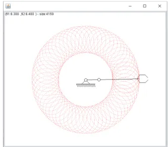
The following figures (Figure 2 to Figure 4) are showing the results of the simulations replacing the point with its equivalents available in Swing. In Figure 2 the drawLine(p1.x2, p1.y2, p1.x2, p1.y2); line of code was used in the paintComponent() method to simulate the point. This draws a line of length 1.
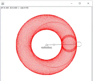
In Figure 3 the fillOval(p1.x2-2, p1.y2-2, 4,4); creates circle of radius two and, as seen, gives a better visual grasp of the simulation.
Fig. 2. – The simulation results using a line of length one instead of a point.
In Figure 4 the drawLine(p1.x2, p1.y2, p2.x2, p2.y2); draws a line between the last
Fig. 3. – The simulation results using a circle of radius two instead of a point.
Fig. 4. – The simulation results using a line that connects the previous point with the current one of the end effector.
Of the three representations of the workspace through points, raised points (circles) and lines, the lines also provide movement information (traces) compared to the first two in which only position data persists.
4.2 Subworkspace determination in Swing
Determination of subworkspaces is made by applying limitation to the pivots rotations. These limitations are defined by the start values and ending values for the rotations. In the following examples (Figure 5 to Figure 8) the initial values of the start angles are modified as follows:
double fi1 = 0.5, fi2 = 0.2;
Fig. 5. – The subworkspace simulation results using a line of length one.
Fig. 6. – The subworkspace simulation results using a circle of radius two.
while the actionPerformed() code must be updated to:
if (fi2 <= Math.PI/1.5) fi2+=0.1;
else {
fi1+=0.1;fi2=0.2; }
if (fi1 > Math.PI) return;
in order the limit the final value to Math.PI
for fi1 and to Math.PI/1.5 for fi2.
cloud can be obtained by increasing the point size.
Fig. 7. – The subworkspace simulation results using a circle of radius five.
Fig. 8. – The subworkspace simulation results using a line that connects the previous point with the current one of the end effector.
4.3 Approximate workspace computation by using a connection function between the generalized coordinates
Instead of using overlapped for loops to explore systematic and compute the workspace of the manipulator or robot with a given precision we might try to approximate the exploration procedure. The term of approximation refers to a limited number of points of the workspace computed in order to get the grasp of the entire
workspace. In Fig. 10 such a workspace is obtained by using the following code:
fi1 += 0.05;
fi2 = fi1*fi1*sin(fi1)*cos(fi1); if (fi1 > 20*Math.PI) return;
which is equivalent to the following equation:
= ∙ ∙ sin ∙ cos (2)
The two for loops from 4.1 are transformed into a single for loop as:
for φ1 = φ1start to φ1stop step φ1step
φ2 = f(φ1)
solve direct kinematics(xe,ye,φ1,φ2) drawpoint(xe, ye)
endfor
From the computational point of view this approach although it offers a partial coverage of the workspace has much shorter calculation duration. The method is important when the computation time is polynomial resulting from a large number of generalized coordinates leading to an equivalent number of entangled for cycles for obtaining the workspace.
Fig. 10. – An approximated 2D planar manipulator workspace.
preferable to the accuracy of the method, it can be applied successfully.
4.4 Reusability in simulating other manipulators (or robots)
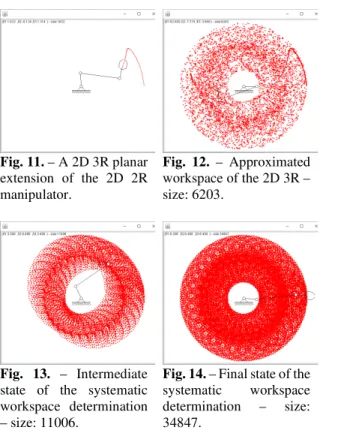
Since the implementation is object-oriented, it can be easily adapted to new structures as long as these are based on the already existing objects. Consider the simulation from Figure 11 where the 2R manipulator was extended to a 2D 3R manipulator. Figures 12 to 14 are comparing the workspace determination using the approximated and the systematic approach.
Fig. 11. – A 2D 3R planar extension of the 2D 2R manipulator.
Fig. 12. – Approximated workspace of the 2D 3R – size: 6203.
Fig. 13. – Intermediate state of the systematic workspace determination – size: 11006.
Fig. 14. – Final state of the systematic workspace determination – size: 34847.
As you can see a preliminary conclusion can be drawn from Figure 12 which used only 6203 points compared to the complete exploration from Figure 14 which used 34847 points.
5. REFERENCES
[1] https://en.wikipedia.org/wiki/ Douglas_Engelbart
[2] https://en.wikipedia.org/wiki/ PARC_(company) [3] ANTAL, T. A., Elemente de Java cu JDeveloper - îndrumător de laborator, Editura UTPRES, 2013, p.150, ISBN: 978-973-662-827-6.
[4] ANTAL, T. A., Java - Iniţiere - îndrumător de laborator, Editura UTPRES, 2013, p. 246, ISBN: 978-973-662-832-0.
[5] DETESAN, Ovidiu-Aurelian et al. THE GRAPHICAL SIMULATION OF TRR
SMALL-SIZED ROBOT. ACTA TECHNICA
NAPOCENSIS - Series: APPLIED
MATHEMATICS, MECHANICS, and
ENGINEERING, [S.l.], v. 59, n. 3, sep. 2016. ISSN 1221-5872.
[6] DETESAN, Ovidiu-Aurelian. THE
NUMERICAL SIMULATION OF TRR
SMALL-SIZED ROBOT. ACTA TECHNICA
NAPOCENSIS - Series: APPLIED
MATHEMATICS, MECHANICS, and
ENGINEERING, [S.l.], v. 58, n. 4, nov. 2015. ISSN 1221-5872.
[7] CRIŞAN, Adina - Veronica; ŞERDEAN, Florina - Maria; MORARIU - GLIGOR, Radu. THE ANALYSIS OF GEOMETRICAL ERRORS
BASED ON POLYNOMIAL
INTERPOLATION FUNCTIONS FOR A 5 D.O.F. SERIAL ROBOT. ACTA TECHNICA
NAPOCENSIS - Series: APPLIED
MATHEMATICS, MECHANICS, and
ENGINEERING, [S.l.], v. 60, n. 4, dec. 2017. ISSN 1221-5872..
Principiile simulării mişcării unui manipulator plan RR utilizând Swing Java
Lucrarea prezintă diferențele între o simulare realizată într-un limbaj de programare imperativ, care folosește primitive grafice 2D şi modul de implementare a unei simulări folosind interfaţa grafică Java numită Swing. Unele concepte de bază legate de Java, interfeţe grafice și Swing combinat cu AWT sunt prezentate pentru o mai bună înțelegere a organizării codului Java. Un manipulator plan RR este utilizat a implementa orientat pe obiect conceptele specifice simulărilor în Java și pentru a ilustra câteva dintre aplicațiile simulărilor.