Fast and efficient dense variational stereo on GPU
Julien Mairal, Renaud Keriven and Alexandre Chariot
CERTIS
ENPC
77455 Marne-la-Vallee cedex 2 France
[email protected], [email protected], [email protected]
Abstract
Thanks to their high performance and programmabil-ity, the latest graphics cards can now be used for scien-tific purpose. They are indeed very efficient parallel Sin-gle Instruction Multiple Data (SIMD) machines. This new trend is called General Purpose computation on Graphics Processing Unit (GPGPU [4]). Regarding the stereo prob-lem, variational methods based on deformable models pro-vide dense, smooth and accurate results. Nevertheless, they prove to be slower than usual disparity-based approaches. In this paper, we present a dense stereo algorithm, handling occlusions, using three cameras as inputs and entirely im-plemented on a Graphics Processing Unit (GPU). Exper-imental speedups prove that our approach is efficient and perfectly adapted to the GPU, leading to nearly video frame rate reconstruction.
1. Introduction
For the last ten years graphics cards have grown signifi-cantly in terms of performance, functionalities and relative importance in a computer.
Compared to Central Processing Units (CPUs), the growth rate has been far more higher and the GPUs do not obviously follow Moore’s law. The newest NVIDIA/ATI cards confirm this trend in terms of pipelines numbers (24/48), memory amounts (512MB), clock frequencies (650MHz), memory bandwidth (50GB/sec), etc.
The idea of using them for something else than three-dimensional rendering emerged when GPU designers made them programmable, in order to provide more expressive-ness to software developers who wanted to design their own effects.
Nevertheless, being provided with a “programmable” GPU does not mean having any generic parallel machine. A graphics card is mainly designed to render a scene and display it. Therefore, very tight constraints remain. In a
simplified view, data structures in video memory are either a set of vertices or a texture. A vertex is a set of coordinates in the three-dimensional space, augmented with attributes, such as texture coordinates or colors. A texture is an array of pixel color values, each usually composed of four chan-nels when using the RGBA mode. Moreover, because of the programming paradigm, namely the Concurrent Read Exclusive Write Single Instruction Multiple Data (CREW SIMD) programming model, only specific algorithms can be adapted and efficiently implemented on a GPU.
In this paper, we present an implementation of a dense stereo algorithm which runs entirely on a GPU. It is based on the variational framework of deformable models pro-posed by the pioneering work of [5]. In this work, the
au-thors consider then-view stereovision problem and recover
the entire surface of an object, minimizing some energy that incorporates both photometric consistency and regularizing constraints. Here, for speed reasons, we restrict ourselves to the case of two or three cameras, and model the surface as a depth map from one reference camera. Although providing smooth and accurate results for three-dimensional shape re-construction, such approaches are usually neglected in ev-eryday stereo-vision applications because of their relative lack of efficiency. This is what motivated our work. In-deed, most of the efforts that have been made toward ef-ficient stereo, are disparity-based. Instead of recovering three-dimensional information directly, the process is a two stages one: first, estimating the correspondences (dispar-ity) between two rectified images; second reconstructing the three-dimensional object. In this context, the authors of [6, 12, 7, 15, 11, 14, 13] have developed real-time or near retime stereo algorithms on GPUs. For example, the al-gorithm designed by Yang and Pollefeys in [13] can reach
up289million disparity evaluations per second on a (now
old!) ATI Radeon 9800.
Exactly like the state of the art methods classified on the reference “Middlebury Stereo Vision Page” [10], this impressive result is not focused toward accurate three-dimensional shape reconstruction. Our goal here is
differ-ent: it consists in obtaining as fast as possible a coherent and accurate surface, from two or three images or video streams. A first attempt to use GPUs for the same prob-lem has been made by the authors of [16]. Yet, although they present visibly good results, they use a non-robust dif-ference of gray levels as a photometric consistency criterion where we use instead normalized cross-correlation. Above all, the main difference between our work and theirs is that we use a mathematically founded gradient descent where they let their surface move at constant speed, just looking for a decrease of energy.
Finally, note that, although correlation based, we do nei-ther require any image rectification nor need the images be oriented the same way: the images are back-projected on the surface and correlated directly on it. To improve convergence and cope with local minima, our algorithm is multi-scale. Camera selection and occlusion are taken into account through considerations based on the normal to the surface.
2. GPU programming
2.1. Overview of GPU architecture
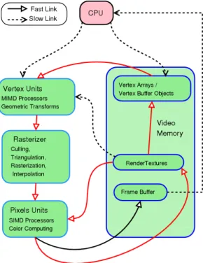
We describe here in a simplified manner the graph-ics “pipeline”. For more details, we refer the reader to [8, 1, 4, 2]. Figure 1 presents a view of a graphics card:
1. Vertices are sent to the card with directives indicating their topology (full or wireframe polygons, triangles or quads, etc.).
2. The vertex units, which are Multiple Instructions Mul-tiple Data (MIMD) processors on the latest cards, com-pute, for each vertex, a position on the screen (or on an off-screen buffer), as well as some new attributes (see [8]). This first step is now programmable. Vertex pro-grams are also called vertex shaders.
3. Some operations are then performed, such as culling (discarding vertices which are out of a previously de-fined bounding box) or stencil testing (discarding ver-tices which are on a previously defined area).
4. The so-called rasterizer converts then the vertices and their topology into sets of pixels on the screen. It links the output registers of the vertex units to the input reg-isters of the pixel units so that each pixel receives in-terpolated values from the three vertices of the triangle it belongs to.
5. The pixel units, which are Single Instruction Multi-ple Data (SIMD) processors compute the color of each pixel. This step is programmable, pixels programs be-ing also called fragment shaders, and is usually the
Figure 1. A simplified view of a recent graphics pipeline
one considered for GPGPU, although the increasing programmability of vertex shaders now turns then into good GPGPU candidates in some cases.
6. The graphics card memory is mainly organized into textures that can be seen as two-dimensional arrays. Textures are used to communicate between the CPU and the GPU or between two different successive com-putations (called rendering for obvious reasons). Pix-els programs have a full random read access to textures
and exclusive write access to one location in one1
tex-ture (the previously mentioned CREW model). Ver-tex programs can access Ver-textures too, but this access is very slow.
2.2. Iterative mesh deformation
To take advantage of the efficiency of GPUs, it is essen-tial to avoid as much as possible data transfers between the GPU and the CPU: they are very slow compared to the inter-nal GPU video memory access. In the context of an iterative process like the one we will have to deal with, there are two GPU/CPU transfer issues:
1Actually, up to four textures using so-called Multiple Rendering
1. An iteration should be able to process some input data into output data available for the next iteration with-out transmitting with-output back to the CPU. When us-ing the pixels units only, data inputs and output are
stored into so-calledRender Textures(or more recently
Frame Buffer Objects(FBO)), allowing the card to ren-der into an off-screen buffer, that can be linked after-ward to an input texture register. This is the usually adopted solution. When using also the vertex units,
data inputs must be stored intoVertex Buffer Objects
(VBO), that are actually a set of vertices data into the video memory. It is possible to transfer data from pixel textures to a VBO. This is the solution we adopted: our
surface is handled through a so-called Vertex Array,
vertices attributes being stored in a VBO.
2. One needs a way to test some stopping criterion, de-spite the fact that the pixels do not communicate, with-out transmitting data back to the CPU. This is
hope-fully possible thanks to a mechanism calledocclusion
query, which counts the number of rendered pixels. It is then easy to have every single pixel artificially not rendered is some test is true, and being instantaneously warned if this test is true for all the pixels.
3. Two cameras
3.1. Model
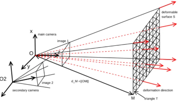
Let us consider the case where two cameras are used. Dealing with a third camera is similar and will be de-tailed further. Considering two fully-calibrated cameras and choosing camera 1 as a reference, we model the object as
a regular triangulated deformable surfaceS (see figure 2)
where each vertexM lie on a fixed ray issued from the
op-tical center O of camera 1. Although asymmetrical, this
representation spares a lot of computation. LetdM be the
distance between point O and point M. We will design
some energy E(S)that is actually a function of the dMs
and minimize it by means of a gradient descent.
3.2. Energy
The simplest energy could be the sum of the differences between the gray levels:
E(S) = Z
S
(I2◦Π2(m)−I1◦Π1(m))2dS(m)
where theIi are the images,Πi the projections associated
to the cameras and◦denotes the function composition.
Be-cause the sum is done all over the surface, one could think this measure is robust enough, like mentioned in [16]. We have tried it without success on real images. Following [5],
O z x y deformable surface S image 1 deformation direction main camera secondary camera O2 image 2 M d_M =||OM|| triangle T
Figure 2. Framework of the cameras.
we use a more robust energy, based on normalized cross-correlation, where the images are back-projected onto the
surface (or the plane tangent toSaroundm) and correlated
on some neighborhood ofm:
E(S) = Z
S
(1−ρ(I1◦Π1, I2◦Π2, m))dS(m) (1)
We choose a discrete version ofE(S), computing the
cor-relations on each triangle only. Denoting byTthe triangles
ofS, we thus take: E(S) =X T ET = X T (1−ρT(I1◦Π1, I2◦Π2)) (2)
with (omitting dependencies inTin the notations):
ρT = < I1, I2> |I1|.|I2| (3) < I1, I2> = 1 AT Z T (I1◦Π1(m)−I1◦Π1) (I2◦Π2(m)−I2◦Π2)dm Ii◦Πi = 1 AT Z T Ii◦Πi(m)dm |Ii| = p < Ii, Ii >
AT denoting the surface of triangleT. Note that we do not
use any surface metric anymore. Multiplying the correla-tion by the area of the triangle would lead to the smallest
possible surface (i.e. converging toward pointO). This
be-havior is common to all active contour based methods and is usually solved with some balloon force. We could have done this here but we got better results with above formula-tion added with some regularizaformula-tion term (see further).
3.3. Gradient
We minimize the energy by means of a gradient descent, using a multi-resolution scheme, in terms of both mesh and
image sizes, in order to cope with local minima as much as
possible. E(S)being actually a function of the distances
dMs, we have to compute its gradient with respect to these
distances. LetV(M)be the set of triangles to which a
ver-texM belongs, we write:
∂E(S) ∂dM = X T∈V(M) ∂ET ∂dM (4)
Computing these quantities from equations (2) and (3) when
M is one of the vertices ofT is straightforward but gives
rather long expressions we will not detail here. We refer the reader to [9] for their complete writing. To discuss their GPU implementation, the important fact is that they boil down to double sums (the mean values being encapsulated inside the main sum) depending on the following quantities:
∂Ii◦Πi(m)
∂dM (5)
where pointmis a point ofT andM one of its vertices.
3.4. GPU discretization
Implementing the above quantities on a GPU, the
continuous sums RTF(m)dm involved in equation (2)
for some F will indeed be replaced by discrete sums
P
pF(p)dm(p) where p is determined by the rasterizer
and each pixel shader will compute f(p). Let T be the
triangle (M1, M2, M3), p will be some barycenter p =
α1M1+α2M2+α3M3withαi≥0andα1+α2+α3= 1.
We then need to compute the quantities of equation (5), i.e. Di,k(α1, α2, α3) =
∂Ii◦Πi(p)
∂dMk
for k = 1,2,3 and every (α1, α2, α3) chosen by the
ras-terizer. A direct computation involving camera projections gives:
Di,k(α1, α2, α3) =gi(αkfi(Mk),Πi(p),(∇Ii)◦Πi(p))
wherefiandgiare simple geometric function given in [9].
Note that, when a pixel shader is called for a point p, the
valueαkis not known. Yet, it is possible to get the required
αkfi(Mk): adding a virtual attribute to the vertices and
set-ting it tofi(Mk)forMkand to0forMj(j 6=k),
automat-ically provides the interpolated quantity αkfi(Mk) when
processingp. Moreover, the rasterizer can computeΠi(p)
because Πi(p) = α1Πi(M1) +α2Πi(M2) +α3Πi(M3).
An advantage of this is that the quantities depending on the
verticesMkare computed once only by the vertex units and
not for each pointp.
Note also that, when rendering a given triangle T =
(M1, M2, M3), the three valuesDi,1,Di,2andDi,3can be
computed simultaneously for eachpthanks to vectorial
ca-pacities of the GPU. Now, choosing to render the surface
from camera 1 point of view, we get that, for a givenp∈T,
the value ofI1◦Π1(p)does not depend on the positions of
the vertices ofT, i.e:
D1,k(α1, α2, α3) = 0
3.5. Summations
EachF(p)being computed for someF by pixel shaders
for eachp∈T, we still need to recoverPp∈TF(p)dm(p).
Such a reduction is a classical problem on SIMD
ma-chines and logarithmic complexity algorithms are usually designed. Here, our triangles have a small number of pix-els thanks to our multi-scale approach adapting mesh size to image dimensions. Thus a simple pass where each pixel
shader deals with one triangle and performs a loop2over it
points is much more efficient.
We also have to sum, for each vertex, quantities over its related triangles (equation (2)). Again, vertices are now as-signed to pixel shaders that perform a loop over their re-spective triangles.
3.6. Regularization
As we mentioned previously, we left any surface metric apart and should add manually a regularization term to the energy. Mean curvature motion could be used here (or in an equivalent manner adding the area of the surface to the energy). Actually, we got better results directly smoothing
dM, adding the following term to the gradient:
K ³ ( 1 |N(M)| X M0∈N(M) dM0)−dM ´
whereN(M)is the set of the neighbors ofM andKsome
constant adapted to the considered level of detail.
3.7. Stopping criterion
An obvious stopping term based on the maximum value of the gradient gives good results. In fact, a fixed number of iterations for each level of detail gives faster convergence, yet keeping similar results.
3.8. Complete scheme
As depicted figure 3, one complete iteration is finally: 1. Assign the surface vertices to the GPU vertices and
render, computing D2,k(p),(k = 1,2,3) for every
pointp.
2. Assign the surface triangles to pixel shaders and
per-form the double summation yielding ∂ET
∂dM.
3. Assign the surface vertices to pixel shaders and per-form the neighborhood summation leading to the gra-dient ∂E∂d(S)
M . Update the vertices positiondM
accord-ing to this gradient.
4. Update the VBO containing the vertices positions and optionnaly compute a stopping criterion.
3.9. Results
Our experiments were done on a standard 3GHz PC with
a (now outdated!) NVIDIA Geforce 7800 GTX 256
graph-ics card. The OpenGL library and the Cg language were
used. I2,I1and∇I2 at the different resolutions were
pre-processed in a first step. The textures were in a 16 bits mode
(yielding40%faster programs). We obtained a fast
conver-gence with an average 10 iterations per level of detail. Our multi-resolution approach proved to prevent from converg-ing toward a local minimum.
As a reference, we developed a CPU version minimiz-ing the same energy than the GPU version. This version was cautiously written and compiled with the latest compil-ers with all of the optimizations turned on. Table 1 shows the speedups between CPU and GPU versions. For each level of detail, the image and mesh resolutions are given. We observed a mean speedup of 10 times to 15 times. This shows that our implementation makes the most of the graph-ics pipeline.
Some results and total running times are given on figures 7, 8, 9 and 10.
For each presented result, we ran about 8 iterations for each level of detail mentioned table 1 except for the two
last level of detail that are run respectively4and2times.
A total running time of about250ms is observed for global
convergence. As expected, our algorithm is not as fast as those dealing with disparity maps. Again, we insist that our targeted applications are different.
A drawback so far is that we do not handle occlusions. We could easily prevent the algorithm taking occluded tri-angles into account. We will do it show in the next section when using a third camera.
4. Three cameras - Occlusions
Our model can easily be extended to three cameras. Let
us denote them C, R and L, respectively a ”center”, a
”right” and a ”left” cameras.Cwill be the reference camera
(the role played previously by camera 1) and the correlation
will be computed between cameras C andR or between
camerasCandL. Note that the cameras do not have to be
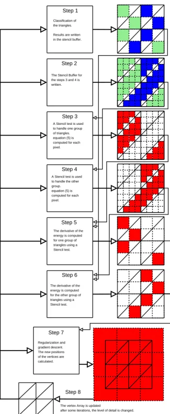
Pixel processing : (one pixel per triangle) Calculation of the new derivatives of the energy for each triangle using results of step 1 in a texture.
(note : A MRT is used.)
Pixel processing : one pixel per true surface vertex.
The regularization term is added, the gradient descent is performed. A new position for each vertex is calculated.
Step 4
The vertex Array is updated. Data from the pixel texture is copied to the VBO.
Step 4 bis (optional)
A Stop test is performed thanks to an Occlusion Query True surface
rasterization.
Pixel processing. for each pixel m of image 2, equation (5) is calculated (except for diagonals) Step 1 Step 2 Step 3 Pixel texture Pixel texture Pixel texture
Figure 3. Example of one iteration for a mesh of 3x3 vertices and an image of 8x8 pixels. Actually, our implementation begins with a 3x3 mesh and a 32x32 image. On this fig-ure, a red quad in dotted line represents one rendered pixel. The plain lines represent the mesh.
Image Mesh GPU CPU Speedup 642 52 1.60 kHz 555 Hz 2.9 1282 92 1.33 kHz 116 Hz 11.5 2562 172 464 Hz 28.6 Hz 16.2 5122 332 102 Hz 7.5 Hz 14.1 5122 652 89.4 Hz 7.3 Hz 12.2 5122 1292 67.9 Hz 7.2 Hz 9.0
Table 1. Iterations per seconds for each level of detail.
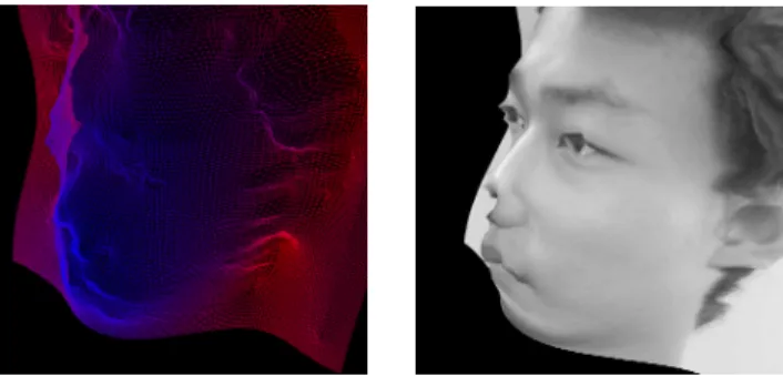
Figure 4. First and second data sets.
Figure 5. Third and fourth data sets (cour-tesy of Pr. Kyros Kutulakos (University of Toronto)).
Figure 6. A data set for three cameras from [3].
Figure 7. 240ms, two cameras.
Figure 8. 250ms, two cameras.
Figure 9. 230ms, two cameras.
disposed in a (left, center, right) way. The only criteria to assign the cameras are that: (i) the surface is modeled from
the optical center ofC, and (ii) correlation betweenLand
Ris not taken into account.
This choice being done, we divide at each iteration the
triangles into two setsSRandSL,SR(respectivelySL)
be-ing the set of the triangles that will be correlated between
cameraCand cameraR(respectively cameraL). The
as-sociated energy is indeed similar to the one given equation (2):
E(S) = PT∈SR(1−ρT(IC◦ΠC, IR◦ΠR))
+PT∈SL(1−ρT(IC◦ΠC, IL◦ΠL))
In our tests, we simply use the normal to the triangles to
choose the best secondary camera,RorL. Moreover,
oc-clusions can easily be taken into account. Rendering the surface from secondary cameras viewpoints, we determine whether a triangle is seen or not from them. When a trian-gle is not seen by any secondary camera, we just assign it
neither to SR nor toSL. Then, keeping the energy given
by equation (6), a triangle that is not seen by at leastCand
another camera does not contribute to the energy. Actually, we ignore also triangles that are not enough ”in front of” the cameras in a certain sense. This yields a first way to handle discontinuities, an important point that our model does not take into account so far.
We have implemented this algorithm on both CPU and GPU. The CPU version does not take occlusions into ac-count (a CPU visibility test would be too slow) and runs
only9%slower than its two cameras version.
Figure 11. Two cameras with occluded areas
To implement the GPU version, we use a so-called
Sten-cil Buffer to classify the triangles into two groups, being then able to work on one group only at a time. This
func-tionality consist in discarding the rendering of a pixel p
when the value of the stencil buffer at p is below, equal
to or greater than some reference value. The solution is thus to memorize in the stencil buffer whether a pixel (or
a triangle) belongs toSR, toSL or to none of them. This
Figure 12. Three cameras.
test is hardware implemented and is therefore very fast. An overview of the algorithm for the GPU version is given
fig-ure 13. Note that rendering pixels in two passes (first SR
and then SL) could lead to memory cache inefficiency if
the pixels were randomly distributed betweenSRandSL.
Hopefully, this is not the case here! Our first results show a 30% overhead between the two and three cameras GPU versions. We are still in the process of designing a more optimized three cameras GPU version.
A first result is presented figures 11 and 12. Thanks to occlusion handling, but also thanks to more precision where the three cameras are available, the three cameras recon-struction (fig. 12) is more correct and more accurate than the two cameras one (fig. 11).
5. Videos
We have tested our algorithm on video sequences.
Con-vergence on the first frame takes about250ms. Yet,
tak-ing advantage of temporal continuity, we just take the
sur-face recovered at timetas an initial value for convergence
at timet+ 1. Some preliminary tests, essentially
consist-ing in adjustconsist-ing choices of levels of detail and number of
iterations, showed promising results at a rate of 8 frames
per second for the two cameras algorithm. With the re-cently available graphics cards a 12 frames/sec rate should already be possible. Moreover, it should be noted that our approach could easily be turned into a parallel version us-ing two graphics cards with a minimum of communication at each iteration, yielding full video rate for a very afford-able price.
6. Conclusion
In this paper, we have presented a fast dense stereo algo-rithm based on variational principles. Handling occlusions, it takes two or three cameras as inputs and is entirely imple-mented on Graphics Processing Units. Experiments show that it is efficient and well adapted to the GPU: speedup of about 10 to 15 times are coherent with the graphics card we
The vertex Array is updated
after some iterations, the level of detail is changed.
Step 1 Step 2 Step 3 Step 4 Step 5 Step 6 Step 7 Step 8 Classification of the triangles. Results are written in the stencil buffer.
The Stencil Buffer for the steps 3 and 4 is written.
A Stencil test is used to handle one group of triangles. equation (5) is computed for each pixel.
A Stencil test is used to handle the other group. equation (5) is computed for each pixel.
The derivative of the energy is computed for one group of triangles using a Stencil test.
The derivative of the energy is computed for the other group of triangles using a Stencil test.
Regularization and gradient descent. The new positions of the vertices are calculated.
Figure 13. The GPU implementation with three cameras.
used. The reconstructed surface is accurate. This fully jus-tifies considering this approach instead of usual disparity-based algorithms for certain applications. Taking advan-tage of temporal continuity, we achieved reconstruction at a video rate of about 8 frames/sec. Future work includes taking discontinuities into account, dealing with more than one GPU, and investigating the reconstruction of a complete object several such systems.
References
[1] Opengl specifications. [2] http://developer.nvidia.com. [3] http://www.cs.ust.hk/∼quan/WebPami/ pami.html. [4] http://www.gpgpu.org.[5] O. D. Faugeras and R. Keriven. Variational principles, sur-face evolution, pdes, level set methods, and the stereo prob-lem. IEEE Transactions on Image Processing, 7(3):336– 344, 1998.
[6] I. Geys, T. P. Koninckx, and L. V. Gool. Fast interpolated cameras by combining a gpu based plane sweep with a
max-flow regularisation algorithm. In3DPVT ’04: Proceedings
of the 3D Data Processing, Visualization, and Transmission, 2nd International Symposium on (3DPVT’04), pages 534– 541, Washington, DC, USA, 2004. IEEE Computer Society. [7] M. Gong and Y.-H. Yang. Near real-time reliable stereo
matching using programmable graphics hardware. InCVPR
’05: Proceedings of the 2005 IEEE Computer Society Conference on Computer Vision and Pattern Recognition (CVPR’05) - Volume 1, pages 924–931, Washington, DC, USA, 2005. IEEE Computer Society.
[8] E. Kilgariff and R. Fernando. The GeForce 6 Series GPU
Architecture, volume GPU Gems 2, chapter Chap. 30. 2005. [9] J. Mairal and R. Keriven. A gpu implementation of varia-tional stereo. Technical Report O5-13, CERTIS, November 2005.
[10] D. Scharstein and R. Szeliski. A taxonomy and evaluation
of dense two-frame stereo correspondence algorithms. Int.
J. Comput. Vision, 47(1-3):7–42, 2002.
[11] J. Woetzel and R. Koch. Multi-camera real-time depth esti-mation with discontinuity handling on pc graphics hardware, August 2004.
[12] J. Woetzel and R. Koch. Real-time multi-stereo depth es-timation on gpu with approximative discontinuity handling, March 2004.
[13] R. Yang and M. Pollefeys. A versatile stereo
implementa-tion on commodity graphics hardware. Real-Time Imaging,
11(1):7–18, 2005.
[14] R. Yang, M. Pollefeys, H. Yang, and G. Welch. A unified ap-proach to real-time, multi-resolution, multi-baseline 2d view synthesis and 3d depth estimation using commodity graph-ics hardware.
[15] C. Zach, K. Karner, and H. Bischof. Hierarchical disparity estimation with programmable 3d hardware, 2004. [16] C. Zach, A. Klaus, M. Hadwiger, and K. Karner. Accurate