Federal Reserve Bank of New York
Staff Reports
Estimating Probabilities of Default
Til Schuermann
Samuel Hanson
Staff Report no. 190
July 2004
This paper presents preliminary findings and is being distributed to economists and other interested readers solely to stimulate discussion and elicit comments. The views expressed in the paper are those of the authors and are not necessarily reflective of views at the Federal Reserve Bank of New York or the Federal Reserve System. Any errors or omissions are the responsibility of the authors.
Estimating Probabilities of Default
Til Schuermann and Samuel Hanson
Federal Reserve Bank of New York Staff Reports, no. 190
July 2004
JEL classification: G21, G28, C16
Abstract
We conduct a systematic comparison of confidence intervals around estimated probabilities of default (PD), using several analytical approaches from large-sample theory and
bootstrapped small-sample confidence intervals. We do so for two different PDestimation methods—cohort and duration (intensity)—using twenty-two years of credit ratings data. We find that the bootstrapped intervals for the duration-based estimates are surprisingly tight when compared with the more commonly used (asymptotic) Wald interval. We find that even with these relatively tight confidence intervals, it is impossible to distinguish notch-level PDs for investment grade ratings—for example, a PDAA- from a PDA+. However,
once the speculative grade barrier is crossed, we are able to distinguish quite cleanly notch-level estimated default probabilities. Conditioning on the state of the business cycle helps; it is easier to distinguish adjacent PDs in recessions than in expansions.
Correspondence to Til Schuermann, Research and Market Analysis Group, Federal Reserve Bank of New York (e-mail: til.schuermann@ny.frb.org). The authors thank Joshua
Rosenberg, Marc Saidenberg, and seminar participants at the Federal Reserve Bank of New York for their insightful comments. The authors assume responsibility for any remaining errors. The views expressed in this paper are those of the authors and do not necessarily reflect the position of the Federal Reserve Bank of New York or the Federal Reserve System.
1. Introduction
Credit risk is the dominant source of risk for banks and the subject of strict regulatory oversight and policy debate (BCBS (2001a,b)).1 Credit risk is commonly defined as the loss resulting from failure of obligors to honor their payments. Arguably a cornerstone of credit risk modeling is the probability of default. Two other components are loss-given-default or loss severity and exposure at default.2 In fact these are three of the four key parameters that make up
the internal ratings based (IRB) approach that is central to the New Basel Accord (BCBS (2003)).3 In this paper we address the issue of how to estimate the probability of default (PD) with publicly available credit ratings and explore some small sample properties of this parameter estimate. We compare analytical approaches from large sample theory with confidence intervals obtained from bootstrapping. The latter are surprisingly tight.
Regulators are of course not the only constituency interested in the properties of PD estimates. PDs are inputs to the pricing of credit assets, from bonds and loans to more sophisticated instruments such as credit derivatives, and they are needed for effective risk and capital management. However, default is (hopefully) a rare event, especially for high credit quality firms which make up the bulk of the large corporate segment in any large bank. Thus estimated PDs are likely to be very noisy. Moreover, PDs may vary systematically with the business cycle and are thus unlikely to be stable over time. There may also be other important sources of heterogeneity such as country or industry that might affect rating migration dynamics generally (i.e. not just the migration to default), as documented by Altman and Kao (1992), Nickell, Perraudin and Varotto (2000) and others. For instance, Cantor and Falkenstein (2001),
1 The typical risk taxonomy includes market, credit and operational risk. See, for instance, discussions in Crouhy,
Galai and Mark (2001) or Marrison (2002).
when examining rating consistency, document that sector and macroeconomic shocks inflate PD volatilities. How then should one go about estimating PDs with a limited amount of data?
We tackle this question using publicly available data from rating agencies, in particular credit rating histories. In this way we do not attempt to build default or bankruptcy models from firm observables but take the credit rating as a sufficient statistic for describing the credit quality of an obligor. For discussions on bankruptcy and default modeling, see for instance Altman (1968), Shumway (2001), and Hillegeist, Keating, Cram and Lundstedt (2004).
Our main contribution is a systematic comparison of confidence intervals using several analytical approaches from large sample theory as well as small-sample confidence intervals obtained from the bootstrapping. We do so for two different PD estimation methods, cohort and duration (intensity). We find that the bootstrapped intervals for the duration based estimates are surprisingly tight when compared to the more commonly used Wald interval. The less efficient cohort approach generates much wider intervals, and here the bootstrap and Wald results are quite close.
The implications of these findings are significant. Even with the tighter bootstrapped confidence intervals for the duration based estimates, it is impossible to distinguish notch-level PDs for neighboring investment grade ratings, e.g. a PDAA- from a PDA+ or even a PDA. However, once the speculative grade barrier is crossed, we are able to distinguish quite cleanly notch-level estimated default probabilities. When we condition on a common factor, namely the state of the business cycle (recession vs. expansion), we find that bootstrapped PD densities overlap significantly for investment grade, even at the whole grade level (e.g. the density for PDA estimated during a recession vs. expansion). Again, for the speculative grades the two
densities are cleanly separated, suggesting that firms with these lower credit ratings are more sensitive to systematic business cycle effects. Moreover, we find that these densities are surprisingly close to normal (Gaussian).
Our approach is closest to a recent study by Christensen, Hansen and Lando (2004) who use simulation-based methods, a parametric bootstrap, to obtain confidence sets for PD estimates obtained with the duration (intensity) based approach. Their results are similar in that the confidence sets implied by their simulation technique are also tighter than those implied by asymptotics. Our resampling-based approach may arguably be better able to pick up any small sample properties of these estimators. Moreover, we consider the impact of sample length on the ability to conduct inference on PD estimates. Finally, we take into account recent results in the statistics literature which document erratic behavior of the coverage probability of the standard Wald confidence interval by also including an alternative, the Agresti-Coull confidence interval (Agresti and Coull (1998)).
The rest of the paper will proceed as follows. In Section 2 we discuss credit ratings and transition matrices and default probabilities. Section 3 discusses properties of empirical estimates of default probabilities; here we compare analytical approaches with the bootstrap. Section 4 provides some final comments.
2. Credit ratings and transitions
Credit migration or transition matrices characterize past changes in credit quality of obligors (typically firms) using ratings migration histories. We will focus our attention on the last column of this matrix which denotes the probability of default. It is customary to use a one-year horizon in credit risk management, and we will follow suit. Lando and Skodeberg (2002)
present and review several approaches to estimating these migration matrices which are compared extensively in Jafry and Schuermann (2004). Broadly there are two approaches, cohort and two variants of duration (or hazard) – parametric (imposing time homogeneity or invariance) and nonparametric (relaxing time homogeneity). Using results from Jafry and Schuermann (2004) we conduct most of our analysis using the parametric duration or migration intensity approach with some comparison to the oft-used cohort approach.
In simple terms, the cohort approach just takes the observed proportions from the beginning of the year to the end (for the case of annual migration matrices) as estimates of migration probabilities. Suppose there are Ni firms in rating category i at the beginning of the year, and Nij migrated to grade j by year-end. An estimate of the transition probability
is ij ij i N P N
= . For example, if two firms out of 100 went from grade ‘AA’ to ‘A’, then
PAA→A = 2%. Any movements within the year are not accounted for. Typically firms whose
ratings were withdrawn or migrated to Not Rated (NR) status are removed from the sample.4 The duration approach counts all rating changes over the course of the year and divides by the time spent in the starting state or rating to obtain the migration intensity which is transformed into a migration probability. For example, if a firm begins the year in A, transitions mid-year to BBB, before ending the year in BB, both transitions (A → BBB and BBB → BB) as well as the portion of time spent in each of the three states would contribute to the estimated probabilities. In the cohort approach, the mid-year transition to BBB as well as the time spent in
4 The method which has emerged as an industry standard treats transitions to NR as non-informative. The
probability of transitions to NR is distributed among all states in proportion to their values. This is achieved by gradually eliminating companies whose ratings are withdrawn. We use this method, which appears sensible and allows for easy comparisons to other studies.
BBB would have been ignored. Moreover, firms which end the period in an NR status still contribute to the estimated probabilities up until the date when they transition to NR.5
The migration matrix can also be estimated using nonparametric methods such as the Aalen-Johansen estimator which imposes fewer assumptions on the data generating process by allowing for time non-homogeneity while fully accounting for all movements within the sample period (or estimation horizon).6 Jafry and Schuermann (2004) find that relaxing the time
homogeneity assumption by using this nonparametric estimator generates annual transition matrices that are statistically indistinguishable from their parametric counterparts. For this reason we focus our modeling efforts just on the parametric intensity approach.
2.1.Estimating confidence intervals of PDs
Once we obtain estimates of the default probabilities, we can discuss several approaches for inference and hypothesis testing. Denote PDR as shorthand for the one-year probability of default for a firm with rating R. We seek to construct a (1-α)% confidence interval, e.g. α = 5%, around an estimate of PDR: (2.1) Pr min m max 1 R R R PD PD PD α < < = −
As default rates are very small for high quality borrowers, min
R
PD may be zero, and in this way
the interval may not be symmetric about mPDR.
5 There is a range of differences between the number of firm years spent in rating i and N
i from the cohort approach
range. For instance, the total number of firm years spent in ‘BBB’ during 2002 was 857 whereas NBBB = 804 under
the cohort approach. The difference is driven by time spent in ‘BBB’ by firms in mid-year transit and by firms
whose ratings were withdrawn. By contrast, the difference for the ‘A’ rating was much smaller: 695 against NA =
694.
2.2.Confidence intervals based on theory
If default is taken to be a binomial random variable, then the standard Wald confidence interval CIW is (2.2) m m
(
m)
* 1 R R R W R PD PD CI PD N κ − = ± , where * RN is the total number of firm-years spent in rating R, and κ is the 100 1
(
−α2)
th percentileof the standard normal distribution. For example, in the case of α = 5%, κ= 1.96. Naturally this
assumes that PDmR is estimated from a set of iid draws meaning, for instance, that the probability
of default does not vary systematically across time or industry, and that the likelihood of default
for firm i in year t is independent of firm j in the same year. This clearly seems unreasonable as
there are likely to be common factors such as the state of the economy which affect all firms,
albeit differentially, in a given year t. For this reason the Wald confidence interval described by
(2.2) will likely be too tight.
With this in mind, how large does *
R
N need to be to obtain a reasonable estimate of
mR
PD ? Clearly this varies with the true PDR, but a common rule of thumb is m *
R R
PD N⋅ ≥ 10.7
As an illustration suppose that PDmR = 0.1% (or 10bp). The rule of thumb would suggest that
one would need *
R
N = 10,000! This probability of default is roughly in line with a BBB-rating.
To put this into perspective, in the 22 years of rating history data we will be using, there are just over 10,000 obligor years observed for BBB-rated companies. Obviously it would be a stretch to
assume that those 10,000 obligor years are iid draws.
2.3.Confidence intervals based on resampling
An alternative approach to obtaining confidence intervals for default probability estimates is via the bootstrap method. As it is not clear how to obtain asymptotic expressions for
mR
PD obtained via the duration or hazard approach, this is our preferred method for constructing
confidence intervals for these estimates. By resampling on the rating histories, we create B
bootstrap samples8 of size Nt each, where Nt is the number of firm-histories over some time
interval which could be a year or multiple years, compute the entire migration matrix
{
( )}
1 ( ) j B j t = P
and then focus our attention just on the last vector,
{
( )}
1 ( ) j B
j
t
=
PD , where j = 1, …, B denotes the
number of bootstrap replications. Efron and Tibshirani (1993) suggest that for obtaining standard errors for bootstrapped statistics, bootstrap replications of 200 are sufficient. For
confidence intervals, they suggest bootstrap replications of 1000.9 To play it safe we set
B = 10,000.
Ideally the data underlying the bootstrap should be independently and identically
distributed (iid). Broadly one may think of at least two sources of heterogeneity: cross-sectional
and temporal. It is difficult to impose temporal independence across multiple years, but easier at shorter horizons such as one year. We will still be subject to the effects of a common (macro-economic) factor, but this problem can be mitigated by focusing the analysis on either expansion
or recession years only, an issue to which we return in Sections 3.2 and 3.5.10 We are able to
8 A bootstrap sample is created by sampling with replacement from the original sample. For an excellent exposition
of bootstrap methods, see Efron and Tibshirani (1993).
9 Andrews and Buchinsky (1997) explore the impact of non-normality on the number of bootstraps. With
multimodality and fat tails the number of bootstrap replications often must increases two or three fold relative to the Efron and Tibshirani benchmarks.
10 Similarly Christensen, Hansen and Lando (2004) perform their bootstrap simulations by dividing their sample into
multi-year “stable” and “volatile” periods. See also Lopez and Saidenberg (2000) for a related discussion on evaluating credit models.
control for some but not all of these factors. For instance, we restrict our analysis to U.S. firms, i.e. no government entities (municipal, state or sovereign), and no non-U.S. entities, but do not perform separate analysis by industry largely for reasons of sample size. By mixing industries together, the resulting bootstrap samples will likely be noisier than they would be otherwise, biasing the analysis against finding differences.
Our method contrasts with the parametric bootstrap approach put forth in Christensen, Hansen and Lando (2004) who estimate an intensity based migration matrix using all the
available data and then generate many, say B*, synthetic rating histories from that estimated
migration matrix. From these pseudo-histories they compute B* intensity based migration
matrices and thus are able to compute a simulation-based confidence interval from the default
columns of the B* migration matrices. In this way their parametric bootstrap approach may be
thought of as simulation-based whereas ours is resampling-based.
3. Properties of empirical estimates of default probabilities
We will make use of credit rating histories from Standard & Poor’s where the total sample ranges from January 1, 1981 to December 31, 2002. Our data set is very similar to the data used in Bangia et al. (2002) and Jafry and Schuermann (2004). The universe of obligors is mainly large corporate institutions around the world. In order to examine the effect of business cycles, we will restrict ourselves to U.S. obligors only; there are 6,776 unique U.S. domiciled obligors in the sample. The resulting database has a total of 50,585 firm years of data, excluding withdrawn ratings, and a total of 842 rated defaults, yielding an average annual default rate of 1.66% for the entire sample.
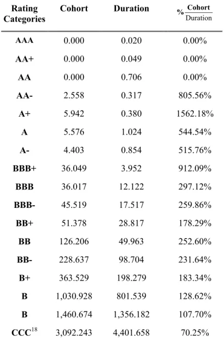
In Table 1 we present PD estimates across notch-level credit ratings using the entire sample period, 1981-2002, for both the cohort and the duration based methods with the last
column comparing the two PD estimates by grade.11 Since no defaults over one year were
witnessed for firms that started the year with a AAA, AA+ or AA ratings, the cohort estimate is
identically equal to zero, in contrast to the duration estimate where PDAAA = 0.02bp,
PDAA+ = 0.05bp and PDAA = 0.71bp. For more discussion see Jafry and Schuermann (2004).
3.1.Comparing bootstrap to analytical confidence intervals
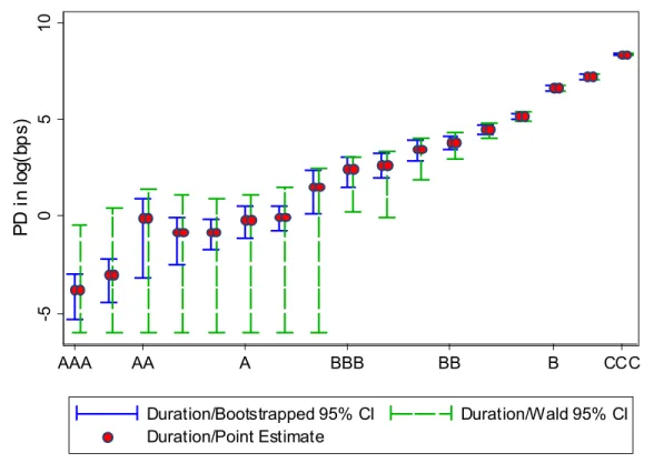
In Figure 1 we compare the bootstrap to the Wald 95% confidence interval using the
entire sample period, centered around the duration based PD point estimate presented in logs for
easier cross-grade comparison, using the number of firm-years as *
R
N in (2.2).12 We present
results at the notch level, meaning that for the AA category, for example, we show 95% bars for AA+, AA and AA-. The top and bottom grades, AAA and CCC, do not have these modifiers. The first set of bars for each pair is the interval implied by the bootstrap, the next set is the Wald interval.
Several aspects of the results are striking. First, for nearly every rating, the confidence interval implied by the bootstrap is tighter than implied by the Wald interval. For the lower
bound this may not be surprising. PDmR is small enough for the investment grades that
subtracting 1.96σˆR may indeed hit the zero boundary. For example, for grade A,
mA
PD = 0.865bp, σˆA = 1.192bp so that PDmA−1.96σˆA = -1.498bp which is clearly not possible.
11 This table is taken from Table 2 in Jafry and Schuermann (2004). All credit ratings below CCC are grouped into
Second, most of the confidence intervals, be they bootstrapped or analytical, overlap within a rating category for investment grades. In the speculative grade range one is much more clearly able to distinguish default probability ranges at the notch level. For example, the bootstrapped 95% confidence intervals for the A+, A and A- ratings almost completely overlap, implying that the estimated default probabilities for the three ratings are statistically
indistinguishable even with 22 years of data. This is not the case for B ratings, for example.
Whether one uses bootstrapped or analytical bounds, all the ratings, B+, B and B- are clearly separated.
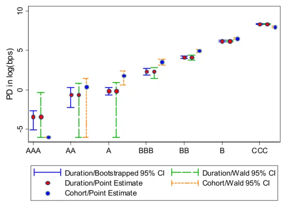
At the whole grade level, default probabilities become somewhat easier to distinguish, as can be seen from Figure 2. Here we also include cohort-based point estimates and their 95% Wald confidence intervals. No AAA defaults were observed in our sample, and hence we have no corresponding confidence interval for cohort. However, the confidence intervals for grades AA and A, whether Wald or bootstrapped, still largely overlap. Thus even at the whole grade level, dividing the investment grade into four distinct groups seems optimistic from the vantage
point of PD estimation.
At a minimum, a rating system should be ordinally consistent or monotonic meaning that
estimated PDs should be increasing as one moves from higher to lower ratings.13 Returning to
Table 1, notice that the notch-level PD estimates for both duration and cohort are not
monotonically increasing. To evaluate the issue of monotonicity more formally, we perform
12 Because the duration method makes more efficient use of rating histories than the cohort approach, *
R
N is likely
inflated, meaning that the confidence intervals will be too tight. We take up some of these issues in Section 3.6 below.
13 It is quite difficult to see how a set of estimated PDs that failed monotonicity could be consistently employed in
one-tailed tests using the bootstrap results along the following lines. For ratings k < j, where
rating k is of better credit quality (e.g. A+) than j (e.g. A), we compute the one-tailed test
(3.1) PrPDmj( )∆ <t mPDk( )∆t =α%.
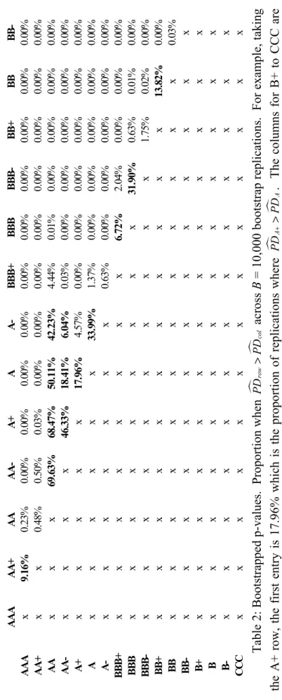
In Table 2 we report the fraction of replications for which the duration based
mj( )∆ <mk( )∆
PD t PD t over B bootstrap replications. This should be no greater than α%. We find,
in fact, that the nominal p-value often exceeds 5% for the investment grades. This is the case,
for instance, with the first test, PrPDmAA+<PDmAAA=9.16%. The nominal p-value is especially
poor for the range of AA ratings; see Section 3.4 for more discussion on behavior of this particular grade. Even the BBB grades have trouble meeting this monotonicity criterion. For
example, PrPDmBBB <PDmBBB+=6.72% and PrPDmBBB− <mPDBBB=31.90%. Only at the
non-investment grade end of the rating spectrum can we reliably state that estimated notch level PDs
are indeed monotonically increasing. Similar calculations for grade levels PDs to those shown in
Table 2 reveal that the only violation of monotonicity is between AA and A.
3.2.Common factors: recession vs. expansion
The analysis above made the arguably unrealistic assumption that all rating histories from
the whole 22 year sample period were draws from the same iid process. However, it is likely
that systematic risk factors affect all firms within a year. A simple approach may be to condition
on the state of the economy, say expansion and recession, so that defaults are conditionally
independent.14 Using the business cycle dates from the NBER,15 in the 22 years of our sample,
only 1982 was a “pure” recession year. The years 1981, 1990, 1991 and 2001 experienced a mix
of recession and expansion states. All other years are “pure” expansion years. The NBER delineates peaks and troughs of the business cycle at monthly frequencies. Since rating histories are available at a daily frequency, insofar as rating changes are dated at that level, we pick the middle of a month as the regime change from expansion to recession or vice versa.
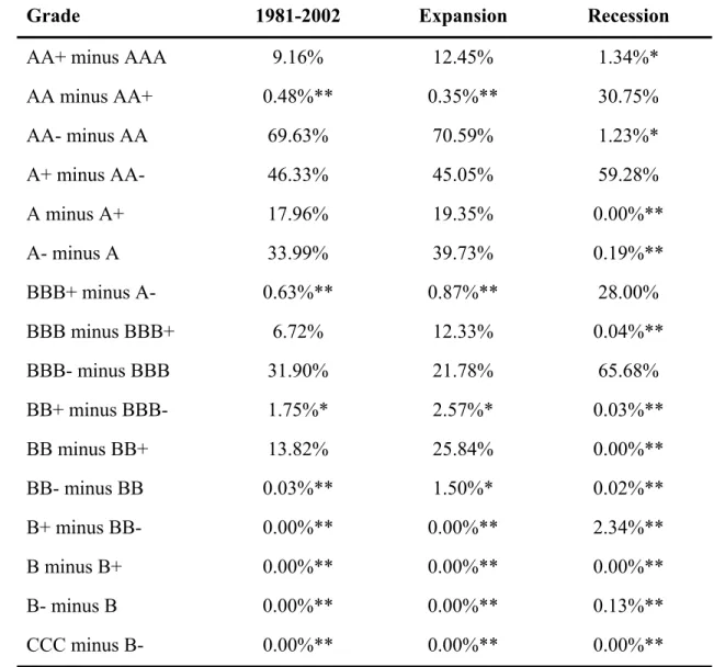
We repeat the monotonicity experiment as above, but this time we compute bootstrapped p-values separately for expansions and recessions. The results are summarized in Table 3 where we repeat in the first column labeled 1981-2002 the p-values for the whole sample range.
Conditioning on the state of the economy appears to help in differentiating PDs in adjacent credit
ratings. Of the 16 tests, half of the bootstrapped p-values exceed 5%, meaning that we would
have to reject (at the 95% level) that the two adjacent PDs are monotonic (ordinally consistent).
The proportion is the same in expansions, but conditioning on recessions reduces this proportion
to 25% (4 out of 16). For example, the unconditional PrPDmA<PDmA+=17.96%, and during
an expansion it is even worse at 19.35%, but it drops to less than 0.01% during a recession. A
similar pattern can be observed for the next pair, PrPDmA−<PDmA. Interestingly there are some
instances when monotonicity is violated in a recession but not in an expansion:
m m
PrPDBBB+ <PDA− expansion=0.87% and PrPDmBBB+<PDmA− recession=28.00%.
Speculative grade ratings are monotonic in both recessions and expansions.
3.3.Empirical densities of PDs
It may also be of interest to see how much the empirical (bootstrapped) PD distributions
for recession and expansion periods overlap. Although the rating agencies strive to achieve a
“cycle neutral” credit rating, the speculative grades tend to be more sensitive to business cycle conditions, both empirically and by design of the rating agencies (Moody’s (1999)). Thus we
would expect that the conditional PD distributions would be farther apart for speculative than for
investment grades. This is seen quite clearly in Figure 3 where we include the unconditional density for each grade for easy comparison.
For speculative grades the recession and expansion densities show very little overlap as
expected, in contrast to investment grade PDs. The multi-modality in BBB and AA ratings is a
result of default clusterings from the bootstrap; see also the discussion in Section 3.4. The unconditional and expansion densities are very close, especially for investment grade. This makes sense since we have been in an expansion most of the time (88%) since 1981. As a result the distributions for recessions are also wider than for expansions. For the A through AAA ratings, it seems that the recession densities are to the left of the expansion densities, implying
that defaults may actually be lower in recessions. Overall we find that speculative grade PDs are
more business cycle sensitive than the investment grades which is consistent with the rating agencies’ own view.
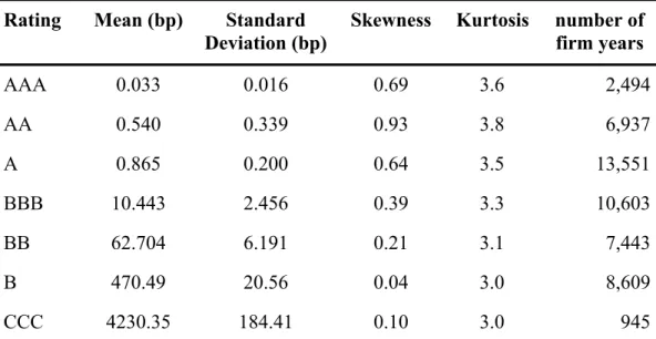
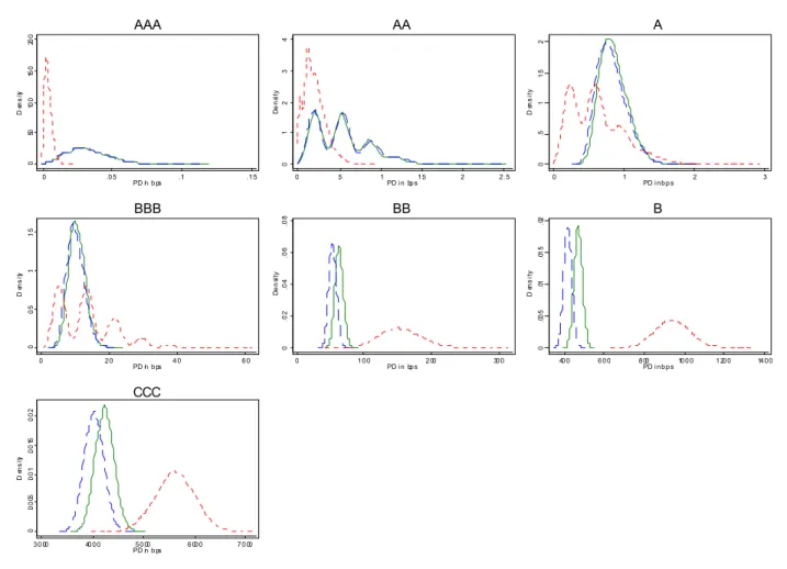
Finally, it is striking just how close to normal most of the PD densities appear to be,
especially for the speculative grades. In Figure 4 we display kernel density plots of the bootstrapped default probabilities overlaid against a normal density with the same mean and variance as a visual guide. A summary of moments for each rating is presented in Table 4. The AA grade is a glaring exception to which we will return shortly. The proximity to the normal density is perhaps especially striking for the high credit quality grades since their estimated
default probabilities are so low. The mean of our estimate of annual PDR across the 10,000
Naturally PDR can not fall below 0, so the density has a natural left (and right at 1, of course) boundary to which the investment grade densities are very close indeed. One would expect probability mass to pile up against that boundary, and we see this in the slight right skew of the investment grade densities, but this skew is indeed slight, even for AAA and A whose estimated
PDs are under a basis point.
3.4.Multi-modality of PDAA
Since we never observe a direct transition from AA+ or AA to default, our estimated PD
for AA under the duration approach primarily reflects the probability of experiencing a sequence of successive downgrades that ends in default. Thus, transitions far from the diagonal, such as
downgrades from AA to B, play a key role in determining estimated PDs for investment grade
ratings. It turns out that the multi-modal kernel density plot for AA is being driven by a single firm, TICOR Mortgage Insurance, which transitioned from AA to CCC in December of 1985. In
Figure 5 we display kernel densities for PDmAA estimated with and without TICOR. The modes
in the density plot correspond to the number of times TICOR appears in the bootstrap sample and hence the number of observed AA to CCC transitions.
We note that this not a peculiarity specific the duration method, but is due to the general difficulty of estimating probabilities for such rare events. For instance, there is a single instance of a firm beginning a year in AA- and ending the year in default (General American Life
Insurance Co. in 1999) and bootstrapped mPDAA’s from the cohort approach show a similar type
3.5.Comparing conditional and unconditional PDs
We now examine the effects of varying T, the length of the estimation window, on
grade-level PD estimates, an issue particularly relevant for practitioners. There is a trade-off between
parameter uncertainty and heterogeneity, proxied here simply by economic regime. The longer
T, the more accurate the estimates PDmR are likely to be. However, one will invariably mix
recessions (higher average PDs) and expansions (lower average PDs). If one is interested in a
long run or unconditional estimate, one would explicitly be interested in mixing these regimes. Since the average post-war recession is slightly more than one year, and the most recent two recessions have each lasted less than one year, it seems reasonable to impose conditional
independence over a one year period. Thus, comparing conditional PD estimates using rolling
one-year windows to the unconditional (i.e. full sample length) estimate seems reasonable.
In Figure 6 we compare duration (top panel) and cohort based (bottom panel) PD
estimates using a one-year rolling estimation window by grade with the unconditional estimate (reported in log basis points, bp). The CCC chart is repeated at the end in levels. Focusing first
on the top panel, for most grades we are able to reliably determine that the annual PD estimate
using just one year of data is significantly different from the long-run average for a surprisingly
large number of years. For instance, with 95% confidence we can say that the PD mB was above
its long-run average in 5 of the 22 years and below its long run average in 9 of 22 years.
Specifically, we note that the PD estimates for BB and B were significantly above their long-run
averages during 1990-1991 (there was a recession from July 1990 to March 1991), while
estimates for all grades except for AAA and AA were above their unconditional levels in 2001
the mid-1990s conditional PDs were below their unconditional levels across most ratings, consistent with the business cycle.
Looking at the top panel of Figure 6 we note that for the top two grades (and to some extent A as well) there seems to be a regime shift around 1989. Prior to that year the conditional
PD estimates were occasionally above the long run average, but since then the entire 95%
interval has been below with the single exception of AA in 2002. As discussed in section 3.4,
estimated PDs for these grade are significantly impacted by the number of transitions far from
the diagonal, particularly by downgrades of three or more grade levels, e.g. AAA → BBB.
However, such far migration have become extremely rare since 1989. This observation may be consistent with an increasing desire the part of the rating agencies to limit ratings volatility and move towards more gradual rating adjustments (Hamilton and Cantor (2004)). However, we cannot rule out the possibility that AAA and AA firms were simply subject to larger shocks during the earlier period.
The bottom panel in Figure 6 shows the one-year cohort estimates with their 95%
confidence intervals, also bootstrapped.16 The information loss incurred by applying the cohort
instead of duration based method is again striking. No defaults from AAA occurred at all in these 22 years, and only one default from AA (specifically AA- in 1999). In addition, we note
that it is more difficult to distinguish the conditional from the unconditional PD using this
estimation method.
The New Basel Accord stipulates that banks have at least five years of data on hand in order to be eligible for the advanced IRB approach (FRB (2003)). In Figure 7 we show duration
16 To be sure, the Wald intervals are quite close to and rarely smaller than the bootstrapped cohort-based confidence
based mPDs (in logs) by rating with five-year rolling estimation windows against the unconditional estimate, i.e. using the entire sample length. Again the CCC graph is repeated at the end in levels. In each case we accompany the yearly point estimates with their 95% bootstrapped confidence intervals. The unconditional estimates naturally are just a straight line across time (the x-axis). Even though we are mixing recession and expansions, nonetheless with the additional data from the wider estimation window we are still able to distinguish the
five-year conditional PD from the unconditional estimate for many of the sub-periods. The regime
shift for the highest grades mentioned above is even more pronounced in this chart, although it now appears around 1993.
3.6.Comparing (again) bootstrap to analytical confidence intervals: effect of
dependence
In Section 2.2 we introduced the Wald confidence interval for a binomial process. Brown, Cai and DasGupta (2001) show persuasively that the coverage probability of the standard Wald interval is poor not just for cases when the true (but unknown) probability is near the 0,1
boundary but throughout the unit interval.17 Among the many alternative methods for computing
a confidence interval, their final recommendation for cases where the number of observations is at least 40 is the Agresti-Coull interval, from Agresti and Coull (1998). Instead of using the
simple sample proportion, namely m R D,
R R
N PD
N
= , as the center of the confidence interval, they use
(3.2) k R D, R R N PD N = , where 2 , , / 2 R D R D N =N +κ and 2 R R N =N +κ . The corresponding confidence interval for one year is
(3.3) k kR
(
1 kR)
R AC R PD PD CI PD N κ − = ± .Agresti and Coull (1998) describe this as “add 2 successes and 2 failures” if one uses 2 instead of
1.96 for κ in the case of α = 5%. Extending (3.3) to multiple years is straight forward.
Miao and Gastwirth (2004) build on these results and explore the behavior of different interval methods in the case of dependence in the sample. They provide a dependence correction which assumes that the correlation across draws is known and confirm the recommendations in Brown, Cai and DasGupta (2001) that the (now dependence corrected) Agresti-Coull interval is preferable to the (dependence corrected) Wald interval. In both cases the correction can be most
easily formulated in terms of an adjusted number of observations †
R
N as a function of the default
correlation ρij between firm i and j:
(3.4) 2 1 † 1 2 , , R R R N N i j i R j R ij N = +
∑
< N N ⋅ρ − ,where Ni,R represents the number of trials, in our case years, for firm i with rating R. Clearly
†
R
N = NR if ρij = 0. One then uses NR† instead of NR in (2.2) and (3.2) to obtain the correlation
corrected confidence intervals. The latter becomes
k† m † 2 † 2 / 2 R R R R PD N PD N κ κ ⋅ + = + .
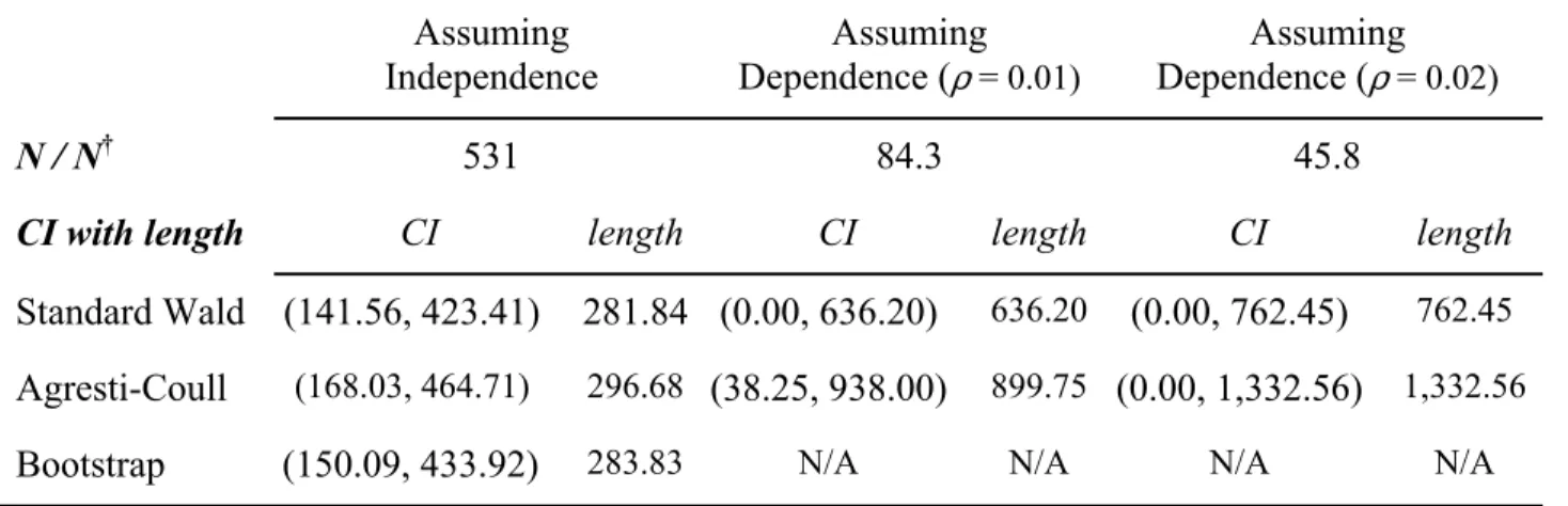
With this in mind we illustrate the impact of the different analytically based confidence intervals, with and without the assumption of dependence, for the BB-rating in the most recent year in our sample, 2002, with the bootstrap. The results are summarized in Table 5, and we use only the cohort based method since the analytical formulae are designed for the discrete binomial process rather than the continuous duration based estimate. We pick the BB-rating since we need at least some defaults to illustrate the difference between methods.
We turn our attention first to the results under the assumption of independence. The Wald and bootstrapped estimated confidence intervals are nearly of equal length, with 281.84bp and 283.83bp respectively. The analytical interval is necessarily symmetric, but not the bootstrapped interval. The Agresti-Coull interval is slightly longer at 296.68bp and is also shifted to the right, meaning that the center of the interval as well as the upper and lower bound are larger.
Even a modest default correlation of 1% can have a dramatic impact on the effective confidence interval implied by either the Wald or Agresti-Coull approach. First, the effective
number of observations †
BB
N shrinks from 531 to 84.3. The interval length more than doubles
for the standard Wald to 636.2bp and triples for the Agresti-Coull to 899.75bp. Doubling the default correlation to 2% reduces the effective number of observations to about 46, further lengthens the confidence intervals, especially the Agresti-Coull interval (namely to 1,332.56bp) so that it is bounded below at 0.
4. Concluding remarks
Using credit rating histories from S&P, we estimate probabilities of default using two estimation techniques, cohort and duration (or intensity), and compare confidence intervals for these estimates based on both analytical and bootstrap approaches. For the duration based estimates, we find that confidence intervals from bootstrapping are significantly tighter than the standard Wald intervals, which may reflect the greater efficiency of the duration approach. We next consider the effect of varying the number of grades in the rating system. We propose that rating systems should satisfy monotonicity and we test this requirement formally. Using notch
most investment grade ratings, although this criterion is generally met for speculative grade ratings. Conditioning on the state of the business cycle helps: it is easier to distinguish adjacent
PDs in recessions than in expansions.
We also consider the effects of varying the length of the estimation window to consider
conditional, i.e. time-varying, PD estimates. We compute bootstrapped confidence intervals for
intensity-based PDs estimated using one and five-year rolling windows, allowing for
comparisons between PDs estimated over these shorter intervals and their long-run averages.
For both the one and five-year windows, we are able to determine that the conditional estimate differs from the unconditional estimate for a large number of years.
Our findings have implications for regulators and credit risk practitioners alike. In a survey of internal rating systems at the fifty largest U.S. banking organizations, Treacy and Carey (2000) report that the median banking organization had five pass grades with a range from two to the low twenties. The authors also report that many banks expressed interest in increasing
the number of internal grades either through the addition of ± modifiers or by splitting riskier
grades while leaving low-risk grades intact. Our results suggest that the latter approach is to be
preferred from the vantage point of PD estimation, at least for the higher credit quality (à la
investment) grades. The addition of ± modifiers to existing low-risk ratings could result in
non-monotonic PD estimates, whereas it appears likely than meaningful estimates for additional
References
Aalen, O.O. and S. Johansen, 1978, “An Empirical Transition Matrix for Nonhomogeneous
Markov Chains Based on Censored Observations,” Scandinavian Journal of Statistics 5,
141-150.
Agresti, A. and B.A. Coull, 1998, “Approximate is Better Than ‘Exact’ for Interval Estimation of
Binomial Proportions,” The American Statistician 52, 119-126.
Altman, E.I., 1968, “Financial Ratios, Discriminant Analysis and the Prediction of Corporate
Bankruptcy,” Journal of Finance 23, 589-609.
Altman, E.I. and D.L. Kao, 1992, “Rating Drift of High Yield Bonds,” Journal of Fixed Income,
March, 15-20.
Andrews, D.W.K. and M. Buchinsky, 1997, “On the Number of Bootstrap Repetitions for Bootstrap Standard Errors, Confidence Intervals, and Tests,” Cowles Foundation Paper 1141R.
Bangia, A., F.X. Diebold, A. Kronimus and C. Schagen and T. Schuermann, 2002, “Ratings Migration and the Business Cycle, With Applications to Credit Portfolio Stress Testing,”
Journal of Banking & Finance 26 (2/3), 445-474.
Basel Committee on Banking Supervision, 2001a, The New Basel Capital Accord,
<http://www.bis.org/publ/bcbsca.htm>, January.
Basel Committee on Banking Supervision, 2001b, The Internal Ratings Based Approach,
<http://www.bis.org/publ/bcbsca.htm>, May.
Basel Committee on Banking Supervision, 2003, Third Consultative Paper,
http://www.bis.org/bcbs/bcbscp3.htm, April.
Brown, L.D., T. Cai and A. Dasgupta, 2001, “Interval Estimation for a Binomial Proportion,”
Statistical Science 16, 101-133.
Cantor, R. and E. Falkenstein, 2001, “Testing for Rating Consistency in Annual Default Rates,”
Journal of Fixed Income, September, 36-51.
Christensen, J. E. Hansen and D. Lando, 2004, “Confidence Sets for Continuous-Time Rating
Transition Probabilities,” forthcoming, Journal of Banking & Finance.
Crouhy, M., D. Galai, and R. Mark (2001), Risk Management, New York, NY: McGraw Hill.
Efron, B. and R.J. Tibshirani, 1993, An Introduction to the Bootstrap, New York, NY: Chapman
& Hall.
Federal Reserve Board, 2003, “Supervisory Guidance on Internal Ratings-Based Systems for Corporate Credit,” Attachment 2 in
http://www.federalreserve.gov/boarddocs/meetings/2003/20030711/attachment.pdf. Hamilton, D. and R. Cantor, 2004, “Rating Transitions and Defaults Conditional on Watchlist,
Hillegeist, Stephen A., Elizabeth K. Keating, Donald P. Cram and Kyle G. Lundsted, 2004,
“Assessing the Probability of Bankruptcy,” Review of Accounting Studies 9 (1), 5-34.
Jafry, Yafry and Til Schuermann, 2004, “Measurement, Estimation and Comparison of Credit
Migration Matrices,” forthcoming, Journal of Banking & Finance.
Lando, D. and T. Skodeberg, 2002, “Analyzing Ratings Transitions and Rating Drift with
Continuous Observations,” Journal of Banking & Finance, 26 (2/3), 423-444.
Lopez, J.A. and M. Saidenberg, 2000, “Evaluating Credit Risk Models”, Journal of Banking &
Finance 24 (1/2), 151-165.
Marrison, C. (2002), The Fundamentals of Risk Management, New York: McGraw Hill.
Miao, W. and J.L Gastwirth, 2004, “The Effect of Dependence on Confidence Intervals for a
Population Proportion,” The American Statistician 58, 124-130.
Moody's Investors Services (1999), Rating Methodology: The Evolving Meanings of Moody's
Bond Ratings.
Moore, D.S. and G.P. McCabe, 1993, Introduction to the Practice of Statistics, 2nd Ed., New
York: W.H. Freeman & Company.
Nickell, P, W. Perraudin and S. Varotto, 2000, “Stability of Rating Transitions,” Journal of
Banking & Finance, 24, 203-227.
Schönbucher, Philipp J., 2000, “Factor Models for Portfolio Credit Risk,” Working Paper, Department of Statistics, Bonn Univ.
Schuermann, Til, 2004, “What Do We Know About Loss Given Default?” ch. 9 in David
Shimko (ed.) Credit Risk: Models and Management, 2nd Edition, London, UK: Risk Books.
Shumway, Tyler, 2001, “Forecasting Bankruptcy more Accurately: A Simple Hazard Model,”
Journal of Business 74, 101-124.
Stein, Roger M., 2003, “Are the Probabilities Right?” Moody’s | KMV Technical Report #030124.
Treacy, W.F. and M. Carey, 2000, “Credit Risk Rating Systems at Large US Banks,” Journal of
Tables Rating Categories Cohort Duration Duration Cohort % AAA 0.000 0.020 0.00% AA+ 0.000 0.049 0.00% AA 0.000 0.706 0.00% AA- 2.558 0.317 805.56% A+ 5.942 0.380 1562.18% A 5.576 1.024 544.54% A- 4.403 0.854 515.76% BBB+ 36.049 3.952 912.09% BBB 36.017 12.122 297.12% BBB- 45.519 17.517 259.86% BB+ 51.378 28.817 178.29% BB 126.206 49.963 252.60% BB- 228.637 98.704 231.64% B+ 363.529 198.279 183.34% B 1,030.928 801.539 128.62% B 1,460.674 1,356.182 107.70% CCC18 3,092.243 4,401.658 70.25%
Table 1: Estimated Annual Probabilities of Default (PDs) in Basis Points (1981 – 2002),
across methods. S&P rated U.S. obligors. (from Table 2 in Jafry and Schuermann (2004)).
-24-Table 2: Bootstrapped p-values. Proportion when
mm row col PD PD > across B = 10,000 bootstrap replicati
ons. For exam
ple, taking
the A+ row, the first entry is 17.96% whic
h is the proportion of replications where mm AA PD PD + > . The colum ns for B+ to CCC are om itted s
ince the p-values were less than 0.0001.
A A A A A + AA AA-A+ A A -B B B + B B B B B B -B B + B B B B -AAA x 9. 16 % 0. 23 % 0. 00% 0. 00 % 0. 00% 0. 00% 0. 00 % 0. 00% 0. 00% 0. 00% 0. 00% 0. 00 % AA+ x x 0. 48 % 0. 50% 0. 03 % 0. 00% 0. 00% 0. 00 % 0. 00% 0. 00% 0. 00% 0. 00% 0. 00 % AA xxx 69 .6 3% 68 .4 7% 50 .11 % 42. 23 % 4. 44 % 0. 01% 0. 00% 0. 00% 0. 00% 0. 00 % AA -xxx x 46. 33% 18. 41 % 6. 04% 0. 03 % 0. 00% 0. 00% 0. 00% 0. 00% 0. 00 % A+ xxx xx 17. 96 % 4. 57% 0. 00 % 0. 00% 0. 00% 0. 00% 0. 00% 0. 00 % A xxx xx x 33 .9 9% 1. 37 % 0. 00% 0. 00% 0. 00% 0. 00% 0. 00 % A-x x x x x x x 0. 63 % 0. 00% 0. 00% 0. 00% 0. 00% 0. 00 % BB B+ xxx xx xxx 6. 72% 2. 04% 0. 00% 0. 00% 0. 00 % BB B xxx xx xxx x 31. 90% 0. 63% 0. 01% 0. 00 % BB B-xxx xx xxx xx 1. 75 % 0. 02 % 0. 00 % BB + xxx xx xxx xx x 13 .8 2% 0. 00 % BB xxx xx xxx xx xx 0. 03 % BB -xxx xx xxx xx xxx B+ xxx xx xxx xx xxx B xxx xx xxx xx xxx B-xxx xx xxx xx xxx CCC xxx xx xxx xx xxx
Grade 1981-2002 Expansion Recession
AA+ minus AAA 9.16% 12.45% 1.34%*
AA minus AA+ 0.48%** 0.35%** 30.75% AA- minus AA 69.63% 70.59% 1.23%* A+ minus AA- 46.33% 45.05% 59.28% A minus A+ 17.96% 19.35% 0.00%** A- minus A 33.99% 39.73% 0.19%** BBB+ minus A- 0.63%** 0.87%** 28.00% BBB minus BBB+ 6.72% 12.33% 0.04%** BBB- minus BBB 31.90% 21.78% 65.68% BB+ minus BBB- 1.75%* 2.57%* 0.03%** BB minus BB+ 13.82% 25.84% 0.00%** BB- minus BB 0.03%** 1.50%* 0.02%** B+ minus BB- 0.00%** 0.00%** 2.34%** B minus B+ 0.00%** 0.00%** 0.00%** B- minus B 0.00%** 0.00%** 0.13%** CCC minus B- 0.00%** 0.00%** 0.00%**
* and ** denote one-tailed significance of 5% and 1% respectively.
Table 3: Testing for monotonicity significance. % of bootstrap replications for rating
k < j, where k is of better credit quality (e.g. A+) than j (e.g. A) in which PDmj <PDmk. S&P credit
rating histories of U.S. firms from 1981-2002. PDs are taken from the last column of the
migration matrix estimated using the parametric intensity approach. The number of bootstrap
Rating Mean (bp) Standard Deviation (bp)
Skewness Kurtosis number of
firm years AAA 0.033 0.016 0.69 3.6 2,494 AA 0.540 0.339 0.93 3.8 6,937 A 0.865 0.200 0.64 3.5 13,551 BBB 10.443 2.456 0.39 3.3 10,603 BB 62.704 6.191 0.21 3.1 7,443 B 470.49 20.56 0.04 3.0 8,609 CCC 4230.35 184.41 0.10 3.0 945
Table 4: Empirical moments of bootstrapped probabilities of default (PDs) using S&P
credit rating histories of U.S. firms from 1981-2002. PDs are taken from the last column of the
migration matrix estimated using the parametric intensity approach. The number of bootstrap
Assuming Independence Assuming Dependence (ρ= 0.01) Assuming Dependence (ρ= 0.02) N / N† 531 84.3 45.8
CI with length CI length CI length CI length
Standard Wald (141.56, 423.41) 281.84 (0.00, 636.20) 636.20 (0.00, 762.45) 762.45
Agresti-Coull (168.03, 464.71) 296.68 (38.25, 938.00) 899.75 (0.00, 1,332.56) 1,332.56
Bootstrap (150.09, 433.92) 283.83 N/A N/A N/A N/A
Table 5: Confidence intervals for 2002 BB default probabilities in basis points estimated by cohort method.
Figures
Figure 1: Comparing asymptotic with bootstrapped 95% confidence intervals for
notch-level probabilities of default (PDs) using S&P credit rating histories of U.S. firms from
1981-2002. Note that the results are presented in log(PD) for easier comparison.
-5 0 5 10 AAA AA A BBB BB B CCC Duration/Bootstrapped 95% CI Duration/Wald 95% CI Duration/Point Estimate PD in lo g( bp s)
Figure 2: Comparing asymptotic with bootstrapped 95% confidence intervals for whole
grade-level probabilities of default (PDs) using S&P credit rating histories of U.S. firms from
1981-2002. Note that the results are presented in log(PD) for easier comparison.
-5 0 5 10 AAA AA A BBB BB B CCC Duration/Bootstrapped 95% CI Duration/Wald 95% CI
Duration/Point Estimate Cohort/Wald 95% CI
Cohort/Point Estimate P D in lo g( bp s)
Figure 3: Kernel density plots of bootstrapped probabilities of default (PDs) using S&P credit rating histories of U.S. firms from 1981-2002, split by recession and expansion. The red
line denotes recession, blue expansion, and green the unconditional density (as in Figure 4). PDs
are taken from the last column of the migration matrix estimated using the parametric intensity
approach. B = 10,000 bootstrap replication, Epanechnikov kernel using Silverman’s optimal
window. 0 50 10 0 15 0 20 0 0 .0 5 .1 .15 PD in bps D ens ity AAA 0 1 2 3 4 0 .5 1 1.5 2 2.5 PD in bps D ens it y AA 0 .5 1 1. 5 2 0 1 2 3 PD in b ps D ens it y A 0 .05 .1 .15 0 20 40 60 PD in b ps De n s ity BBB 0 .0 2 .0 4 .0 6 .0 8 0 1 0 0 2 00 300 PD in bps D ens it y BB 0 .0 0 5 .0 1 .0 1 5 .0 2 400 600 800 1000 1200 1400 PD i n bp s De n s it y B 0 .000 5 .001 .001 5 .002 3000 4000 5000 6000 70 00 PD in bps De n s ity CCC
Figure 4: Kernel density plots of bootstrapped probabilities of default (PDs) using S&P credit rating histories of U.S. firms from 1981-2002. The dashed line is the implied normal
density with the same mean and variance as the empirical density, plotted as a visual guide. PDs
are taken from the last column of the migration matrix estimated using the parametric intensity
approach. B = 10,000 bootstrap replication, Epanechnikov kernel using Silverman’s optimal
window. 0 5 10 15 20 25 De n si ty 0 .0 5 .1 .1 5 PD i n b p s AAA 0 .5 1 1. 5 2 De n s ity 0 .5 1 1 .5 2 2.5 PD in b ps AA 0 .5 1 1. 5 2 De n si ty .5 1 1 .5 2 PD i n b p s A 0 .0 5 .1 .1 5 De n si ty 0 5 10 15 2 0 2 5 PD i n b p s BBB 0 .0 2 .0 4 .0 6 .0 8 De n s ity 4 0 50 6 0 7 0 8 0 9 0 PD in b ps BB 0 .005 .0 1 .0 1 5 .0 2 De n si ty 4 00 4 50 5 0 0 55 0 PD i n b p s B 0 .0 00 5 .0 01 .0 01 5 .0 02 De n si ty 3 50 0 40 0 0 45 0 0 50 0 0 PD i n b p s CC C
Figure 5: Kernel density plots of bootstrapped AA probabilities of default (PDs) using S&P credit rating histories of U.S. firms from 1981-2002. The solid line includes the single
firm, TICOR Mortage Insurance, that migrated from AA → CCC and the modes correspond to
the number of times TICOR appears in the bootstrap sample. The dashed line repeats the same
calculation excluding TICOR. PDs are taken from the last column of the migration matrix
estimated using the parametric intensity approach. B = 10,000 bootstrap replication,
Epanechnikov kernel using Silverman’s optimal window.
0 2 4 6 0 .5 1 1.5 2 2.5 PD in bps
AA PDs incl uding TICOR AA PDs excluding TICOR
De
ns
ity
Figure 6: Comparing duration (top panel) and cohort based (bottom panel) estimates of
PD using a one-year rolling estimation windows by grade with the unconditional estimate
(reported in log basis points, bp) using S&P credit rating histories of U.S. firms from 1981-2002. The CCC chart is repeated at the end in levels.
-20 -15 -10 -5 0 1 981 1 983 1 985 19 87 19 8 9 19 9 1 1 9 9 3 1 9 95 1 9 97 1 99 9 2 00 1 PD in l og (b p s ) AAA -1 5 -1 0 -5 0 5 1 981 19 8 3 1 9 8 5 1 9 87 1 9 89 1 9 91 1 99 3 199 5 199 7 199 9 200 1 PD i n lo g (b ps ) AA -1 0 -5 0 5 19 8 1 1 9 83 1 9 85 1 98 7 198 9 19 9 1 199 3 199 5 1 997 1 9 99 2 0 01 PD in l o g( b p s ) A -10 -5 0 5 1 981 1 983 1 985 19 87 19 8 9 19 9 1 1 9 9 3 1 9 95 1 9 97 1 99 9 2 00 1 P D in lo g (bps ) BBB -2 0 2 4 6 1 981 19 8 3 1 9 8 5 1 9 87 1 9 89 1 9 91 1 99 3 199 5 199 7 199 9 200 1 P D in log( b ps ) BB 2 3 4 5 6 7 19 8 1 1 9 83 1 9 85 1 98 7 198 9 19 9 1 199 3 199 5 1 997 1 9 99 2 0 01 P D in log (bps ) B 0 2 4 6 8 10 1 981 1 983 1 985 19 87 19 8 9 19 9 1 1 9 9 3 1 9 95 1 9 97 1 99 9 2 00 1 P D in l og( bps ) CCC 0 20 00 40 00 600 0 800 0 1 981 19 8 3 1 9 8 5 1 9 87 1 9 89 1 9 91 1 99 3 199 5 199 7 199 9 200 1 PD i n (b p s ) C CC in Levels -4 -2 1 981 1 983 1 98 5 19 87 19 89 19 91 1 9 93 1 9 95 1 9 97 1 99 9 2 00 1 P D in lo g( bp s ) AAA -2 0 2 4 6 198 1 198 3 1 98 5 1 987 1 989 1 991 1 993 1 995 1 997 19 99 20 0 1 PD i n lo g (b ps ) AA 0 1 2 3 4 5 19 8 1 19 83 1 985 1 98 7 1 98 9 199 1 19 93 19 95 1 9 97 1 9 99 2 0 01 PD in l o g( b p s ) A 1 2 3 4 5 1 981 1 983 1 98 5 19 87 19 89 19 91 1 9 93 1 9 95 1 9 97 1 99 9 2 00 1 P D in lo g (bps ) BBB 0 2 4 6 8 198 1 198 3 1 98 5 1 987 1 989 1 991 1 993 1 995 1 997 19 99 20 0 1 P D in log( b ps ) BB 2 4 6 8 19 8 1 19 83 1 985 1 98 7 1 98 9 199 1 19 93 19 95 1 9 97 1 9 99 2 0 01 P D in log (bps ) B 4 5 6 7 8 9 1 981 1 983 1 98 5 19 87 19 89 19 91 1 9 93 1 9 95 1 9 97 1 99 9 2 00 1 P D in l og( bps ) CCC 0 200 0 400 0 60 00 198 1 198 3 1 98 5 1 987 1 989 1 991 1 993 1 995 1 997 19 99 20 0 1 PD i n (b p s ) CCC in Le vels
Figure 7: Comparing the 5-year rolling estimation windows by grade with the unconditional estimate (reported in log basis points, bp) using S&P credit rating histories of U.S. firms from 1981-2002. The CCC chart is repeated at the end in levels.
-15 -10 -5 0 1 981 19 83 1985 19 87 19 89 199 1 199 3 1 995 1 997 1999 2001 P D in lo g( bps ) AAA -1 0 -5 0 198 1 198 3 1985 1 987 1 989 19 91 1993 1995 199 7 199 9 2001 PD i n lo g (b ps ) AA -6 -4 -2 0 2 19 81 1983 1985 1987 1 98 9 1991 1993 1995 19 97 1999 2001 P D in lo g( bps ) A -2 0 2 4 1 981 19 83 1985 19 87 19 89 199 1 199 3 1 995 1 997 1999 2001 PD in l og (b p s ) BBB 2 3 4 5 198 1 198 3 1985 1 987 1 989 19 91 1993 1995 199 7 199 9 2001 P D i n log( bp s ) BB 5 5. 5 6 6. 5 7 19 81 1983 1985 1987 1 98 9 1991 1993 1995 19 97 1999 2001 PD in l o g( b p s ) B 6. 5 7 7. 5 8 8. 5 9 1 981 19 83 1985 19 87 19 89 199 1 199 3 1 995 1 997 1999 2001 P D in lo g( bp s ) CCC 100 0 200 0 30 00 40 00 500 0 600 0 198 1 198 3 1985 1 987 1 989 19 91 1993 1995 199 7 199 9 2001 PD i n (b p s ) C CC in Levels