Performance analysis of an optically pumped magnetometer in Earth’s magnetic field

(1)

R E S E A R C H

Open Access

Performance analysis of an optically pumped

magnetometer in Earth’s magnetic ﬁeld

Gregor Oelsner

1*

_{, Volkmar Schultze}

1

_{, Rob IJsselsteijn}

2

_{and Ronny Stolz}

1

*_{Correspondence:}

[email protected]

1_{Leibniz Institute of Photonic} Technology, Jena, Germany Full list of author information is available at the end of the article

Abstract

We experimentally investigate the influence of the orientation of optically pumped magnetometers in Earth’s magnetic field. We focus our analysis to an operational mode that promises femtotesla field resolutions at such field strengths. For this so-called light-shift dispersedMz(LSD-Mz) regime, we focus on the key parameters

defining its performance. That are the reconstructed Larmor frequency, the transfer function between output signal and magnetic field amplitude as well as the shot noise limited field resolution. We demonstrate that due to the use of two well balanced laser beams for optical pumping with different helicities the heading error as well as the field sensitivity of a detector both are only weakly influenced by the heading in a large orientation angle range.

Keywords: Optically pumped magnetometers; Heading error; Optical pumping; Bloch equations

1 Introduction

Optically pumped magnetometers (OPMs) are, in principle, scalar-type quantum sensors for magnetic fields based on the Zeeman effect. That is the shift of energy levels due to the interaction of atoms with an external magnetic field [1]. Usually alkali vapors in paraffin-coated glass cells are used as sensing element. Because the energy shift by the Zeeman interaction is based on the scalar product of the measured external magnetic fieldB0and

the magnetic moment of the atom, such a magnetometer measures the absolute value of the ﬁeld. This fact makes them interesting for the realization of absolute ﬁeld sensors [2–

4].

On the other hand, the alkali vapor is usually polarized by optical pumping with a circu-lar laser beam to create circu-large signal amplitudes. With the pump beam an additional direc-tion dependence is introduced leading besides dead zones also to unwanted effects usually summarized under the label “heading error”[5]. These effects can be understood from the change in the atom-light coupling that is in dipole approximation given by the scalar prod-uct of the laser’s electric field and the atoms electric dipole moment [6]. Suppression of the heading error is intensively studied [7–9] and it has important consequences in the application of OPMs [10,11].

(2)

The most sensitive magnetic field sensors are based on superconducting quantum inter-ference devices [12,13]. They have been optimized to allow sub-femtotesla field gradient resolution even in Earth’s magnetic field [14] and today, besides others, are used for geo-magnetic and archeological explorations [15–17]. Still the requirements due to cryogenic liquids is demanding and for low temperature superconducting sensors the costs of liquid helium are high. In this context, the newly introduced operational modes which enable shot-noise-limited field resolutions of OPMs on the femtotesla scale in Earth’s magnetic field strengths are promising alternatives. Namely, those are the light narrowing (LN) [18–

20] and the LSD-Mz [21] mode.

In this work, we analyze the performance of magnetometers based on the LSD-Mz mode and experimentally investigate their characteristics as a function of their orientation in an external magnetic field. The paper is organized as follows: We describe the experimental setup before we discuss a theoretical description of the measured values. Afterwards we present experimental data and relate it to our theoretical description. We demonstrate the influence of different rotational axis to the results. Finally, our model allows an estimate of the influence of the heading direction on the field resolution which we use to conclude on the usability of OPMs based on this mode in Earth’s magnetic field.

2 Methods

2.1 Experimental description

Because we are interested in the characteristics of a high resolution OPM as a function of its orientation relative to the Earth’s magnetic field, our experimental setup is based on a vapor cell design suitable for the LSD-Mz regime. Namely, the used micro-fabricated buffer gas cell contains two active volumes connected to the same reservoir. It is created by ultrasonic milling the desired structure into a 4 mm thick silicon wafer. The diameter of the two cylindrical cells is 11 mm and their distance 16 mm. After filling the reservoir region with droplets of diluted cesium azide and a drying step, the cell is closed by anodic bonding with Borofloat glass plates. Finally, decomposing the azide to cesium and nitrogen as buffer gas with excimer laser irradiation finalizes the fabrication. For the used cell the buffer gas pressure is about 200 mbar as necessary for the LSD-Mz mode. A detailed description of the cell fabrication can be found in [22]. A photograph of the used cell arrangement is shown in Fig.1(b).

(3)

Figure 1(a) The experimental setup (see also Ref. [6]) is mounted on a rotational table inside of a Helmholtz coil system and a mu-metal shielding. The orientation of the setup concerning the created magnetic field is adjusted by a cable pull. (b) The vapor cell used for our experimental investigations features two circularly shaped active volumes and a rectangular reservoir. (c) The schematic drawing of the setup viewed from the side for rotating angles ofα= 0 includes the optics for generating two circularly polarized laser beams. The axis of rotation is parallel to they-axis. The pump (PL) and heat laser (HL) are colored in red and blue, respectively. The whole optical setup can be rotated inside the magnetic fieldB0that is fixed along thez-axis

The pump laser (PL) with a wavelength of 895 nm is stabilized to the Doppler free ab-sorption line for theF= 3→F= 4D1transition of the Cs vapor of an additional

paraf-fin coated glass cell placed close to the laser on the optical table (not shown in Fig.1). A 978 nm heat laser is guided to the setup by a fiber and an optical setup, containing colli-mating lens and deflecting prism (not show in Fig.1). The sensor is heated to a temperature of roughly 100 degree Celsius for a suitable optical density of cesium atoms.

The whole optical installation is mounted inside of a three layer mu-metal shielding (see Fig.1(a) and Ref. [23]). Also, a three axis Helmholtz-coil system is included allowing the application of arbitrary magnetic ﬁelds. In all discussed experiments we apply a static magnetic ﬁeldB0of about 50μT along the horizontalz-axis that corresponds to the

sym-metry axis of the cylinder-shaped shields. The normal of the rotational table and thus the vertical rotational axis is labeled byy. Two additional Helmhotz coil conﬁgurations are mounted around the cell allowing for the application of magnetic rf-ﬁelds (B1)

perpendic-ular to the laser light for the detection of the magnetic resonance. We respectively denote the amplitude and the frequency of theB1ﬁeld byΩandν. Note, theB1ﬁeld created by

they-coil is perpendicular to both, laser light directionkand magnetic ﬁeldB0for each

rotation angleα. But using the second rf-coil leads to an angle modiﬁcation betweenB0

andB1from perpendicular to parallel conﬁguration during rotation. Nevertheless, we

la-bel the latter as “x-coil” according to its initial orientation. Our setup thus resembles the real situation of an OPM moved in Earth’s magnetic ﬁeld.

(4)

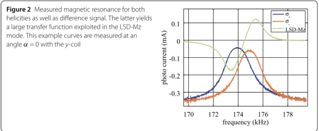
Figure 2Measured magnetic resonance for both helicities as well as diﬀerence signal. The latter yields a large transfer function exploited in the LSD-Mz mode. This example curves are measured at an angleα= 0 with they-coil

direction of the laser lightk. The latter is given bysinαex+cosαez. Here, theeidenote the

unit vectors in i-direction. Then, consecutively theB1ﬁeld is swept through the magnetic

resonance using thexas well asycoil. Thus, for each angleαrecordings are made with a magnetic rf-ﬁeld applied inyandcosαex+sinαez direction. Because at an angleα= 0

both conﬁgurations are equivalent, we adjusted the current feed to the diﬀerentB1coils

to produce magnetic resonances with the same height and width at these angles to correct for the slightly diﬀerent coil constants.

In the starting conﬁguration (α= 0) the LSD-Mz mode requires two detuned circularly polarized laser beams both of which are oriented in parallel to the external magnetic ﬁeld

B0 [21]. When using buﬀer gas cells, the population is pumped to dark states atmF =

±4 of theF= 4 ground states, respectively forσ+ andσ–light. By the magnetic rf-ﬁeld

the transition between the Zeeman-split levels can be driven, which is observable by an increase in laser absorbtion. The substraction of the signals for both helicities results in a steep linear measurement curve around the actual Larmor frequencyνL=γB0. Here

γ = 3.5 Hz/nT denotes the gyromagnetic ratio of cesium. This substraction also reduces the common noise present on the two signals, as for example intensity noise from the laser. For illustration, corresponding measurements of the magnetic resonances are presented in Fig.2for an angle ofα= 0 using they-coil.

By ﬁtting this measurement curves of the photocurrentIas a function of rf-frequency

νwith a Lorentzian function

I=I(ν) +Idc=I0

ν2

4(ν–ν0)2+ν2

+Idc, (1)

we extract the DC-photocurrentsIdc, the amplitudesI0and widths (FWHM)νof the

magnetic resonances, as well as the resonant frequenciesν0. The latter is given by the light

shifted Larmor frequencyν0=νL±νLS, whereνLSdenotes the frequency shift due to the

AC-Stark eﬀect. Although the helicity of the two laser beams as well as their relative inten-sities were balanced to less than 1% prior to recording the experimental data, a remarkable deviation in both, the dc-current and the resonance amplitude, is observed. Therefore, in all measurements including the one presented in Fig.2an additional electronic balancing through amplifying theσ+signal by an additional factor ofa= 1.61 is introduced. The

(5)

From the steepness of the diﬀerence signals=d(Iσ+–Iσ–)/dνat the Larmor frequency

we calculate the theoretical shot-noise limited sensitivity as

Bsn=

2e(Iσ+ dc(νL) +I

σ– dc(νL))

γs , (2)

by error propagation of the two channels’ shot noises where the photocurrentsIdc are

taken at the Larmor frequency andeis the elementary charge. This value sets the theoret-ical lower limit for the ﬁeld resolution of an OPM operated in the LSD-Mz mode. Please note that a possible sensor operated in theMz-mode suﬀers from low-frequency noise due

to the direct measurement of the photo-current. However, by the use of two laser beams from the same source, noise contributions such as the amplitude noise of the laser can be reduced to a large extent as we will show elsewhere. The heading characteristics of the ﬁtting parameters of Eq. (1) as well as of the sensitivity are in the following discussed.

2.2 Theoretical description

Two theoretical concepts are required for the description of our experimental results. On the one hand, the measured resonance frequencies are strongly modified by the light shift due to the intense off-resonant pumping. This effect has been extensively studied [6,7,9,

24] and we use the method presented in Ref. [6] for a description of our data.

On the other hand, the magnetic resonance itself can be described by Bloch equations. Here, we ﬁrstly analyze the Hamiltonian describing the magnetic resonance of a two-level system

H=hν0

2 σz+hΩcos2π νt[cosασx+sinασz] (3) for thex-coil. Please note that the same Hamiltonian is valid for the y-coil keepingcosα= 1 andsinα= 0. In Hamiltonian (3),Ω=γB1is introduced as the amplitude of theB1ﬁeld in

frequency units,σx,σy, as well asσzdenote Pauli matrices, andhthe Planck constant. In

order to proceed, we aim to discuss the system in a rotating frame that removes the time dependent diagonal term. That can be achieved by a unitary transformationU1=eiG(t)σz

where we chooseG(t) = Ω_ν sin2π νtcosα. As constructed,U1commutes withσz and the

termiU˙1U1†removes the diagonal coupling [25]. The transformation therefore results in

H=hν0

2 σz+hΩcos2π νtcosα

eigsin2π νtσ++e–igsin2π νtσ–

. (4)

Here, we usedσ±= 0.5(σx±iσy) and the abbreviation g=Ων cosα. Although we could

continue with the Jacobi–Anger expansion and ﬁnally ﬁnd the stationary terms in a frame rotating withν, we note that the ratioΩ/νis small in our experimental realization. Thus, we can summarize the terms in the brackets toσxand solve the Bloch equations in a frame

rotating withνaround thez-axis in rotating wave approximation. The modiﬁcation of the stationary result for thez-component of the magnetization compared to the usual result is limited to a reduction of the eﬀective rf-amplitude with a factorcosαas

σz= –

ΓrΓϕ

ΓrΓϕ+Ω2cos2α

(6)

Above we introduced the ratesΓrandΓϕas respected inverse relaxation and coherence

timesT1 andT2, as well as Γϕ= (Γϕ2+δ2)/Γϕ. The detuning of theB1 frequency from

resonance is included byδ=ν0–ν.

Still, this modiﬁcation for thex-coil alone fails to accurately explain our measured data. What is missing in Eq. (5) is the modiﬁcation of population transfer by optical pumping, or in other words the change in the dc-photocurrent that depends on the population dif-ference. To include the optical transition and the decay from the atoms excited state into the two-level model, we modify the relaxation and excitation dissipative dynamics, similar as in Refs. [26] and [27]. Namely, we set for the respective excitationΓeand decay rateΓr

Γr=

γr

2 +

Ωp|cosα|

2 (1 –cosα),

Γe=

γr

2 +

Ωp|cosα|

2 (1 +cosα).

(6)

Here we assumed a repopulation rate of the ground state levelsγr/2 and an eﬀective

pump-ing rate between the two levelsΩpproportional to the laser ﬁeldΩL(see below). We note

that the equations above are written for σ+ polarization of the light. Still, they take the

same form forσ–light. This other helicity only diﬀers by a change of the signs inside the

brackets. On the other hand, because themF = –3 level has higher energy compared to

themF= –4 in two level approximation, the result forσ–would be equivalent to Eq. (6).

The rates resulting from the optical pumping in Eq. (6) include contributions of the scalar product between the atoms’s dipole moment and the electric ﬁeld (∝1±cosα) (compare to Ref. [6]) as well as an additional factor of|cosα|. Also, we did not include the linear po-larized component scaling withsinαthat, in principle, can also contribute to a population diﬀerence. This statement is especially true close to a perpendicular pumping orientation

B0⊥ k. The rates deﬁned in (6) enter to the observable photocurrent. It relates to the

expectation value ofσzas

I(ν) =I0σz=I0

(Γe–Γr)Γϕ

(Γr+Γe)Γϕ+c2(α)Ω2

. (7)

Here, the functionc(α) is constantly one for thex-coil andcosα for they-coil. As con-structed, our model accurately describes the dc-photocurrent as shown in Sect.3. Namely, ifδ→ ±∞or equivalentlyΩ→0, we ﬁnd

Idc=I0

Γe–Γr

Γr+Γe

=I0

cos2_α

|cosα|+p1

, (8)

with the dimensionless ﬁtting parameter p1=γr/Ωp. The above function changes with

decreasing optical pumping from acosto acos2_{angular dependence while at the same}

time the amplitude is decreased. This reduction of the dc-current summarizes the fact that for an eﬀective pumping to the dark states the rate of equalization of populationγr

should be signiﬁcantly smaller than the optical pumping∝Ωp.

To bring Eq. (7) into a similar form as Eq. (1) we separate the dc-current to ﬁnd the Lorentzian-like resonance function as

I(ν) =Idc

1 – c

2₍_α₎_Ω2

(Γe+Γr)Γϕ+c2(α)Ω2

(7)

The resonance amplitude is accordingly the value of the second term in above equation at resonance, namely atν=ν0. It is

i0=I(ν=ν0)/Idc=

c2₍_α₎ c2₍_α_{) +}_p

2(p1+cosα)

, (10)

where we introduced a second dimensionless ﬁtting parameterp2=ΓϕΩp/Ω2.

Finally, the full width at half maximum (FWHM) of the resonance curve of Eq. (7) is given by

ν= 2Γϕ

1 + c

2₍_α₎ p2(p1+|cosα|)

+p3. (11)

This relation describes the quadratic addition of the natural linewidthΓϕand the power

broadening by theB1ﬁeld

νB1=

c2Γϕ

p2(p1+|cosα|))

= c

2_Ω2

Γϕ(γ+Ωp|cosα|)

(12)

of the magnetic resonance line. To ﬁt our experimental results, it is necessary to introduce an additional constant broadening termp3that we account to the broadening of the

mag-netic resonance line by the laser power as we will demonstrate below. We introduce this solely to the resonance width, since a saturation in the optical transition does not yield the same in the magnetic resonance and thus will not inﬂuence to the amplitude of the measured Lorentzian-shaped signal.

3 Results

3.1 Resonant frequency—light shift

In a first step we analyze the angular dependence of the magnetic resonance center fre-quencies as plotted in Fig.3. We added to the figure also the mean value of the measured center frequencies found for the two different circular polarizations.

In general, the magnetic resonances are strongly shifted by the ac-Stark shift due to the strong off-resonant pumping. The angle between the laser beam direction, represented by itsk-vector, and the magnetic fieldB0influences to the atom-light interaction by the

Figure 3Extracted center frequencies of the magnetic resonances for both circular polarizations of the laser as a function of the heading angleα. Also the mean frequencies of the two helicities are given. The latter roughly corresponds to the Larmor frequency measured by the LSD-Mz mode. The diamonds and dots correspond to aB1ﬁeld that is

(8)

transition dipole moment [6]

D· E= E0 2√2e

i(kr–2π νLt)_[_cos_α±_1]_D

++ [cosα∓1]D–+ 2sinαDz . (13)

ThereinE0is the amplitude of the electric ﬁeld,kthe k-vector of the laser,rthe atoms

position, νLthe frequency of the laser beam, and theDi are components of the dipole

operator. In words, above equation states that with modifying the angleαthe weight of pumping to diﬀerent excited states is strongly inﬂuenced. Namely,D+,D–, andDz

compo-nents couple to excited states with increased, decreased, as well as unchanged magnetic quantum numberm_F=mF+{+1, –1, 0}, respectively.

The strongest characteristic results from the vector light shift that can be interpreted as virtual magnetic field added in direction of the lights angular momentum [24]. It is strongest close to angles of zero and±πand reduces to zero close to perpendicular ori-entation. Also as expected, it changes its sign for a change in the laser’s helicity. A more detailed discussion of the light shift can be found in Ref. [6]. We use the findings therein to calculate the expected light-shifted transition frequencies between Zeeman levels with highest and lowest magnetic quantum numbers to their neighboring states. These corre-spond to the respective blue and orange solid lines plotted in Fig.3and can be identified with the transitions probed when pumping to the dark statesmF=±4, where the plus and

minus sign are to be used forσ+andσ–light, respectively. For the curves we used a

mag-netic ﬁeld strength ofB0= 49.664μT, detunings ofδF=4= –8 GHz andδF=3= –9.2 GHz

from the respective optical transitionsF= 4→F= 4 andF= 4→F= 3, a linewidth of the optical transitionsΓopt≈4 GHz, and optical driving amplitudes in frequency units

ΩL= 3.15 MHz and 3.45 MHz forσ+andσ–polarized beam, respectively. The last values

corresponds to the on-resonance Rabi frequencies [28] introduced by the pumping beams. We achieve a good correspondence between our model and the experimental results. It is best close to angles of zero and±π, where additionally to the strong light shift also a very good pumping to the dark states is achieved. Close to angles of±π/2, not only the ob-served light shift is reduced but also the population is distributed between several ground state levels. This eﬀect reduces the magnetic resonance amplitude and, additionally, en-ables probing more ground state transitions both reducing the agreement between theory and experiment.

Nevertheless the model allows the reconstruction of the laser intensitiesILfrom

ΩL=

1

h

IL

4cn0

J= 1/2DJ= 1/2. (14)

Here the vacuum permittivity0, speed of lightc, reduced transition dipole momentJ=

(9)

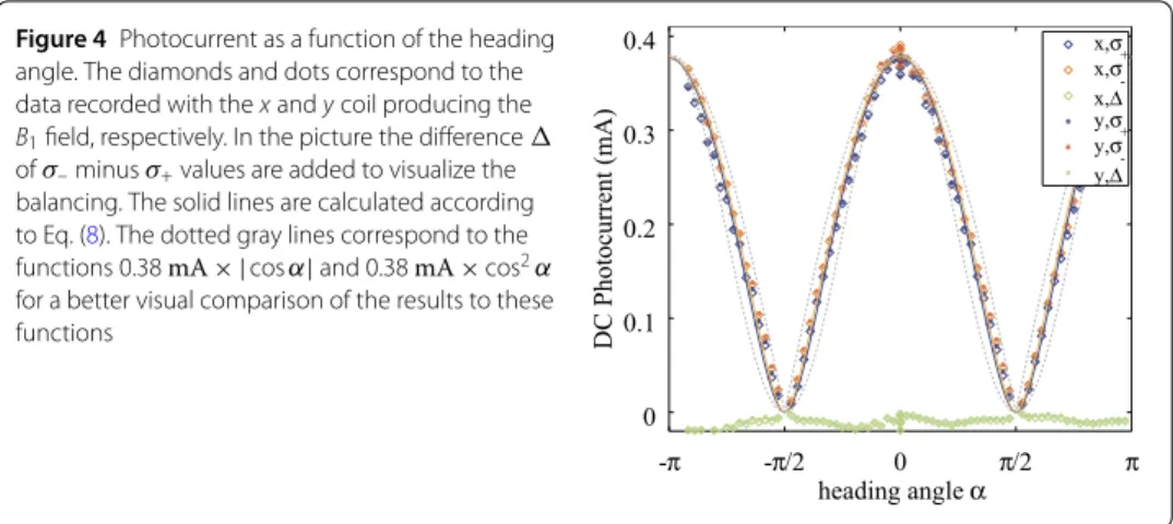
Figure 4Photocurrent as a function of the heading angle. The diamonds and dots correspond to the data recorded with thexandycoil producing the

B1ﬁeld, respectively. In the picture the diﬀerence

ofσ–minusσ+values are added to visualize the balancing. The solid lines are calculated according to Eq. (8). The dotted gray lines correspond to the functions 0.38mA× |cosα|and 0.38mA×cos2α

for a better visual comparison of the results to these functions

3.2 The dc-photocurrent

A second basic characteristic is found for the dc-photocurrent as introduced in Eq. (1). It is plotted as a function of the heading angle in Fig.4.

As demonstrated in the ﬁgure, we observe a dependence that roughly follows a|cosα|or

|cosα|2function. Furthermore, the orientation of theB1coils has no inﬂuence to the

pho-tocurrent away from the magnetic resonance, as expected. Although we used an electronic balancing, we still observe a slightly higher dc-photocurrent for theσ–beams compared

to theσ+helicity of about 2% in maximum that is best demonstrated from the diﬀerence

signal.

The explanation of the shape of the measurement curves is found in the interaction of the dipole momentDwith the laser’s electric fieldEas given in Eq. (13). We included this effect by modified relaxation and excitation rates depending on the effective circularly polarized laser intensity (6). The measured photocurrent is increased when the pumping of the atoms to dark states is more efficient because they cannot absorb anymore light. A large dark state population is related to large differences in the ratio of light pumping to larger and smaller magnetic quantum numbers. They are respectively proportional to

D+=Dx+iDyandD–=Dx–iDy.

Our model (Eq. (8)) predicts a change from acos2_α_{dependence to one proportional to}

|cosα|when the eﬀective pumping amplitudeΩLis increased compared to the relaxation

of the polarization given by a rateγr. That allows for a more accurate ﬁt of the

photocur-rent as a function of the orientation angleαas demonstrated by the solid lines in Fig.4. For this curve, we estimate the ratio of relaxation to optical pumping rate to bep1≈0.3

and the amplitudesI0= 0.49 mA. Keeping in mind the electronic ampliﬁcation of theσ+

channel, the variablep1is multiplied by 1/1.6 for this channel making it necessary also to

adjust the amplitudeI0when ﬁtting the curve measured for this helicity to 0.56 mA.

Ad-ditionally, in consistency with the experiment, our model predicts a smaller photocurrent with decreasing the optical pumping amplitude∝Ωpthat usually is not included in Bloch

equations.

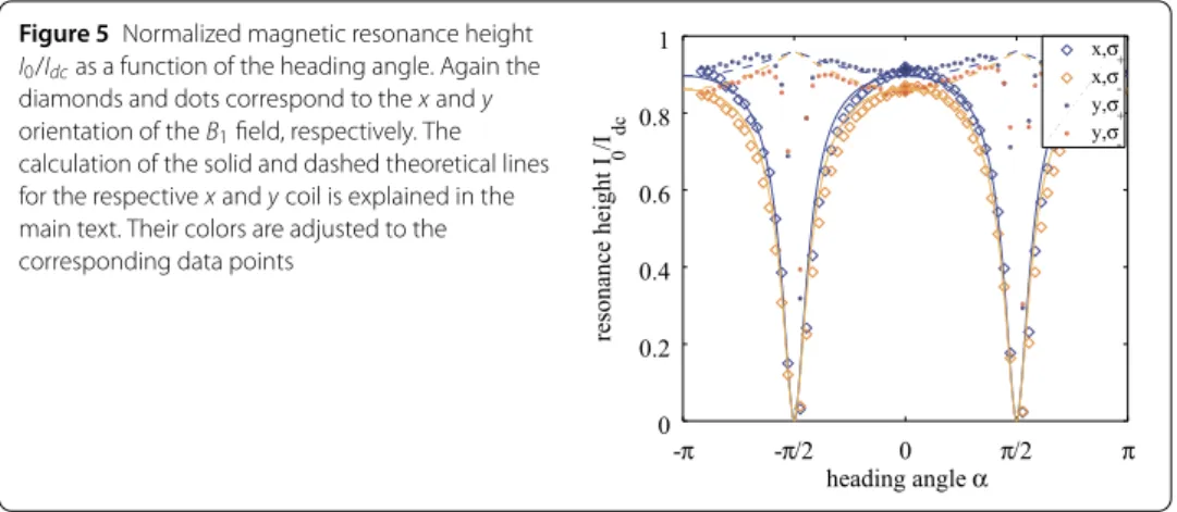
3.3 Magnetic resonance amplitude

In contrast to the very similar angular dependencies of the dc-photocurrent for the two diﬀerentB1coils, a clear discrepancy is found in the normalized amplitude of the magnetic

(10)

Figure 5Normalized magnetic resonance height

I0/Idcas a function of the heading angle. Again the diamonds and dots correspond to thexandy

orientation of theB1ﬁeld, respectively. The

calculation of the solid and dashed theoretical lines for the respectivexandycoil is explained in the main text. Their colors are adjusted to the corresponding data points

This mentioned discrepancy is well explained by the additional modiﬁcation of the ef-fectiveB1ﬁeld amplitude when modifying its direction compared toB0. We included this

in our calculation by the factorcthat is constantly 1, when using they-coil, and|cosα|, when thex-coil is used. With Eq. (5) we ﬁt the normalized amplitudes presented in Fig.5

and found very good agreement between experiment and theory with a factorp2= 0.12.

Note, forσ+we additionally had to adjust the value ofp2by a factor of 1.6. The

depen-dence we observed for the normalized resonance amplitude driven by the x-coil is strongly influenced by thecosfunction given for the effectiveB1-field amplitudeΩ. Namely, the

resonance height is maximal at α= 0 andπ and tends to zero in vicinity ofα=±π/2, where eﬀectively noB1ﬁeld remains.

In contrast, when using they-coil, our theory predicts an increase in resonance ampli-tude towards one for angles close toα=±π/2. Except in close vicinity of these angles this general tendency is also found in the experiment. From our model, it is clear that this increase is connected to a reduction of the optical pumping to the dark state: A given strength of theB1-ﬁeld corresponds to a certain rate of population shifting back from the

dark state to absorbing states. In other words, theB1ﬁeld introduces a Rabi oscillation

whose frequency depends on the ﬁeld amplitude. Thus for larger powers, the shifting of population to the absorbing state is faster. If this rate is smaller than the possible popu-lation transfer that can be achieved by the pumping laser, the measured photocurrent in resonance does not reach down to zero. Therefore the amplitudeI0/Idcis smaller than one.

When rotating towards±π/2 and using they-coil, the eﬀectiveB1ﬁeld amplitude stays

constant. Because at the same time the optical pumping to the dark state gets less eﬀective, the photocurrent amplitude is increased towards one. That means that all the atoms that are optically pumped contribute to the resonance with theB1ﬁeld. Still, our model does

not accurately reproduce the extracted values in close vicinity ofα=±π/2, where the ex-perimentally observed amplitudes drop to zero. This deviation probably results from not considering the linearly polarized pumping at these angles, that not only leads to optical alignment but also takes the role of theB1ﬁeld in redistributing population.

3.4 Resonance width

A ﬁtting of the experimentally observed resonance widths with the same parametersp1

andp2turned out to be unsuccessful. Thus we found it necessary to introduce an

addi-tional ﬁtting parameterp3to Eq. (11). Theoretical curves with parametersp3= 3.5 and

(11)

Figure 6FWHM of the magnetic resonances as a function of the angleα. Again diamonds and dots correspond to the use ofxandycoil for applying the rf-ﬁeld, respectively. In green, we added the corresponding diﬀerence betweenσ+andσ–

result. The solid lines correspond to calculation results following Eq. (11) in the same color as the corresponding data points

Our adjusted model again ﬁts nicely to the experimental results in the case of thex-coil as demonstrated by the solid lines’ correspondence to the data presented as diamonds in Fig.6. We observe a reduction of the power broadening introduced by the rf-ﬁeld. There-fore, we assume that close to angles ofα=±π/2 the minimal possible magnetic resonance width is achieved for this certain temperature and laser power.

In contrast, applying a constant eﬀective magnetic rf-ﬁeld by they-coil, leads to a strong increase of the resonance width in the experiment. We account this to a large redistribu-tion of popularedistribu-tion between Zeeman states resulting in an overlay of several ground state transitions and the linear optical pumping remaining at these angles. Since our model is re-stricted to two-levels and we neglected the linear pumping, we fail to catch the magnitude of this increase in magnetic resonance width. Still, we note that the qualitative behavior is accurately reproduced by the theoretical model.

As already mentioned above, we account the factorp3to a power broadening due to the

strong laser power. To justify this assumption we can estimate the expected laser power broadening similar to Eq. (12) by (compare e.g. Ref. [30])

νlaser=

Ω_L2

2ΓϕΓopt

= 3.5, (15)

where we used the values forΩLof theσ+beam andΓoptas noted above. Since this value

is in agreement with the ﬁtting parameter, we identify the strong power of the detuned laser as one important source of broadening of the magnetic resonance.

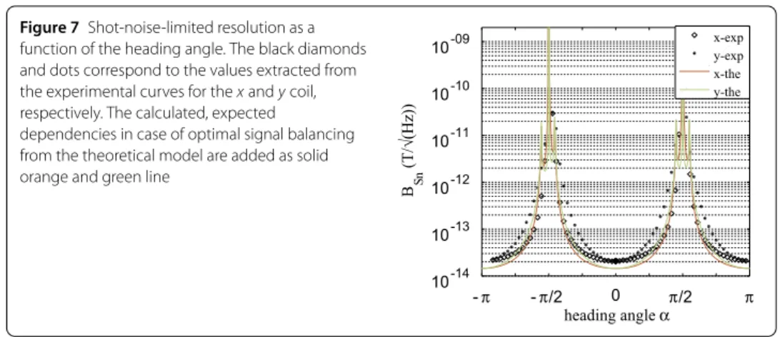
3.5 Shot-noise-limited sensitivity

(12)

Figure 7Shot-noise-limited resolution as a function of the heading angle. The black diamonds and dots correspond to the values extracted from the experimental curves for thexandycoil, respectively. The calculated, expected

dependencies in case of optimal signal balancing from the theoretical model are added as solid orange and green line

both the magnetic resonance signal as well as the light shift are reduced resulting in a loss of sensitivity.

We observe a strong dependence of the amplitude and width of the magnetic resonance signals on the angle that additionally is slightly diﬀerent for the two used orientations of theB1coils. Still, because the width of the magnetic resonance as well as the light shift are

both dominated by the laser intensity, the shot noise limited resolution is quite stable for angles of±20◦around optimal orientation.

As shown above, our model allows for a description of the orientation dependence of all the key parameters of the magnetic resonance. Thus it enables us to estimate the shot noise limited sensitivity as a function ofαin the case of perfect balancing of the channels. To do so, we calculate the steepness of a single resonance curve as the derivative of (1)

s

2=

_ddI_ν= 8I0ν

2₍_ν_–_ν 0)

(4(ν–ν0)2+ν2)2

(16)

and evaluate it at ν=ν0 +νLS. There the maximal steepness of the LSD-Mz signal is

achieved and corresponds to twice the value of a single magnetic resonances(ν0+νLS) =

2|_ddI_ν|(ν0+νLS). Substituting into the equation for the shot-noise-limited resolution (2)

re-sults in

Bsn=

e Idc

1 8γi0

(4ν_LS2 +ν2)2

ν2_ν

LS

, (17)

with the parametersIdc,i0, andνdeﬁned by the respective equations (8), (10), and (11).

The theoretical estimated sensitivity is added to Fig.7. In the calculation we used the ex-perimental parameters of the starting angle and forσ+light and assumed perfect channel

balancing. In general a slightly better sensitivity is expected from our calculation but the qualitative shape ﬁts very well to the experiment. Note, the two additional peaks around angles of ±π/2 result from the overlay of the two resonance curves for theσ± beams

meaningωLS= 0, as can be seen in the plotted resonance frequencies of Fig.3. This

(13)

4 Discussion of results and conclusion

We experimentally analyzed the performance of an OPM operated in the LSD-Mz mode at Earth magnetic field strengths as a function of the heading of the sensor. We found that the reconstructed Larmor frequency for all heading angles corresponds accurately to the magnetic field when the two channels with different helicities are well balanced. The shot noise limited resolution strongly depends on the orientation in the external magnetic field. We demonstrated that this is related to the modified atom-light coupling responsible for both, a reduction of the photocurrent due to a reduction of spin polarization and a smaller light shift. The strong optical pumping leads to a strong contribution of power broadening to the magnetic resonance widths. This is added to the power broadening induced by the

B1ﬁeld. The orientation of the latter has a strong inﬂuence to the amplitude and width of

the resonance signal. Nevertheless, in terms of shot noise limited resolution the two coils produce similar dependencies on the orientation angle.

Our experimental results can be explained in frame of light-shift calculations and Bloch equations. It was necessary to include the modiﬁed optical pumping into the latter by introducing heading dependent relaxation and excitation rates to a two-level model. This allows us to qualitatively and to a large extent also quantitatively describe our experimental results. We note, that such a model is not restricted to the description of the LSD-Mz mode, discussed in this work.

Finally, we conclude that a sensor operated in the LSD-Mz regime should be roughly

±20◦ aligned to the direction of the measured magnetic field vector to achieve a good field sensitivity. Notably, for well balanced beams the actual error in the Larmor frequency induced by light shift to each individual magnetic resonance is canceled by their subtrac-tion. That gives a reasonable flexibility in adjusting the heading of an OPM sensor in an external magnetic field which allows their operation in Earth field strengths.

Acknowledgements

We acknowledge the support of the clean room staﬀ under supervision of U. Hübner at the Competence Center Micro-and Nanotechnologies of the Leibniz IPHT in the fabrication of the cesium vapor cell used in the experiment.

Funding

The authors acknowledge the financial support by the Federal Ministry of Education and Research (BMBF) of Germany under Grant No. 033R130E (DESMEX). The project 2017 FE 9128, funded by the Free State of Thuringia, was co-financed by European Union funds under the European Regional Development Fund (ERDF). This work was conducted using the infrastructure supported by the Free State of Thuringia under Grant No. 2015 FGI 0008 and co-financed by European Union funds under the European Regional Development Fund (ERDF). This work has received funding from the German Research Foundation (DFG) under Grant No. SCHU 2845/2-1; AOBJ 621093. The publication of this article was funded by the Open Access Fund of the Leibniz Association.

List of abbreviations

BS, beam splitter; DP, deﬂecting prism; F, bandpass ﬁlter; FWHM, full width half maximum; HL, heat laser; KL, collimating lens; L, lens; LN, light narrowing; LP, linear polarizer; LSD-Mz, Light-shift dispersedMz; OPM, optically-pumped

magnetometer; PBS, polarizing beam splitter; PD, photo diode; PL, pump laser; rf, radio frequency.

Availability of data and materials

The data generated and analysed during the current study is available from the corresponding author on reasonable request.

Competing interests

The authors declare that they have no competing interests.

Authors’ contributions

RIJ, VS, and RS planned the experiment. RIJ, VS, and GO created the experimental setup and carried out the measurements. GO made the data analysis and theoretical calculations. All authors participated in interpretation of results and writing the manuscript. RS supervised the project. All authors read and approved the ﬁnal manuscript.

Author details

(14)

Publisher’s Note

Springer Nature remains neutral with regard to jurisdictional claims in published maps and institutional aﬃliations.

Received: 18 June 2019 Accepted: 4 December 2019

References

1. Cohen-Tannoudji C, Diu B, Laloe F. Quantum mechanics. Volume I. New York: Wiley; 1977.

2. Leger J-M, Bertrand F, Jager T, Prado ML, Fratter I, Lalaurie J-C. Swarm absolute scalar and vector magnetometer based on helium 4 optical pumping. Proc Chem. 2009;1(1):634–7.https://doi.org/10.1016/j.proche.2009.07.158. 3. Nabighian MN, Grauch VJS, Hansen RO, LaFehr TR, Li Y, Peirce JW, Phillips JD, Ruder ME. 9. Magnetic exploration

methods. In: Geophysics today. Tulsa: Society of Exploration Geophysicists; 2010. p. 183–213.

https://doi.org/10.1190/1.9781560802273.ch9.

4. Korth H, Strohbehn K, Tejada F, Andreou AG, Kitching J, Knappe S, Lehtonen SJ, London SM, Kafel M. Miniature atomic scalar magnetometer for space based on the rubidium isotope 87 rb. J Geophys Res Space Phys.

2016;121(8):7870–80.https://doi.org/10.1002/2016ja022389.

5. Budker D, Kimball DFJ, editors. Optical magnetometry. New York: Cambridge University Press; 2013. 6. Oelsner G, Schultze V, IJsselsteijn R, Wittkämper F, Stolz R. Sources of heading errors in optically pumped

magnetometers operated in the Earth’s magnetic ﬁeld. Phys Rev A. 2019;99(1):013420.

https://doi.org/10.1103/physreva.99.013420.

7. Jensen K, Acosta VM, Higbie J, Ledbetter M, Rochester S, Budker D. Cancellation of nonlinear Zeeman shifts with light shifts. Phys Rev A. 2009;79(2):023406.https://doi.org/10.1103/PhysRevA.79.023406.

8. Bao G, Wickenbrock A, Rochester S, Zhang W, Budker D. Suppression of the nonlinear Zeeman eﬀect and heading error in Earth-ﬁeld-range alkali-vapor magnetometers. Phys Rev Lett. 2018;120(3):033202.

https://doi.org/10.1103/PhysRevLett.120.033202.

9. Hu Q-Q, Freier C, Sun Y, Leykauf B, Schkolnik V, Yang J, Krutzik M, Peters A. Observation of vector and tensor light shifts in rb87 using near-resonant, stimulated Raman spectroscopy. Phys Rev A. 2018;97(1):013424.

https://doi.org/10.1103/physreva.97.013424.

10. Colombo S, Dolgovskiy V, Scholtes T, Gruji´c ZD, Lebedev V, Weis A. Orientational dependence of optically detected magnetic resonance signals in laser-driven atomic magnetometers. Appl Phys B. 2016;123(1):35.

https://doi.org/10.1007/s00340-016-6604-8.

11. Weis A, Bison G, Gruji´c ZD. In: Grosz A, Haji-Sheikh MJ, Mukhopadhyay SC, editors. Magnetic resonance based atomic magnetometers. Cham: Springer; 2017. p. 361–424.https://doi.org/10.1007/978-3-319-34070-8_13.

12. Clarke J, Braginski AI, editors. The SQUID handbook: fundamentals and technology of SQUIDs and SQUID systems. Weinheim: Wiley-VCH; 2004.

13. Schmelz M, Stolz R. In: Grosz A, Haji-Sheikh MJ, Mukhopadhyay SC, editors. Superconducting quantum interference devices (SQUID) magnetometers. Cham: Springer; 2017. p. 279–311.https://doi.org/10.1007/978-3-319-34070-8_13. 14. Stolz R, Zakosarenko VM, Fritzsch L, Oukhanski N, Meyer H-G. Long baseline thin ﬁlm SQUID gradiometers. IEEE Trans

Appl Supercond. 2001;11(1):1257–60.https://doi.org/10.1109/77.919578.

15. Chwala A, Stolz R, IJsselsteijn R, Schultze V, Ukhansky N, Meyer H-G, Schüler T. SQUID gradiometers for archaeometry. Supercond Sci Technol. 2001;14(12):1111–4.https://doi.org/10.1088/0953-2048/14/12/327.

16. Foley CP. In: Clarke J, Braginski AI, editors. SQUID system issues. vol. 7. Weinheim: Wiley-VCH; 2004. p. 251. 17. Stolz R. In: Seidel P, editor. Geophysical exploration. Weinheim: Wiley-VCH; 2015. p. 1020. Chap. 9.3.4.

18. Scholtes T, Schultze V, IJsselsteijn R, Woetzel S, Meyer H-G. Light-narrowed optically pumped m x magnetometer with a miniaturized cs cell. Phys Rev A. 2011;84(4):043416.https://doi.org/10.1103/physreva.84.043416.

19. Guo Y, Wan S, Sun X, Qin J. Compact, high-sensitivity atomic magnetometer utilizing the light-narrowing eﬀect and in-phase excitation. Appl Opt. 2019;58(4):734.https://doi.org/10.1364/ao.58.000734.

20. Fu Y, Liu Y, Yuan J. Light narrowing of cesium magnetic-resonance lines in a radio-frequency atomic magnetometer. AIP Adv. 2019;9(1):015304.https://doi.org/10.1063/1.5043231.

21. Schultze V, Schillig B, IJsselsteijn R, Scholtes T, Woetzel S, Stolz R. An optically pumped magnetometer working in the light-shift dispersed mz mode. Sensors. 2017;17(3):561.https://doi.org/10.3390/s17030561.

22. Woetzel S, Schultze V, IJsselsteijn R, Schulz T, Anders S, Stolz R, Meyer H-G. Microfabricated atomic vapor cell arrays for magnetic ﬁeld measurements. Rev Sci Instrum. 2011;82(3):033111.https://doi.org/10.1063/1.3559304.

23. Schultze V, IJsselsteijn R, Meyer H-G. Noise reduction in optically pumped magnetometer assemblies. Appl Phys B. 2010;100(4):717–24.https://doi.org/10.1007/s00340-010-4084-9.

24. Mathur BS, Tang H, Happer W. Light shifts in the alkali atoms. Phys Rev. 1968;171(1):11–9.

https://doi.org/10.1103/physrev.171.11.

25. Shevchenko SN, Oelsner G, Greenberg YS, Macha P, Karpov DS, Grajcar M, Hübner U, Omelyanchouk AN, Il’ichev E. Ampliﬁcation and attenuation of a probe signal by doubly dressed states. Phys Rev B. 2014;89(18):184504.

https://doi.org/10.1103/physrevb.89.184504.

26. Dréau A, Lesik M, Rondin L, Spinicelli P, Arcizet O, Roch J-F, Jacques V. Avoiding power broadening in optically detected magnetic resonance of single NV defects for enhanced dc magnetic ﬁeld sensitivity. Phys Rev B. 2011;84(19):195204.https://doi.org/10.1103/physrevb.84.195204.

27. Shi Y, Scholtes T, Gruji´c ZD, Lebedev V, Dolgovskiy V, Weis A. Quantitative study of optical pumping in the presence of spin-exchange relaxation. Phys Rev A. 2018;97(1):013419.https://doi.org/10.1103/physreva.97.013419.

28. Oelsner G, Macha P, Astaﬁev OV, Il’ichev E, Grajcar M, Hübner U, Ivanov BI, Neilinger P, Meyer H-G. Dressed-state ampliﬁcation by a single superconducting qubit. Phys Rev Lett. 2013;110(5):053602.

https://doi.org/10.1103/PhysRevLett.110.053602.

29. Steck DA. Cesium D line data.https://steck.us/alkalidata/cesiumnumbers.1.6.pdf.