Performance Evaluation of SFR Scheme in Long-Term Evolution - Advanced
Networks
Abdelali EL BOUCHTI, Abdelkrim HAQIQ
Computer, Networks, Mobility and Modeling laboratory e-NGN Research Ggroup, Africa and Middle East FST, Hassan 1st University, Settat, Morocco {a.elbouchti, ahaqiq}@gmail.com
ABSTRACT: In this paper we focus our studies on LTE, which is a development under 3G technologies Release-8 of the 3GPP Project plan and is considered a baseline and step towards the LTE-Advanced. In orthogonal frequency division multiplexing networks, inter-cell interference results in poor performance, especially universal frequency reuse scheme has already been used. Soft Frequency Reuse (SFR) scheme, one of the most promising inter-cell interference coordination (ICIC) schemes, has been introduced in LTE-Advanced networks. In this paper, we develop an analytical queuing model for the SFR scheme taking into account the features of SFR scheme and its impact on system performance firstly. Then, we improve the iterative algorithm called successive over-relaxation (SOR) to solve the set of linear equations and get the steady state probability distribution. Finally, performance analysis shows that maximum number of resource that cell-edge users can use and the number of cell-edge users correlate with the performance of SFR scheme.
Keywords: LTE-Advanced, SFR, Queuing, MMPP, Quality of Service, Performance Evaluation
Received: 10 January 2014, Revised 29 March 2014, Accepted 5 May 2014
© 2014 DLINE. All Rights Reserved
1. Introduction
3rd Generation Partnership Project (3GPP) is currently in the process of defining Long - Term Evolution (LTE) of 3G, which is
considered as the bridge of IMT-2000 system and IMT-Advanced system. In order to improve the LTE system performance in the form of higher bit-rates, lower latencies and a wider array of service offerings, new challenges need to be overcome. A case in point is the issue of the user equipment (UE) power saving, which is an important problem for wireless data transmission since the data bandwidth is significantly limited by the battery capacity [1, 2].
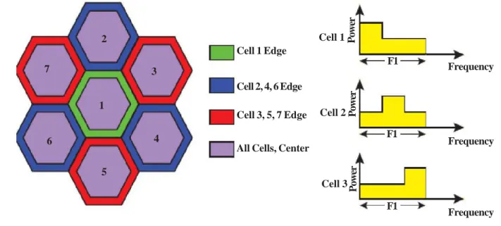
There are three main approaches to mitigate ICI, including inter-cell interference randomization, inter-cell interference cancellation and inter-cell interference coordination (ICIC). Considering the performance and the complexity of ICI mitigation schemes, ICIC is considered as the most promising proposal in 4G networks [1]. Recently, some ICIC proposals from Ericsson [2], Siemens [3], Alcatel [4] and Huawei [5] have already been discussed in 3GPP WG1 meeting. Among them, Soft Frequency Reuse (SFR) scheme from Huawei is accepted as an important technical report. From results in reference [5], the smaller FRF corresponds to more available RBs for each cell and lower Signal to Interference plus Noise Ratio (SINR) due to ICI. On the contrary, larger FRF corresponds to less available RBs and higher SINR. To improve the mechanism that eliminate ICI and increase SINR at the cost of spectrum efficiency aforesaid, The SFR scheme divides the available RBs into two parts: cell-edge RBs and cell-center RBs. All of users within each cell are also divided into two groups which based on the SINR: cell-edge users and cell-center users. Mentality of designing SFR scheme can be seen from Figure 1. Cell-edge users are confined to cell-edge RBs while cell-center users can be access to the cell-center RBs and can also be access to the cell-edge RBs but with less priority than cell-edge users. It means that cell-center users can use cell-edge RBs only when there are remaining available cell-edge RBs.
Naturally, the shortcomings of SFR scheme bring enthusiasm to improve it from different aspects. X.Zhang has suggested an improved SFR scheme named Softer Frequency Reuse (SerFR) scheme [6]. In SerFR scheme, the cell-edge users have access to all of RBs by using proportional fairness scheduling algorithm to increasing the cell-edge user’s throughput. X.Mao has proposed Cell-edge Bandwidth Breathing Scheme (CEBS) that simply control the allocation of the cell-edge RBs by referring to the each cell traffic load [7]. Considering multi-service requirement, W.Wang has developed SFR scheme at the point of QoS and distribution [8].
No one resolves the essential problem that ICI results in the shortage of system resource. One of the mathematical models called queuing model [17] can be able to reflect utilization of system resource efficiently. A useful queuing model both represents a real-life system with sufficient accuracy and is analytically tractable. In this paper, we first propose a proper queuing model to analyze the soft frequency reuse scheme and the impact due to ICI. Then, an improved iterative algorithm is used to solve the set of linear equations and acquire the steady state probability distribution. Finally, we successfully prove that the number of celledge RBs can be used to adjusting the performance of SFR scheme, so does the number of cell-edge users.
The remainder of this paper is outlined as follows. In section 2, we present system model for SFR scheme and performance formulations. Combined with features of queue model of the SFR scheme, we use an improved iterative algorithm to get the steady state probability in section 3. Analytical results and analysis are presented in section 4 and concluding remarks are drawn in section 5.
Figure 1. Schematic diagram of various traffic channel ICIC solutions, showing ICIC in frequency domain (left) and ICIC in frequency and power domains (right)
Cell 1 Edge
Cell 2, 4, 6 Edge
Cell 3, 5, 7 Edge
All Cells, Center 1
2
7 3
4
5 6
Cell 1
Cell 2
Cell 3
Power
Power
Power
F1
F1
F1
Frequency
Frequency
2. Network Architecture
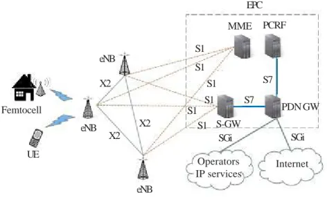
The core network of the Advanced system is separated into many parts. Figure 1 shows how each component in the LTE-Advanced network is connected to one another [12- 14]. NodeB in 3G system was replaced by evolved NodeB (eNB), which is a combination of NodeB and radio network controller (RNC). The eNB communicates with User Equipments (UE’s) and can serve one or several cells at one time. Home eNB (HeNB) is also considered to serve a femtocell that covers a small indoor area. The evolved packet core (EPC) comprises of the following four components. The serving gateway (S-GW) is responsible for routing and forwarding packets between UE’s and packet data network (PDN) and charging.
In addition, it serves as a mobility anchor point for handover. The mobility management entity (MME) manages UE access and mobility, and establishes the bearer path for UE’s. Packet data network gateway (PDN GW) is a gateway to the PDN, and policy and charging rules function (PCRF) manages policy and charging rules.
3. Model Description and Performance Formulation 3.1 Basic Assumption
1) The basic resource element considered in this paper is the Physical Resource Bloc (PRB) which spans both frequency and time dimensions [9]. The scheduler in eNodeB in the cell allocates each PRB only to one user every time.
2) We have not considered improvement in system performance by adjusting the transmission power spectrum density ratio of cell-center region to cell-edge region in this paper, because further discussion has already existed in Huawei’s proposal.
3) We set α as the ratio of cell-edge PRBs to the total number of PRBs each cell. Let N denote the total number in a cell. Cell-edge users can use the maximum number of PRBs with L = α N called cell-edge PRBs. We introduce another equation that
means cell-center users can use the minimum number of PRBs with (1) M = (1 − α) N called cell-center PRBs.
4) We model the arrival process of new calls to the network as a Markov Modulated Poisson Process (MMPP). The arrival rate of calls into the network is governed by an underlying Markov chain such that when this Markov chain is in state s, new calls arrive into cell i according to a Poisson process with rate λij . The holding time of a call arriving in cell i is exponential with rate
Figure 2. LTE-Advanced network architecture
1
µi(i = e (edge) or i = c (center))
The MMPP allow us to capture correlation between arrivals into a single cell, and in the case of a multi-cell network, to capture correlation in space, that is correlation between arrivals to different cells, as well.
eNB eNB
eNB
UE
SGi SGi
EPC
PCRF MME
S-GW
PDN GW Femtocell
X2 X2
X2 S7
S7 S1
S1
S1
S1 S1
S1
Operators
5) Users are distributed uniformly in a cell. A new call follows an MMPP process. In last section, we divide users into cell-edge users and cell-center users by SINR. The distance between users to eNodeB in a cell is the only determining factor to SINR when we have not considered shadow loss and the fast fading loss. The target cell can be modeled by two queues with the mean arrival rates in state s λc, s = βc λs and λe, s = βe λs , respectively βc represents the ratio of cell center area to the whole cell area, while βe represents the ratio of cell-edge area to the whole cell area.
6) A cell-edge user may be blocked or denied access if there are no available cell-edge PRBs in target cell. A there are no more cell-center PRBs or cell-edge PRBs in target cell. System may force the cell-center call which has already connected to the networks to be terminated if the cell-center call has occupied cell-edge PRBs and a new cell-edge user initialized a new call simultaneously.
3.2 Markov Modulated Poisson Process (MMPP)
The Markov-modulated Poisson process (MMPP) has been extensively used for modeling these processes, because it qualitatively models the time-varying arrival rate and captures some of the important correlations between the inter-arrival times while still remaining analytically tractable [11, 12, 13, 14, 15, 16].
The MMPP is the doubly stochastic Poisson process whose arrival rate is given by λ [S (t)], where S(t) = t ≥ 0 , is an S-state irreducible Markov process. Equivalently, a Markov-modulated Poisson process can be constructed by varying the arrival rate of a Poisson process according to an S-state irreducible continuous time Markov chain which is independent of the arrival process. When the Markov chain is in state s, arrivals occur according to a Poisson process of rate λs. The MMPP is parameterized by the S-state continuous-time Markov chain with infinitesimal generator QMMPP and the S Poisson arrival
rates λ1, λ2...., λs We use the notation.
− q1 q12 .... q1S
q21 − q2 .... q2S
qS1 qS2 .... − qs
. . . .
. . . . . . . . . . . .
qi =
Σ
m
j≠i
qij
⎠⎠⎠⎠⎠
⎞⎞⎞⎞⎞
⎛⎛⎛⎛⎛
⎝⎝⎝⎝⎝
In the following, this MMPP is assumed to be homogeneous, i.e., QMMPP and Λ do not depend on the time t. The steady-state vector of the Markov chain is πMMPP such that
πMMPP QMMPP= 0, πMMPP e = 1,
Λ= diag (λ1, λ2...., λs), λ =( λ1, λ2...., λs)T
where e = (1, 1,..., 1)T is the column vector length m.
In the 2-state case πMMPP is given by
πMMPP = (πMMPP, 1, πMMPP, 2) = 1
QMMPP =
(q2, q1) (q1+ q2)
3.3. Mathematical Model
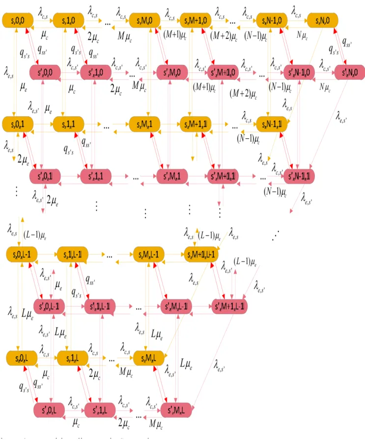
Let S (t) be the underlying Markov chain that governs the arrival rates, with state space (1, 2, …., S). The state of the system is described by the process X (t) = S (t), Nc (t), Ne (t) where Nc (t) is the number of PRBs in cell center at time t and Ne (t) is the number of PRBs in cell edge. The state space of this system is
Ω = {(s, i, j) / 0 ≤ s ≤ S, 0 ≤ i ≤ N, 0 ≤ j ≤ L, i + j ≤ N}
where N is the total number of PRBs in cell center. Such a multidimensional continuous time Markov chain does not have a product-form solution.
Figure 3. Transition diagram in SFR scheme
Let π (s, i, j ) be the steady state probability distribution for a valid state (s, i, j )∈Ω. On the basis of the transit diagram, we introduce the set of global balance equations as follows (see appendix C).
3.4 Performance formulation
Cell blocking probability and cell outage probability are the most important performance metrics in LTE-Advanced networks. We define Γblcok, c and Γblcok, e as the subsets of states where a new arriving cell-center user and a cell-edge user are blocked, respectively. We also define Γoutage as the subset of states where system forces to terminate the holding call. Then, the cell
blocking probability is calculated as:
Σ
Pblcok =
(s, i, j ) ∈ Γ
β cπ (s, i, j ) +
Σ
(s, i, j ) ∈ Γβ e π (s, i, j )
The cell outage probability is given by:
Poutage =
Σ
(s, i, j ) ∈ Γoutage
blcok, c blcok, e
β eπ (s, i, j )
4. Algorithm implementation
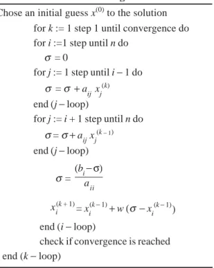
In this section, we design steps to solve the set of linear equations applying an iterative method called successive over-relaxation (SOR) algorithm [10]. In numerical linear algebra, the method of SOR is a variant of the Gauss-seidel method, resulting in fast convergence. Let w denote the relaxation factor to control the speed of convergence. For simplicity but without loss of generality, the service rate of a cell-edge user equals to the service rate of a cell-center user in our study. Before we show the steps in detail, we need to calculate the SOR equations which are a variant of global balance equations first.
4.1 Successive over-relaxation method
Gauss-Seidel method uses updates information immediately and converges more quickly than the Jacobi method. In some large systems of equations the Gauss-Seidel method converges at a very slow rate. Many techniques have been developed in order to improve the convergence of the Gauss-Seidel method. Perhaps one of the simplest and widely used methods is successive over-relaxation (SOR). A useful modification to the Gauss-Seidel method is defined by the iterative scheme.
j = 1 i = 1, 2 , ... k = 1, 2, ...
= (1 − w) xi
xi (k)
+ wa
ii
[ bi +
Σ
i − 1
aij xj(k + 1)+
Σ
nj = i + 1 aij xj(k) (k + 1)
j = 1
i = 1, 2 , ... k = 1, 2, ... = xi
xi (k)+ w
aii[bi +
Σ
i − 1aij xj(k + 1)+
Σ
nj = i + 1 aij xj(k) (k + 1)
The matrix form of the SOR method can be represented by
x(k + 1)=(D + wL)− 1 [(1 − w) D + wU] x (k) + w (D − wL) − 1 b,
which is equivalent to
Tw =(D + wL)− 1 [(1 − w) D +wU ] and c =w (D − wL)− 1 b,
are called the SOR iteration matrix and the vector, respectively.
The quantity w is called the relaxation factor. It can be formally proved that convergence can be obtained for values of w in the large 0 < w < 2. For w = 1 , the SOR method (1) is simply the Gauss-Seidel method. The methods involving (1) are called relaxation methods. For choices the 0 < w < 1, the procedures are called under-relaxation methods and can be used to obtain or, it can be written as
]
]
x(k + 1) = Twx (k) + c
where
(1)
(2)
Successive over-relaxation algorithm Chose an initial guess x(0) to the solution
for k := 1 step 1 until convergence do for i :=1 step until n do
σ = 0
for j := 1 step until i − 1 do
σ = σ + aij xj(k)
end (j − loop)
for j := i + 1 step until n do
σ = σ + aij xj(k − 1)
end (j − loop)
end (i − loop)
check if convergence is reached end (k − loop)
σ = (bi − σ)a
ii
= xi + w (σ − xi xi(k + 1) (k − 1) (k − 1)
)
the convergence of some systems that are not convergent by the Gauss-Seidel method. For choices 1<w < 2, the procedures are called over-relaxation methods, which can be used to accelerate the convergence for systems that are convergent by the Gauss-Seidel method. The SOR methods are particularly useful for solving linear systems that occur in the numerical solutions of certain partial differential equations.
4.2 SOR Algorithm Equations
We need to calculate the following equations in sequence, because current system states transmit from former system states.
5. Numerical Analysis
Using Matlab software, we evaluate and display the performance of SFR scheme via our queuing model. We take seven-cell hexagonal layout with omnidirectional antennas at the center of each cell. There are 48 available PRBs in each cell (denoted by
N = 48). Let alpha denote the ratio of cell-edge PRBs to the total number of PRBs each cell as α. Let beta denote the ratio of
cell-edge area to the whole cell area as βeaforesaid. A holding user follows an Exponent distribution with the mean service period of 90 seconds.
5.1 Impact of Arrival rate and Beta on Performance Metrics
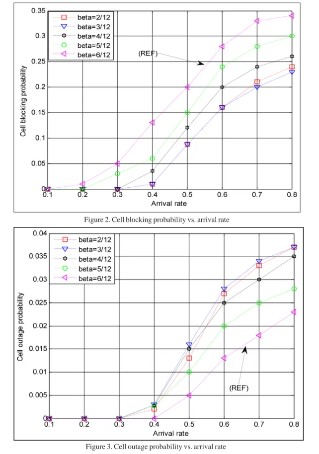
Figure 2 shows the cell blocking probability for different beta considered in this paper when alpha = 4/12 = 1/3. It is observed that cell blocking probability for each beta increases as arrive rate of calls increases. With a higher arrival rate of calls; more calls will be blocked because of shortage of valid PRBs in the cell. It is necessary to take Huawei’s proposal as reference, where one-third of total PRBs is allocated to the cell-edge users (denoted by alpha = 1/3) and cell-edge area is half of the whole cell area (denoted by beta = 1/2). The arrival rate of cell edge users is equal to the arrival rate of cell center users when beta = 1/2. As a consequent, cell blocking probability when beta = 6/12 = 1/2 is higher than the probability when beta = 5/12, 4/12, 3/ 12 and 2/12 from Figure 2. We can also discover that the difficulty of improving the cell blocking probability arises as beta decreases until the improvement can not be made.
be found with further discussion.
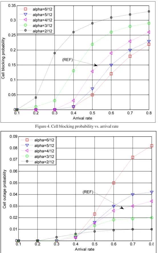
5.2 Impact of arrival rate and alpha on performance metrics
Figure 4 shows the cell blocking probability for different alpha considered in this paper when beta = 1/3. We can discover that
Figure 2. Cell blocking probability vs. arrival rate
Figure 4. Cell blocking probability vs. arrival rate
Figure 5. Cell outage probability vs. arrival rate
6. Conclusion
In this paper, we have investigated Soft Frequency Reuse (SFR) scheme in forthcoming cellular system called LTE-Advanced networks. First, we have derived the performance metrics (cell blocking probability and cell outage probability) using queuing model. Then we devise the iterative algorithm to calculate the set of global balance equations and acquire the proper steady states probability distribution. Finally, our analytical results for SFR scheme shows that we can modify the performance of LTE-Advanced networks by adjusting the maximum number of resource that edge users can use and the number of cell-edge users.
Appendix A
We introduce the set of global balance equations as follows:
For s, s' = 1,…, S, we have:
For i = 0 and j = 0
(λe, s+ λc, s+qss') π (s, 0, 0) + (qs's π (s', 0, 0) + µc π (s, 1, 0) + µe π (s, 0, 1) (A.1)
For i = 0 and j = L
(Lµe+ λc, s+qss') π (s, 0, L) = (qs's π (s', 0, L) + µcπ (s, 1, L) + λe, s π (s, 0, L − 1) (A.2)
For i = M and j = L
(Lµe+Lµc+ qss') π (s, M, L) = (qs's π (s', M, L) +λe, s(π (s, M, L − 1) +π (s, M +1, L − 1)) + λc, sπ (s, M − 1, L ) (A.3)
For i = N and j = 0
(Nµc +qss') π (s, N, 0) = (qs's π (s', N, 0) + λc, sπ (s, N, −1, 0) + λe, s π (s, N, 0) (A.4)
For 0 ≤ i < N ; j = 0
(iµc + λe, s+ λc, s+ qss') π (s, i, 0) = (qs's π (s', i, 0) + (i +1)µcπ (s, i + 1, 0) + µeπ (s, i, 1) + λc, s π (s, i, −1, 0) (A.5)
For i = 0; 1≤ j < L
(jµe+ λe, s+ λc, s+ qss') π (s, 0, j) = (qs'sπ (s', 0, j) + (j +1) µeπ (s, 0, j + 1) + µcπ (s, 1, j) + λe, s π (s, 0, j − 1) (A.6)
For 1≤ i < M; j =L
(Lµe + λc, s+ iµc+ qss') π (s, i, L) = qs's π (s', i, L) + (i +1) µcπ(s, i +1, L) + µeπ(s, i, L − 1) +λc, s π (s, i − 1, L) (A.7)
For M < i < N; i + j =N
(jµe+λe, s+ iµc+ qss') π(s, i, j) = (qs's π(s', i, j) + λc, s π (s, i − 1, j) +λe, s ( π (s, i +1, j − 1) + π (s, i, j − 1)) (A.8)
For 1 ≤ i < N; 1 ≤ j < L, i + j < N
(jµe + λe, s+ λc, s+ iµc + qss') π (s, i, j) = (qs's π (s',i, j) + λc, s π (s, i − 1, L) + λe, sπ (s, i, j − 1) + (j +1) µeπ (s, i, j +1) + (i +1)
µcπ (s, i, +1, j) (A.9)
In addition, the summation of all steady state probabilities satisfies the normalization constraint, such that
Σ
s, i, j ∈ Ω
π (s, i, j) = 1 Appendix B
We introduce the set of global balance equations as follows:
For s, s'= 1,…, S, we have:
For i = 0 and j = 0
π k(
s, 0, 0) = (1 − w) π k − 1 (s, 0, 0) + w
(λe, s+ λc, s+ qss')
[qs'sπ k − 1 (s', 0, 0) +µ
c π k − 1 (
s, 1, 0) +µeπ k − 1(s, 0, 1)]
For i = 0 and j = L
π k (
s, 0, L) = (1 − w) π k − 1 (s, 0, L) + w
(Lµe+ λc, s+qss')[qs'sπ
k − 1 (s', 0, L) +µ
c k − 1 (
s, 1, L) + λe, sπ k(s, 0, L − 1)]
For i = M and j = L
π k (
s, M, L) = (1 − w) π k − 1 (s, M, L) + w
(L(µe+ µc+qss') [qs'sπ
k − 1 (s', M, L) +λ
c, sπ
k(
s, M− 1, L) + λe, sπ k (s, M, L − 1) +
For i = N and j = 0
π k
(s, N, 0) = (1 − w) π k − 1(s, N, 0) + w
(Nµc + λe, s+qss')[qs'sπ k − 1 (
s', N, 0) +λc, sπ k (s, N− 1, 0)]
For state 1 ≤ i < N ; j = 0
πk(
s, i, 0) = (1 − w) π k − 1(s, i, 0) + w
(iµc + λe, s+ qss')
+ π k (s, M+ 1, L − 1)]
For state i = 0; 1 ≤ j < L
πk(
s, 0, j) = (1 − w) π k − 1(s, 0, j) + w
(jµe+ λe, s+λc, s+qss')
[qs'sπ k − 1 (s', i, 0) +(i + 1) µ
cπ
k − 1 (
s, i + 1, 0) + µeπk −1(s, i, 1) +
[qs'sπ k − 1 (s', 0, j) +(j + 1) µ
e π
k − 1 (s, 0, j + 1, ) + µ
c π k −1(
s, 1, j)
For state 1 ≤ i < M ; j = L
π k(
s, i, L) = (1 − w) π k − 1(s, i, L) + w
(Lµe + λc, s+ iµc+ qss')[qs'sπ
k − 1 (s', i, L) + (i + 1) µ
c π
k − 1 (s, i+ 1, , L ) +λ
e, s π
k (s, i, L − 1) (B.1)
` (B.2)
For state M ≤ i < N ; j = N
π k(
s, i, j) = (1 − w) πk − 1(s, i, j) + w
(Jµe+ λe, s+ iµc+ qss') [qs'sπ
k − 1 (s', i, j) + λ
c, sπ
k (
s, i − 1, j) +λe. s π k (s, i + 1, j− 1 )
For 1 ≤ i < Ν ; 1 ≤ j < L ;i + j < N
π k (
s, i, j) = (1 − w) π k − 1(s, i, j) + w
(Jµe + λe, s+λc, s+iµc+ qss')[qs'sπ k − 1 (
s', i, j) + λc, s π k (s, i − 1, j) +λe. s π k (s, i , j− 1 ) (j+1)+
To simplify,
For s, s' =1,…, S, we have:
For i = 0 and j = 0
πk (
s, 0, 0) = (1 − w) π k − 1(s, 0, 0) + w
(λs +qss')
[qs'sπ k − 1 (s, 0, 0) + µ (π k − 1(s, 1, 0) + π k − 1 (s, 0, 1))]
For i = 0 and j =L
π k(
s, 0, L) = (1 − w) π k − 1(s, 0, L) + w
(Lµ + βc λs + qss')[qs'sπ k − 1
(s’, 0, L) + µ π k − 1 (s, 1, L) + βeλsπ k(s, 0, L − 1)]
λc, sπ k (
s, i− 1, 0)]
+ λe, sπ k(s, 0, j− 1,)]
+ λc, sπ k (s, i − 1, L)]
+π k (s, i, j − 1 )]
µeπ k − 1(
s, i, j+ 1) +(i+1) µcπ k − 1 (s, i + 1, j ) ]
For i = M and j = L
` (B.3)
` (B.4)
` (B.5)
` (B.6)
` (B.7)
` (B.8)
` (B.9)
` (B.10)
πk (
s, M, L) = (1 − w) π k − 1(s, M, L) + w
(2Lµ + qss')[
qs'sπ k − 1 (s', M, L) + β
c λsπ k (
s, M − 1, L) + βe λsπ k (s, M, L − 1)+
For i = N and j = 0
π k (
s, N, 0) = (1 − w) π k − 1 (s, N, 0) + w
(Nµ + βe λs + qss')[qs'sπ k − 1 (
s', N, 0) + βcλsπ k (s, N − 1, 0)]
For 0 ≤ i < N ; j = 0
(iµ + λs + qss')
π k (
s, i, 0) = (1 − w) π k − 1(s, i, 0) + w [qs'sπ k − 1 (s', i, 0) + µ (i + 1) π k − 1(s, i + 1, 0) + µ π k − 1(s, i, 1) +
For i = 0; 0 ≤ j < L
(jµ + λs + qss')
π k (
s, 0, j) = (1 − w) π k − 1(s, 0, j) + w [qs'sπ
k − 1 (s', 0, j) + µ (j + 1)π k − 1(s, 0, j + 1) + π k − 1(s, 1, j) +
For 1 ≤ i < M; j = L
π k(
s, i, L) = (1 − w) πk − 1(s, i, L)+ w
(i + L)µ+ βc λs+ qss') [qs'sπ k − 1 (
s', i, L) + µ (i + 1)π k − 1(s, i + 1, L) +
For M <i < N; i + j = N
πk(
s, i, j) = (1 − w) π k − 1(s, i, j) + w
(Nµ + βe λs+ qss')[qs'sπ
k − 1(
s', i, j) + βc λsπ k (s, i − 1, j) + βeλsπ k (s, i + 1, j − 1) +
For 1 ≤ i < N; 1 ≤ j < L; i + j = N
π k(
s, i, j) = (1 − w) π k − 1(s, i, j) + w
(i + j)µ+ λs+ qss')[qs'sπ k − 1 (
s', i, j) + βc λsπ k (s, i − 1, j) + βeλsπ k (s, i , j − 1) +
References
[1] Boudreau, G., Panicker, J., Guo, N., Wang, N. (2009). Interference Coordination and Cancellation for 4G Networks, IEEE
Tran.Communication.
[2] R1-050763. (2005). Muting-Futher Discussion and Results, Ericsson, 3GPP TSG RAN WG1 Meeting, London, UK, August 28–September 2.
[3] R1-060135. (2006). Interference Mitigation by Partial Frequency Reuse, Siemens, 3GPP TSG RAN WG1 Meeting, Helsinki, Finland, p. 23 – 25 January.
[4] R1-050763. (2005). Multi-cell Simulation Results for Interference Coordination in new OFDM DL, Alcatel, 3GPP TSG RAN WG1 Meeting, London, UK, August 28 – September 2.
[5] R1-050507. (2005). Soft Frequency Reuse Scheme for UTRAN LTE, Huawei, 3GPP TSG RAN WG1 Meeting, Athens, Greece, p. 9 – 13 May.
[6] Zhang, X., He, C., Jiang, L. (2008). Inter-cell Interference Coordination Based on Softer Frequency Reuse in OFDMA Cellular Systems, IEEE ICNNSP.
[7] Mao, X., Maaref, A., Teo, K. H. (2008). Adaptive Soft Frequency Reuse for Intercell Interference Coordination in SC-FDMA based 3GPP LTE Uplinks, IEEE GLOBECOM.
[8] Wang, W., Xu, L., Zhang, Y. (2009). A Novel Cell-level Resource Allocation Scheme OFDMA System, IEEE ICCMC.
[9] TS36.211 V8.6.0. (2009). Physical Channels and Modulation, 3GPP.
µ ((j + 1) π k − 1(s, i , j + 1) + (i + 1) π k − 1 (s, i + 1, j))] '
π k(
s, M + 1, L − 1)
βe λsπ
k (
s, i, L − 1) + βc λsπ k (s, i − 1, L)]
π k (
s, i , j − 1)]
` (B.12)
` (B.13)
` (B.14)
` (B.15)
` (B.16)
` (B.17)
` (B.18)
βcλsπ
k (
s, i − 1, 0)]
βc λsπ
[10] Zhang, Y., Xiao, Y., Chen, H. H. (2008). Queueing Analysis for OFDM Subcarrier Allocation in Broadband Wireless Multiservice Networks, IEEE Tran.Wireless Communication.
[11] Neuts, M. F. (1981). Matrix Geometric Solution in Stochastic Models – An algorithmic approach, The Johns Hopkins University Press, Baltimore.
[12] El bouchti, A., Haqiq, A. (2011). Comparaison of two Access Mechanisms for Multimedia Flow in High Speed Downlink Packet Access Channel, IJAET, 4 (2) 29-35.