On the Optimization of Load Balancing in Distributed Networks in the Presence of Delay

Distributed Networks in the Presence of Delay

Sagar Dhakal1, Majeed M. Hayat1, Jean Ghanem1, Chaouki T. Abdallah1, Henry J´erez1, John Chiasson2, and J. Douglas Birdwell2

1 _{ECE Dept, University of New Mexico, Albuquerque NM 87131-1356, USA}

{dhakal,hayat,jean,chaouki,hjerez}@ece.unm.edu

2 _{ECE Dept, University of Tennessee, Knoxville TN 37996, USA}

{chiasson,birdwell}@utk.edu

Summary. In large-scale distributed-computing environments, there are a number

of inherent time-delay factors that can seriously alter the expected performance of load-balancing (or scheduling) policies that do not account for such delays. This situation arises, for example, in systems for which each computational element (CE) is connected by means of a shared broadband communication medium. The delays, in addition to being large, fluctuate randomly as a result of uncertainties in the network condition and uncertainty in the size of the loads to be transferred between the CEs. The performance of such distributed systems under any load-balancing policy is therefore stochastic in nature and must be assessed in a probabilistic sense. Moreover, the design of load-balancing policies that best suit such delay-infested environments must also be carried out in a statistical framework. Indeed, it has been observed in recent simulation-based and experimental studies that the delay, especially that corresponding to transferring large loads between CEs, can cause the system to fall into a mode whereby CEs unnecessarily exchange loads back and forth. This results in an undesirable situation where loads continue to be in transit. It has been observed that the notion of limiting the number of balancing instants in scheduling algorithms can be used to customize certain load-balancing policies to random-delay environments. But the effectiveness of this strategy depends on the decision as to when and how often such load-balancing cycles are to be executed. If a system starts from a certain unbalanced state, we would expect that there would be an optimal time at which balancing must be executed so as to minimize the overall completion time of a workload. In particular, the load-balancing instant should be large enough to ensure that all CEs have updated knowledge of the state of the system. Yet, the balancing instant should be soon enough so that the system does not remain in an unbalanced state for an excessively prolonged time whereby allowing some of the CEs to be idle. It has also been noticed that an additional strategy for mitigating the effects of delay in load balancing is to reduce the gain, or strength, of the load-balancing policy. That is, for each overloaded CE, only a fraction of the load to be transferred is actually transferred to other CEs. Thus, in view of these unique phenomena that occur in load balancing in delay-infested networks, optimizing the performance over the inter-balancing times and the

load-balancing gains becomes an important problem. In this Chapter, the performance of a single-instant load-balancing strategy on a distributed physical system is studied both theoretically and experimentally. The experiments are performed on an in-house wireless distributed testbed as well as a Monte-Carlo simulation tool. The theoretical analysis is carried out based on the concept of regeneration in stochastic processes. In particular, a probabilistic analysis of the queuing system which models the distributed system is developed and studied.

1 Introduction

Distributing the total computational load across available processors is re-ferred to as load balancing in the literature. A typical distributed system consists of a cluster of physically or virtually distant and independent compu-tational elements (CEs), which are linked to one another by some communi-cation medium. The workload has to be distributed over all the available CEs in proportion to their processing speed and availability such that the overall work completion time is minimized. In most practical distributed systems, due to the unknown character of the incoming workload, the nodes exhibit non-deterministic run-time performance. Thus, it is advantageous to perform the load balancing periodically during a run-time so that the run-time variability is minimized. This is referred to in the literature as dynamic load balancing

[1]. However, the frequent load balancing requires the periodic communica-tion (and transfer of loads, of course) between the CEs so that the shared knowledge of the load state of the system can be used by individual CEs to judiciously assign an appropriate fraction of the incoming loads to less busy CEs according to some load-balancing policy.

Not surprisingly, the expected performance of this dynamic allocation of the workload among the CEs relies heavily on the time-delay factors of the physical medium. For example, in shared communication medium (such as the Internet or a wireless LAN), there is an inherent delay in the inter-node com-munications and transfer of loads. As a result, each node has dated knowledge of any other node in the system and each receives its share of the load after a delayed instant of time. It has been almost universally observed that the types of delay described above degrade the overall performance [1, 2, 3, 4, 5]. In par-ticular, communication delays may lead to unnecessary transfer of loads and large load-transfer delays may lead to a situation where much time is wasted on transferring loads, back and forth, while certain CEs may be idle during the transfer. In other words, a situation may arise where a fraction of the work load remains trapped in transit.

Many load-balancing policies have been proposed for distributed-system categories. These include local versus global, static versus dynamic, and cen-tralized versus distributed scheduling [1, 2, 3]. Some of the existing approaches consider constant performance of the network while others consider determin-istic communication and transfer delay. In [4] and [5], it is assumed that the

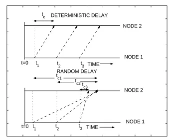
communication channels have fixed delay times and the load balancing is completed within a finite interval. However, in actuality such delays vary ac-cording to the size of the loads to be transferred and also fluctuate due to the random condition of the communication medium that connects the CEs. This introduces the uncertainty in knowledge among the nodes and hence, degrades the performance of any load balancing policy designed for the deterministic delay case. In Fig. 1, a simple comparison is made between the determinis-tic and random communication delay effect on the “knowledge state” of the nodes. In the deterministic case, at any time node 2 receives a communication from node 1, it obtains new information about the queue length of node 1, delayed, however, by a fixed amount of time tc. In contrast, when the delay is random, every time node 2 receives a communication from node 1, there is no guarantee that the received message carries the most recent state of node 1. Similarly, the randomness in the load-transfer delay leads to more uncertainty in the overall completion time. The limitations and the overheads involved with the implementation of the deterministic-delay load-balancing policy in a random delay environment has been discussed previously by the authors [6, 7, 8]. The degraded performance is evident from one of our earlier results, which is presented here in Fig. 2. This result was generated using Monte-Carlo simulation with the assumption that 12000 tasks were initially distributed unevenly among three CEs, each of which can process one task every 10 µs. The communication delay and the transfer delay per task were each set to be uniformly distributed in the intervals (0, 16 ms) and (0, 32ms), respectively. The deterministic-delay load-balancing policy calls for continu-ous execution of the scheduling algorithm. When this policy was applied, the randomness in delay led to an unnecessary exchange of tasks between CEs which results in an undesirable oscillatory behavior near the tail of the queue. Recently, a Monte-Carlo technique [7] was used to investigate a dynamic load balancing scheme for distributed systems which incorporates the stochas-tic nature of the delay in both communication and load transfer. It was shown that indeed there is an interplay between the stochastic delay (e.g., its mean and its dependence on the load) and the strength and frequency of balancing. Moreover, it has been shown that limiting the number of load-balancing in-stants (in an effort to avoid the unnecessary exchange of loads between CEs and reduce communication overhead) while optimizing the strength of the load balancing and the actual load-balancing instants is a feasible solution to the problem of load balancing in a delay-limited environment. It was also observed that by fixing the number of load balancing instants, the performance of the balancing policy becomes very sensitive to the balancing instant (measured relative to the time when load arrives at the system). This is primarily due to the observation that it is more advantageous to balance at a delayed time, up to a point, simply because the CEs will have more time to exchange their respective load states, thereby allowing for “better-informed” load balancing.

t=0 t 1 t2 t3 t=0 t₁ t₂ t 3 TIME NODE 2 NODE 1 TIME NODE 2 NODE 1 t c t_c1 t_c3 t c2 DETERMINISTIC DELAY RANDOM DELAY

Fig. 1. A schematic comparison of the random-delay case with the

deterministic-delay case. The dashed lines represent the communication sent from node 1 to node 2. 0 10 20 30 40 50 60 0 5 10 15 20 25 30 35 40 TIME, ms

Variance in the Queue length

Queue 3

Fig. 2. The variance of the queue size in node 3 (in a three-node system) as a

function of time. High uncertainty in the queue size is evident near the tail. The random delay for transferring small amounts of tasks back and forth causes this oscillation.

One strategy which we have explored is the single-instant load-balancing policy, where upon the arrival of a workload, the load-balancing policy decides on when and how to execute a single load-balancing attempt. This policy has been implemented on a real distributed system consisting of a wireless LAN as well as PlanetLab. In this Chapter, we evaluate the performance of this

policy with respect to the balancing instant and the load-balancing gain pa-rameter. We show that the choice of the balancing strategy is an optimization problem with respect to the balancing instant and the load-balancing gain pa-rameter. We then utilize the delay statistics, obtained from our experiments, to generate the simulations using custom-made Monte Carlo software. The experimental results are compared to the results from the simulation to verify the predictive capability of our model. Finally, an approach for modeling the distributed system dynamics, as a queuing system, is introduced using the concept of regeneration in stochastic processes. We define the events (called regeneration events) whose occurrence will regenerate the queues with simi-lar statistical properties and dynamics. More specifically, on every arrival or departure of a task at any of the nodes, the system of queues is said to be regenerated because they preserve the same stochastic dynamics of the queues prior to this arrival/departure event but will start from different set of ini-tial conditions. The iniini-tial conditions consist of the iniini-tial load of queues as well as their knowledge state of each other. To this end, a novel concept of “information states” of the queues is introduced. We obtain four difference-differential equations which characterize the mean of overall completion time of a two-node system. For brevity, we consider only the zero-input response of the queues, and therefore the arrival of tasks at a node beyond the initial time is solely a result of load transfer from other nodes. Based on this ana-lytical model, we present some initial results showing the optimization of the mean of the overall completion time with respect to the balancing gain. The system model, which is developed here for the special case of two CEs, also maintains the gist of the solution for the multiple-CE problem and conveys the underlying principles of our analytical solution while keeping the algebra at a minimum. The approach, nonetheless, can be extended to the multi-CE case in a straightforward fashion.

This chapter is organized as follows. Section 2 contains the description of the load-balancing policy. The experimental results, on a physical wireless 3-node LAN, are given in Section 3. The simulation results are presented in Section 4 and the stochastic analysis of the distributed system is detailed in Section 5. Conclusions and future extensions are discussed in Section 6.

2 Description of the Load Balancing Policy

We begin by briefly describing the queuing model that characterizes the stochastic dynamics of the load balancing problem described in [6]. Suppose that we have a cluster ofnnodes. LetQ_i(t) denote the number of tasks await-ing processawait-ing at theith node at timet. Assume that theith node completes tasks according to a Poisson process and at a constant rateµi. Let the count-ing process J_i(t₁, t₂) denote the number of external tasks (requests) arriving at node i in the interval [t₁, t₂). (For example, to accommodate the bursty nature of workload arrivals, we can think of J_i(t₁, t₂) as a compound

Pois-son process [9].) The load transfer between nodes is accomplished as follows. The ith node, at the lth specific load-balancing instant ti_l, looks at its own load Q_i(ti_l) and the loads of other nodes (at randomly delayed instants due to communication delays), and decides whether it should allocate a fraction K of its excess load to the other nodes according to a deterministic policy. On the other hand, at the time when it is not attempting to load balance, it may receive loads from the neighboring nodes subject to random delays (due to the load-transfer delays).

We now write the dynamics of the ith queue in a differential form as follows: Q_i(t+∆t) =Q_i(t)−C_i(t, t+∆t)− j=i l L_ji(ti_l)I_[ti l,til+∆t)(t) + j=i k Lij(tj_k)I_[tj k−τij,k,tjk−τij,k+∆t)(t) +Ji(t, t+∆t), (1)

whereI_Ais an indicator function for a setA,C_i(t, t+∆t) is a Poisson process (with rateµi) describing the random number of tasks completed in the interval [t, t +∆t), and τij,k is the delay in transferring load Lij(tj_k) from node j to node i at the kth load balancing instant of node j. More precisely, for k =l, the random loadL_kl(t) diverted from nodel to node k has the form L_kl(t) = g_kl(Q_l(t), Q_k(t−η_lk), . . . , Q_j(t−η_lj), . . .), where for any j = k, η_kj =η_jk is the communication delay between thekth and jth nodes (with the obvious conventionη_ii= 0). The function g_kl dictates the load-balancing policy between thekth andlth nodes. In this chapter, we will use the special form: g_kl(Q_l(t), Q_k(t−η_lk), . . . , Q_j(t−η_lj), . . .) = Kp_kl Q_l(t)−n−1 n j=1 Q_j(t−η_lj)u(t−η_lj) ·u Q_l−n−1 n j=1 Q_j(t−η_lj)u(t−η_lj) , (2)

where u(·) is the unit step function,K is a gain parameter that controls the overall strength of load balancing, andp_kl is the fraction of the excess load at node ito be sent to kth node (_k=lp_kl = 1). Narratively, in this policy the lth node simply compares its load to the average over all load and sends out a fractionpkl of its excess load to thekth node. Finally, the fractionspkl are defined as (assumingn≥3): p_kl=    1 n−2 1−Qk(t−ηlk) i=lQi(t−ηli) , k=l, 1 n−1, otherwise (3)

In this definition, a node sends a larger fraction of its excess load to a node with a small load relative to all other candidate recipient nodes. For the special

case whenn= 2,p_kl= 1, wherek=l. In all the examples considered later in this chapter, only one load-balancing execution is permitted. That is,ti_l=∞, for alll≥2 and all i≥1.

3 Experimental Results

We have developed an in-house wireless testbed to study the effects of the gain parameterK as well as the selection of the load-balancing instant. We would like to highlight the importance of these experiments since, to our knowledge, no previous work has been done in the optimization with respect to the load-balancing instanttbespecially over a wireless network. The details of the system are described below.

3.1 Description of the experiments

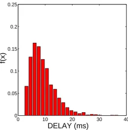
The experiments were conducted over a 802.11b wireless network. The testing was completed on three computers: a 1.6 GHz Pentium IV processor machine (node 1) and two 1 GHz Transmeta Processor machines (nodes 2 & 3). To see the level and variability of the delays over our testbed, we computed the empirical probability density function (pdf) for the wireless-LAN system. The testing was performed by letting the nodes exchange a fixed size frame several times. The empirical pdf was computed and it is shown in Fig. 3. Note the initial almost-zero range, which is dictated by the physical lower bound for the delay, and the approximately exponential decay thereafter.

0 10 20 30 40 0 0.05 0.1 0.15 0.2 0.25 DELAY (ms) f(x)

Fig. 3.Empirical estimate of the probability density function of the delay between

To scale the system to higher delay values proportional to the task exe-cution time, the access point was kept busy by third-party machines, which continuously downloaded files. We consider the case where all nodes execute a single load balancing at a common balancing time t_b.

The application used to illustrate the load-balancing process was matrix multiplication, where one task has been defined as the multiplication of one row by a static matrix duplicated on all nodes (3 nodes in our experiment). The size of the elements in each row was generated randomly from a specified range, which made the execution time of a task variable. On average, the completion time of a task was 525 ms on node 1, and 650 ms on the other two nodes. As for the communication part of the program, UDP was used to exchange queue size information among the nodes and TCP was used to transfer the data or tasks from one machine to another. The load-balancing policy used in the experiments is governed by Eqn. (3), for which the node decides whether or not to utilize either one of the other nodes according to its knowledge state of other nodes.

The aim of the first experiment is to optimize the overall completion time with respect to the balancing instant t_b while fixing the gain value K to 1. Each node was assigned a certain number of tasks according to the following distribution: Node 1 was assigned 60 tasks, node 2 was assigned 30 tasks, and node 3 was assigned 120 tasks. The information exchange delay (viz., commu-nication delay) was on average 850 ms. Several experiments were conducted for each case of the load-balancing instant and the average was calculated us-ing five independent realizations for each selected value of the load-balancus-ing instant. In the second set of experiments, the load-balancing instant was fixed at 1.4 s and the experiments sought to find the optimal gainKthat minimized the overall completion time. The initial distribution of tasks was as follows: 60 tasks were assigned to node 1, 150 tasks were assigned to node 2, and 10 tasks were assigned to node 3. The average information exchange delay was 322 ms and the average data transfer delay per task was 485 ms.

3.2 Discussion of results

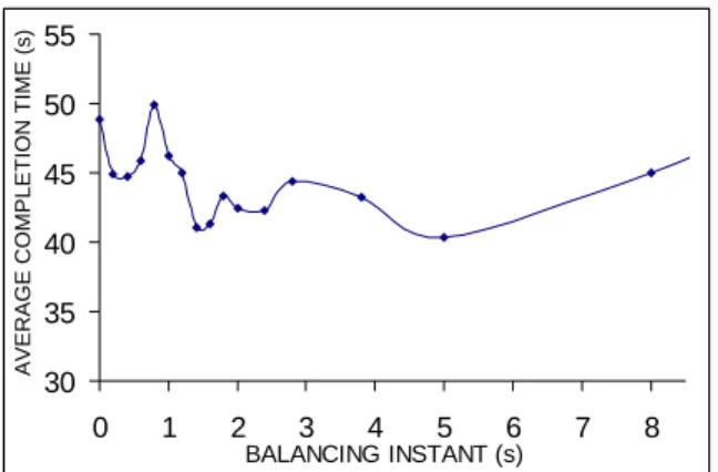
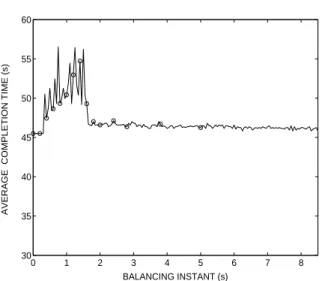
The results of the first set of experiments show that if the load balancing is performed blindly, as in the onset of receiving the initial load, the performance is poorest. This is demonstrated by the relatively large average completion time (namely 45 s ∼ 50 s) when the balancing instant is prior to the time when all the communication between the CEs have arrived (namely when t_b is approximately below 1 s), as shown in Fig. 4. Note that the completion time drops significantly (down to 40 s) ast_b begins to approximately exceed the time when all inter-CE communications have arrived (e.g., tb > 1.5 s). In this scenario of tb, the load balancing is done in an informative fashion, that is, the nodes have knowledge of the initial load of every CE. Thus, it is not surprising that the load balancing is more effective than the case the load balancing is performed on the onset of the initial load arrival for which the

CEs have not yet received the state of the other CEs. The explanation for the sudden rise in the completion time for balancing instants between 0.5 s and 1 s is that the knowledge states in the system are “hybrid,” that is, some nodes are aware of the queue sizes of the others while others aren’t. When this hybrid knowledge state is used in the load-balancing policy (Eqn. (3)), the resulting load distribution turns out to be severely uneven across the nodes, which in turn, has an adverse effect on the completion time. Finally, we observe that as t_b increases farther beyond the time all the inter-CE communications arrive (i.e., t_b > 5 s), then the average completion time begins to increase. This occurs precisely because any delay in executing the load balancing beyond the arrival of the inter-CE communications time would enhance the possibility that some CEs will run out of tasks in the period before any transferred load arrives to them. 30 35 40 45 50 55 0 1 2 3 4 5 6 7 8 BALANCING INSTANT (s) A VER AG E CO MPL E TIO N TIME (s )

Fig. 4. Average total task-completion time as a function of the load-balancing

instant. The load-balancing gain parameter is set at K = 1. The dots represent the actual experimental values and the solid curve is a best polynomial fit. This convention is used throughout Fig. 7.

Next, we examine the size of the loads transferred as a function of the instant at which the load balancing is executed, as shown in Fig. 5. This behavior shows the dependence of the size of the total load transferred on the “knowledge state” of the CEs. It is clear from the figure that for load-balancing instants up to approximately the time when all CEs have accurate knowledge of each other’s load states, the average size of the load assigned for transfer is unduly large. Clearly, this seemingly “uninformed” load balancing leads to the waste of bandwidth on the interconnected network.

The results of the second set of experiments indeed confirm our earlier prediction (as reported in [7]) that when communication and load-transfer delays are prevalent, the load-balancing gain must be reduced to prevent “overreaction” (sending unnecessary excess load). This behavior is shown in

40 60 80 100 120 140 0 1 2 3 4 5 6 7 8 BALANCING INSTANT (s) T A S KS E XC HAN G E D

Fig. 5. Average total excess load decided by the load-balancing policy to be

trans-ferred (at the load-balancing instant) as a function of the balancing instant. The load-balancing gain parameter is set atK= 1.

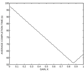
Fig. 6, which demonstrates that the optimal performance is achieved not at the maximal gain (K = 1) but when K is approximately 0.8. This is a sig-nificant result as it is contrary to what we would expect in a situation when the delay is insignificant (as in a fast Ethernet case), where K = 1 yields the optimal performance. Figure 7 shows the dependence of the total load to be transferred as a function of the gain. A large gain (near unity) results in a large load to be transferred, which, in turn, leads to a large load-transfer delay. Thus, large gains increase the likelihood of a node (that may not have been overloaded initially) to complete all its load and remain idle until the transferred load arrives. This would clearly increase the total average task completion time, as confirmed earlier by Fig. 6.

60 70 80 90 100 110 120 0.2 0.4 0.6 0.8 1 GAIN, K AV ERA G E COM P LE TI ON TIME (s)

Fig. 6.Average total task-completion time as a function of the balancing gain. The

0 20 40 60 80 0.2 0.4 0.6 0.8 1 GAIN, K NU M BER O F T ASKS

Fig. 7.Average total excess load to be transferred by the load-balancing policy to

be transferred (at the load-balancing instant) as a function of the balancing gain. The load-balancing instant is fixed at 1.4 s.

4 Simulation Results

We developed generated a Monte-Carlo simulation tool that allows the sim-ulation of the queues described in Section 2 [Eqns. (1) to (3)]. The network parameters (i.e., the statistics of the communication delaysη_kjand the load-transfer delays τ_ij) and the task execution time in the simulation were set according to the respective average values obtained from the experiments de-scribed in Section 3.1. Further, we modeled the load-dependent nature of random transfer delay τ_ij by requiring that its average value,θ_ij =E[τ_ij], be a function ofL_ij according to the following transformation

θij =dmin−1 + exp([(Lijdβ)] −1₎

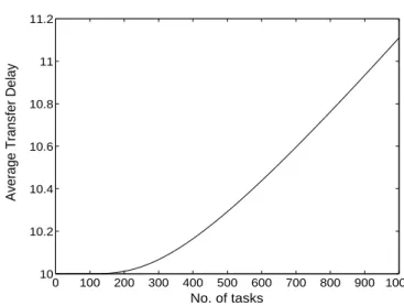
1−exp([(L_ijdβ)]−1), (4) whered_minis the minimum possible transfer delay, anddandβare fitting pa-rameters. This simple, ad-hoc delay model assumes that up to some threshold load, the average delay is d_min, which is independent of the load size. (This minimum delay is dependent, however, on the architecture of the communi-cation medium and we will not be concerned with this dependence in this work.) Beyond this threshold, however, the average delay is expected to in-crease monotonically with the load size. A typical example of the mean of load-dependent transfer delay versus the load is shown in Fig. 8.

For our simulations,dmin was set to be equal to the average value of the transfer delay per task as obtained from the experiments. The parameters d= 0.082618 andb= 0.04955 were selected so that the delay model is in close approximation with the overall average delay for all the actual transfers that occurred in the experiments.

0 100 200 300 400 500 600 700 800 900 1000 10 10.2 10.4 10.6 10.8 11 11.2 No. of tasks

Average Transfer Delay

Fig. 8.Average load-transfer delay as a function of the load size according to (4).

In this example,d= 0.082618 andb= 0.04955.

We used the simulation tool to validate the correspondence between the stochastic queuing model and the experimental setup. In particular, we have generated the simulated versions of Figs. 4, 5 and 6, which are shown below. It is observed that the general characteristics of the simulated curves are very similar to the experiment, but they are not exactly identical, due to the unpre-dictable behavior and complexity of the wireless environment. Nevertheless, the results of the first simulation, shown in Fig. 9, were consistent with the experimental result (shown in Fig. 4) where we can clearly identify the sudden rise in the completion time around the balancing instant corresponding to the communication delay (850 ms). The reason was described in the experimental section. As for the excess transferred load plotted in Fig. 10, the simulation resulted in the same curve and transition shape obtained from the experiment (Fig. 5).

The curve characteristics of the second simulation, shown in Fig. 11, are analogous to the ones obtained in the experiment (Fig. 6). Indeed, the gain values found are almost the same:K= 0.8 from the experiment andK= 0.87 from the simulation. As indicated before, the small difference is due to the unstable delay values and other factors present in the wireless environment which has been approximated both by the model and the simulator.

5 Stochastic Analysis of the Queuing Model: A

Regeneration Approach

Motivated by the fact that we are dealing with a computationally intesive optimization problem, in which we wish to optimize the load-balancing gain

0 1 2 3 4 5 6 7 8 30 35 40 45 50 55 60 BALANCING INSTANT (s)

AVERAGE COMPLETION TIME (s)

Fig. 9.Simulation results for the average total task-completion time as a function

of the load-balancing instant. The load-balancing gain parameter is set atK = 1. The circles represent the actual experimental values.

0 1 2 3 4 5 6 7 8 40 60 80 100 120 140 BALANCING INSTANT (s) TASKS EXCHANGED

Fig. 10. Simulation results for the average total excess load decided by the

load-balancing policy to be transferred (at the load-load-balancing instant) as a function of the balancing instant. The load-balancing gain parameter is set atK = 1. The circles represent the actual experimental values.

and the balancing instants to minimize the average completion time, we have developed a novel regenerative approach that will facilitate the analysis of the queuing model described in Section 2. The concept of regeneration has proven to be a powerful tool in the analysis of complex stochastic systems [9, 10, 11].

0 0.1 0.2 0.3 0.4 0.5 0.6 0.7 0.8 0.9 1 55 60 65 70 75 80 85 90 95 100 GAIN, K

AVERAGE COMPLETION TIME (s)

Fig. 11.Simulation results for the average total task-completion time as a function

of the balancing gain. The load-balancing instant is fixed at 1.4 s.

5.1 Rationale

The idea of our approach is to define an initial event, defined as the comple-tion of a task by any node or the arrival of a communicacomple-tion by any node, and analyzing the queues that emerge immediately after the occurrence of the initial event. We assume that initially all queues have zero knowledge about the state of the other queues. The point here is that immediately after the oc-currence of the initial event, we will have a set of new queues whose stochastic dynamics are identical to the original queues. However, there will be a differ-ent set of initial conditions (i.e., differdiffer-ent initial load distribution if the initial event is a task completion) or different knowledge state (if the initial event happens to be a communication arrival rather than a task completion). Thus, in addition to having an initial load state, we introduce the novel concept of knowledge states (which we informally referred to in previous sections) to be defined next.

In a system of n nodes, any node will receive n−1 number of commu-nications, one from each of the other nodes. Depending upon the choice of the balancing instant, a node may receive all of those communication or may receive none by the time balancing is done. We assign a vector of sizen−1 to each of the nodes and initially set all its elements to 0 (corresponding to the null knowledge state). If a communication arrives from any of the node, the bit position corresponding to that particular node is set to 1. There will be a total of 2n(n−1) number of knowledge states. In the case when two nodes are present, the knowledge states are: 1) state (0,0), corresponding to the case when the nodes do not know about each others initial load; 2) state (1,1), when both nodes know about each other’s initial load states; 3) (1,0),

cor-responding to the case when only node 1 knows about node 2; and 4) state (0,1), which is the opposite of the (1,0) case.

5.2 Regenerative equations

To simplify the description, we consider the case where only two nodes are present. We will assume that each node has an exponential service time with parameters λD1and λD2, respectively. Letmand nbe the initial number of tasks present at nodes 1 and 2, respectively. The communication delays from node 1 to node 2 and from node 2 to node 1 are also assumed to follow an exponential distribution with ratesλ₂₁andλ₁₂, respectively. LetW,X,Y and Z be the waiting times for the departure of the first task at node 1, departure of the first task at node 2, the arrival of the communication sent from node 1 to node 2 and the arrival of the communication sent from 2 to 1, respectively. LetT=min(W,X,Y,Z). A straight-forward calculation shows that the pdf of T can be characterized asf_T(t) =λe−λtu(t), whereλ=λ_D1+λ_D2+λ₂₁+λ₁₂.

Letµk1,k2

m,n (tb) be the expected value of the overall completion time given that the balancing is executed at timet_b, where nodes 1 and 2 are assumed to have mandntasks at timet= 0, and the system knowledge state is (k₁, k₂) at time t = 0. Suppose that the initial event happens to be the departure of a task at node 1 at time t = τ, 0 ≤ τ ≤ t_b. At this instant, the system dynamics remain the same except that node 1 will now have m−1 tasks. Thus, the queue has re-emerged (with a different initial load, nonetheless) and the average of the overall completion time is nowτ+µk1,k2

m−1,n(tb−τ). The effect of other possibilities for the initial event are taken into account similarly. However, to calculate this we need to define the completion time for all cases, i.e., the system initially being in any of the four knowledge states. Based on this discussion, we can characterize the average of the completion times for all four cases below, namely, µ0_m,n,0 (t_b), µ0_m,n,1 (t_b), µ1_m,n,0 (t_b) and µ1_m,n,1 (t_b). For example, in the case ofµ0_m,n,0 (t_b) we obtain the following integral equation

µ0_m,n,0 (t_b) = _∞ tb f_T(s)[µ0_m,n,0 (0) +t_b]ds + _tb 0 fT(s)[µ 0,0 m−1,n(tb−s) +s]P{T =W}ds + _tb 0 fT(s)[µ 0,0 m,n−1(tb−s) +s]P{T =X}ds + _tb 0 fT(s)[µ 0,1 m,n(tb−s) +s]P{T =Y}ds + _tb 0 fT(s)[µ 1,0 m,n(tb−s) +s]P{T =Z}ds. (5) In a similar way, recursive equations can be obtained for the queues corre-sponding to other knowledge states. This would yield (not all shown here

for space constraints) similar equations for µ0_m,n,1 (t_b), etc. For example, for µ1_m,n,1 (t_b), we have µ1_m,n,1 (t_b) = _∞ tb f_T(s)[µ1_m,n,1 (0) +t_b]ds + _tb 0 fT(s)[µ 1,1 m−1,n(tb−s) +s]P{T =W}ds + _tb 0 f_T(s)[µ1_m,n,1 ₋₁(t_b−s) +s]P{T =X}ds + _tb 0 fT(s)[µ 1,1 m,n(tb−s) +s]P{T =Y}ds + _tb 0 fT(s)[µ 1,1 m,n(tb−s) +s]P{T =Z}ds. (6) Moreover, simple calculations yield

P{T =W}= λD1 λ , P{T=X}= λD2 λ , P{T =Y}= λ21 λ , P{T =Z}= λ₁₂ λ . (7)

The above integral equations can be further simplified by converting them into differential equations of standard form. For example, by differentiating Eq. (5) with respect tot_b, we obtain

∂µ0_m,n,0 (t_b)

∂t_b =λD1µ 0,0

m−1,n(tb) +λD2µ0m,n,0 −1(tb)

+λ₂₁µ0_m,n,1 (t_b) +λ₁₂µ_m,n1,0 (t_b)−λµ0_m,n,0 (t_b) + 1 (8) and from Eq. (6) we obtain

∂µ1_m,n,1 (t_b)

∂t_b =λD1µ 1,1

m−1,n(tb) +λD2µ1m,n,1 −1(tb)

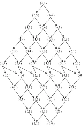
+λ₂₁µ1_m,n,1 (t_b) +λ₁₂µ_m,n1,1 (t_b)−λµ1_m,n,1 (t_b) + 1. (9) Therefore, we arrive at a set of four difference-differential equations which completely defines the queuing dynamics of our distributed system. These equations are coupled with each other in the sense that solving Eqn. (8) re-quiresµ0_m,n,1 (t_b) andµ_m,n1,0 (t_b), each of which in turn requiresµ1_m,n,1 (t_b). Clearly, Eqn. (9) should be solved initially. The recursion involved in this computation is shown in Fig. (12), which is drawn for the casem= 6 andn= 5. The bot-tom of this structure corresponds to the completion time for (m= 0, n= 1) and (m= 1, n= 0) which depend only on λ_D2and λ_D1, respectively. There-fore, we start at the bottom of the structure and move one level upwards to compute completion times for all cases corresponding to that level, until we

( 6,5 ) ( 5,5 ) ( 6,4 ) ( 4,5 ) ( 5,4 ) ( 6,3 ) ( 3,5 ) ( 4,4 ) ( 5,3 ) ( 6,2 ) ( 2,5 ) ( 3,4 ) ( 4,3 ) ( 5,2 ) ( 6,1 ) ( 1,5 ) ( 2,4 ) ( 3,3 ) ( 4,2 ) ( 5,1 ) ( 6,0 ) ( 0,5 ) ( 1,4 ) ( 2,3 ) ( 3,2 ) ( 4,1 ) ( 5,0 ) ( 0,4 ) ( 1,3 ) ( 2,2 ) ( 3,1 ) ( 4,0 ) ( 0,3 ) ( 1,2 ) ( 2,1 ) ( 3,0 ) ( 0,2 ) ( 1,1 ) ( 2,0 ) ( 0,1 ) ( 1,0 )

Fig. 12. Tree for solving Eqn. (9) recursively

finally computeµ1₆,_,1₅(t_b) in this case. It is also intuitively clear that while solv-ing each of these equations, we need to solve for their correspondsolv-ing initial conditions, i.e.,µ0_m,n,0 (0),µ0_m,n,1 (0),µ1_m,n,0 (0) andµ1_m,n,1 (0), which are determined according to the load-balancing algorithm as defined in Section 2. The details of computing the initial conditions are discussed next.

5.3 Initial conditions

Based on the load-balancing policy described in Section 2, we develop a methodology to find µ1_m,n,1 (0), where m ≥ n, using the regeneration princi-ple discussed above. According to Eq. (2), and with p₂₁= 1,L₂₁(0) becomes

L₂₁(0) = floor K(m−n) 2 =L. (10) Case I:L >0

This case corresponds to the scenario for which Ltasks are transferred from node 1 to node 2 at time t = 0, and hence, node 1 has m−L tasks. If T₁

is the waiting time before all of them are served, then the pdf of T₁ can be characterized by the Erlang distribution (since the inter-departure times are independent). More precisely, the distribution function ofT₁ is

F_T1(t₁) = 1− m−L−1 x=0 e−λD1t1(λD1t1)x x! u(t₁). (11)

Justified by the experimental results described earlier, the load-dependent random transfer delayτ₂₁is assumed to follow exponential distribution whose rate,λ_t, is required to be a function ofLaccording to Eqn. (4), whereθ₂₁= 1/λ_t. LetRdenote the number of tasks that are served at node 2 by the time Ltasks arrive, and letT_R denote the waiting time before remaining tasks at node 2 are served. Thus, the total completion time for node 2 isT₂=τ₂₁+T_R. With this decomposition of T₂, we can calculate its probability distribution function as follows: F_T2(t₂) =P{T₂≤t₂} = _∞ −∞P{τ21+TR≤t2|τ21=t}fτ21(t)dt = _∞ −∞ n r=0 P{T_R≤t₂−t|R=r, τ₂₁=t}P{R=r|τ₂₁=t}f_τ21(t)dt. (12) Note that the dependence of T_R on τ₂₁ is through R. Therefore, P{T_R ≤ t₂−t|R=r, τ₂₁=t}=P{T_R≤t₂−t|R=r}, which is given as P{T_R≤t₂−t|R=r}= 1− L+n−r−1 x=0 e−λD2(t2−t)(λD2(t2−t))x x! u(t₂−t). (13)

We also maintain that

P{R=r|τ₂₁=t}= (λD2t)r

r! e−λD2tu(t),0≤r≤n−1. (14) Using Eqns. (12), (13), and (14), we obtain

F_T2(t₂) = 1−e−λtt2−_λ te−λD2t2 _n−1 r=0 L+n−r−1 x=L (λ_D2)r r! (λ_D2)x x! g(t2;r;x) −λ_te−λD2t2 _L−1 x=0 (λD2)x x! g1(t2; 0;x) , (15) where

g(t₂;r;x) = _t2 0 tr(t₂−t)xe−λtt_dt = x k=0 (−1)k x! (x−k)!k!(t2) x−k(r+k)! λr_t+k+1  1−eλtt2 r+k j=0 (λtt2)j j!   g₁(t₂; 0;x) = _t2 0 (t2−t) x_e−(λt−λD2)t_dt

The overall completion time is given as T_C = max(T₁, T₂), and its av-erage E[T_C] is, according to our definition, µ1_m,n,1 (0). Now, by exploiting the independence ofT₁ andT₂, we obtain

µ1_m,n,1 (0) =

_∞

0

t[f_T1(t)F_T2(t) +F_T1(t)f_T2(t)]dt (16)

Case II:L= 0

In this case, no load transfer occurs at all andµ1_m,n,1 (0) can be calculated in a straight-forward manner to yield

µ1_m,n,1 (0) =      m λD1 + n λD2 − (λD1)m (m−1)! _n−1 x=0 (λD1+(mλD+2x))!m+x+1 (λD2)x x! −(λD2)n (n−1)! m−1 x=0 (λD1+(nλ+Dx2))!n+x+1 (λD1)x x! , n >0 m λD1, n= 0 (17) 5.4 Discussion of results

We present an example of the analytical results described earlier for a typical case for which one of the nodes does not have any initial tasks. This not only simplifies our calculations, but also signifies the interplay between the balancing gainK and the balancing instantt_b, and their effect on the overall completion time. Since Eqn. (9) corresponds to the case where m > 0 and n > 0, we will need to develop a new version of it which would handle the special case considered here. Using the principle of regeneration, as described before, µk1,k2

m,0 (tb) can be characterized as a set of four coupled difference-differential equations, each corresponding to a particular initial knowledge state. In the special case considered here, Eq. (9) takes the modified following form ∂µ1_m,,1₀(t_b) ∂t_b =λD1µ 1,1 m−1,0(tb) +λ₂₁µ1_m,,1₀(t_b) +λ₁₂µ_m,1,1₀(t_b)−λµ_m,1,1₀(t_b) + 1, (18) which can be reduced to

∂µ1_m,,1₀(t_b)

∂t_b =−λD1µ 1,1

m,0(tb) +λD1µm1,1−1,0(tb) + 1. (19) Clearly, the communication rate does not play any role here as the initial knowledge state is already (1,1). The solution to Eqn. (19) form≥2 is

µ1_m,,1₀(t_b) = m λ_D1 + m p=2 (λ_D1)m−p−1 (m−p)! [λD1µ 1,1 p,0(0)−p]tbm−pe−λD1tb, (20)

with the obvious fact thatµ1₀,_,1₀(tb) = 0 andµ1₁,_,1₀(tb) =_λ1

D1.

We now present a numerical example. Let node 1 and node 2 each have a service rate given by λ_D1 = 1 task per second. The average load-transfer delay parameters (as defined in Eqn. (4)) are set tod_min= 20 s,d= 0.082618 andβ = 0.04955. The initial load distribution is 200 tasks, which are assigned to node 1; node 2 has no tasks assigned to it. It is observed that for any given value of balancing gain K, the optimal balancing instant is found to be at t_b= 0. Therefore, witht_b = 0, optimization overK is performed as depicted in Fig. 13. The optimal average completion time is 120 s and the optimal gain is 0.9. When the service rate of node 2 is made twice as fast as that for node 1, the optimal balancing instant remains same as before but the optimal K turns out to be equal to 1 as shown in Fig. 14. When the service rate of both

0 0.1 0.2 0.3 0.4 0.5 0.6 0.7 0.8 0.9 1 120 130 140 150 160 170 180 190 200 µ 200,0 1,1 (s) GAIN, K

Fig. 13. Average total task-completion time as a function of the balancing gain.

The load-balancing instanttb= 0.

the processors is increased to 4 tasks per second. The optimal balancing gain turns out to be 0.7 and the optimal average completion time is 43 s, which is shown in Fig. 15. Using the same values for all the parameters, the Monte-Carlo simulation tool is used to generate Fig. 16, which is the empirical version

0 0.1 0.2 0.3 0.4 0.5 0.6 0.7 0.8 0.9 1 100 110 120 130 140 150 160 170 180 190 200 GAIN, K µ 200,0 1,1 (s)

Fig. 14. Same as Fig. 13 but here node 2 is twice as fast as node 1.

of the analytical results shown in Fig. 15. The strong resemblance between the analytical and simulations is evident. Finally, in Fig. 17, we setdmin to

0 0.1 0.2 0.3 0.4 0.5 0.6 0.7 0.8 0.9 1 42 43 44 45 46 47 48 49 50 51 52 GAIN, K µ 200,0 1,1 (s)

Fig. 15. Average total task-completion time as a function of the balancing gain.

Each processor has a service rate of 4 tasks per second.

be 30 s and repeat the calculations. The optimal gain in this case is 0, and therefore, it is better not to send any task to node 2 in this case.

With these results, we clearly see that the choice of the optimalK is de-pendent on a number of factors like the processing speed, transfer delay, and

0 0.1 0.2 0.3 0.4 0.5 0.6 0.7 0.8 0.9 1 42 43 44 45 46 47 48 49 50 51 52 GAIN, K µ 200,0 1,1 (s)

Fig. 16. Same as Fig. 15 but generated by MC simulation.

0 0.1 0.2 0.3 0.4 0.5 0.6 0.7 0.8 0.9 1 50 51 52 53 54 55 56 57 µ 200,0 1,1 (s) GAIN, K

Fig. 17. Same as Fig. 15 but with larger transfer delay.

number of initial tasks. Further, the optimal balancing instant in all these cases is found to be att_b= 0 s, which is also predicted by our earlier simula-tion model. Intuitively, when the initial knowledge state is (1,1), delaying the scheduling instant is not going to bring any new information. Therefore, it is more motivating to optimize the average completion time over t_b when the initial knowledge state is not (1,1). Nonetheless, the optimization overK in itself verifies our notion of presenting the load balancing as an optimization problem.

6 Conclusions

We have performed experiments and simulations to investigate the perfor-mance of load-balancing policy that involves redistributing the load of the nodes only once after a large load arrives at the distributed system. Our ex-perimental results (using a wireless LAN) and simulations both indicate that in distributed systems, for which communication and load-transfer delays are tangible, it is best to execute the load balancing after each node receives com-munications from other nodes regarding their load states. In particular, our results indicate that the loss of time in waiting for the inter-node commu-nications to arrive is overcompensated by the informed nature of the load balancing. Moreover, the optimal load-balancing gain turns out to be less than unity, contrary to systems that do not exhibit significant latency. In de-lay infested systems, a moderate balancing gain has the benefit of reduced load-transfer delays, as the fraction of the load to be transferred is reduced. This, in turn, will result in a reduced likelihood of certain nodes becoming idle as soon as they are depleted of their initial load. We have also developed the analytical model to characterize the expected value of the total completion time for a distributed system when a single scheduling is performed. Our pre-liminary results signify the interplay between delay and load-balancing gain and verifies our notion that the load balancing is an optimization problem.

In our future work, we will use our optimal single-time load-balancing strategy to develop an autonomous on-demand (sender initiated) load-balancing scheme. Every node would have its look-up table for the optimal instant of load-balancing and the optimal gain. The look up-table would be generated up-front using our analytical solution to the queuing model which was de-scribed earlier. As each external request arrives at a node, the node will au-tonomously decide whether or not, when, and how to execute a single-instant load-balancing action. There would be no need to synchronize the balancing instants between all the nodes, and therefore, load balancing can be done dynamically. Although the proposed autonomous on-demand load-balancing dynamic balancing strategy may not lead us to the globally optimal solution, we believe that it will offer an effective solution at a reduced implementation complexity.

Acknowledgements

This work is supported by the National Science Foundation under Information Technology Research (ITR) grants No. ANI-0312611 and ANI-0312182. Ad-ditional support was received from the National Science Foundation through grant No. INT-9818312.

References

1. Z. Lan, V. E. Taylor, and G. Bryan, “Dynamic load balancing for adaptive mesh refinement application,” inProc. ICPP’2001, Valencia, Spain, 2001.

2. T. L. Casavant and J. G. Kuhl, “A taxonomy of scheduling in general-purpose distributed computing systems,”IEEE Trans. Software Eng., vol. 14, pp. 141– 154, Feb. 1988.

3. G. Cybenko, “Dynamic load balancing for distributed memory multiprocessors,” IEEE Trans. Parallel and Distributed Computing, vol. 7, pp. 279–301, Oct. 1989. 4. J. D. Birdwell, J. Chisson, Z. Tang, T. Wang, C. T. Abdallah, and M. M. Hayat, “Dynamic time delay models for load balancing. Part I: Deterministic models,” CNRS-NSF workshop: Advances in Control of Time-Delay Systems, Paris, France, pp. 106–114, January 2003.

5. C-C. Hui and S. T. Chanson,“Hydrodynamic load balancing,” IEEE Trans. Parallel and Distributed Systems, vol. 10, Issue 11, Nov. 1999.

6. M. M. Hayat, S. Dhakal, C. T. Abdallah, J. Chisson, and J. D. Birdwell “ Dynamic time delay models for load balancing. Part II: Stochastic analysis of the effect of delay uncertainty, CNRS-NSF Workshop: Advances in Control of Time-Delay Systems, Paris, France, pp. 115–122, January 2003.

7. S. Dhakal, B. S. Paskaleva, M. M. Hayat, E. Schamiloglu, C. T. Abdallah “Dy-namical discrete-time load balancing in distributed systems in the presence of time delays,” Proceedings of theIEEE CDC 2003, pp. 5128–5134, Maui, Hawaii. 8. J. Ghanem, S. Dhakal, M. M. Hayat, H. J´erez, C.T. Abdallah, and J. Chiasson “Load balancing in distributed systems with large time delays: Theory and experiment,”submitted to the IEEE 12th Miditerranean Conference on Control and Automation, MED’04, Izmir, Turkey.

9. D. J. Daley and D. Vere-Jones,An introduction to the theory of point processes. Springer-Verlag, 1988.

10. C. Knessly and C. Tiery,“Two tandem queues with general renewal input I: Dif-fusion approximation and integral representation,”SIAM J. Appl. Math.,vol.59, pp1917-1959, 1999.

11. F. Bacelli and P. Bremaud, ”Elements of queuing theory: Palm-martingale cal-culus and stochastic recurrence”, New York: Springer-Verlag, 1994.