Load balancing using automatically discovered domain knowledge

(1)

Load balancing using

automatically discovered domain

knowledge

Jouke van der Maas

10186883

Bachelor thesis Credits: 18 EC

Bachelor Opleiding Kunstmatige Intelligentie University of Amsterdam

Faculty of Science Science Park 904 1098 XH Amsterdam

Supervisors

dhr. dr. M.W. van Someren J.G.Noordman Informatics Institute NIPO Software

Faculty of Science Grote Bickersstraat 74 University of Amsterdam 1013 KS Amsterdam

Science Park 904 1098 XH Amsterdam

(2)

Abstract

Existing load balancing algorithms require frequent interaction with or between nodes in a system, which is not always easily available. Alternatively, they require information about the incoming requests that is not trivial to determine when performance is a big factor. The load balancing algorithm presented in this paper solves both these problems by relying on request information that is readily available, by deducing knowledge about the domain using a machine learning approach.

1 Introduction

A load balancing system takes incoming web-requests for a web-based application, and distributes them over a number of servers with the aim of minimizing the response time of incoming requests as well as the number of necessary servers. This results in lower response-times, lower operational costs and higher reliability of service.

Existing load balancing algorithms are both client- and server-agnostic: they work equally well for any system. However, many systems have access to domain-specific information that can improve the load-balancer’s output. This information includes application-specific URL’s and services, that although generally available for most modern services, are still specific to the application. It will be demonstrated that there are benefits to using domain-specific knowledge as input to a load balancing algorithm.

This input will be discovered using existing machine learning techniques. The presented algorithm is general purpose, performant under high load and will adapt to changing requirements over time. The effect will be demonstrated on a business application called Nfield by NIPO Software. This system serves many different kinds of requests and is an example of an application that can benefit from the algorithm described in this paper.

1.1 Prior Work

Many prior studies on the topic of load balancing have been performed. Generally, they focus on improving this balance by taking information that is available for any system in the same form. This leads to very generally applicable algorithms, but ignores some of the subtlety that is often found in modern cloud-based applications.

An overview is given by Aruna, Bhanu, and Punithagowri (2013), in which various algorithms are explained and compared. Although some algorithms of the ones described here consider request properties, most of them do not. Besides, even the algorithms that do take it into account, use a very basic approach to estimating the size of requests, and consequently, the effect on the load of the system.

Begum and Prashanth (2013) also give an overview of load balancing algorithms. Here, the algorithms mostly consider the state of the nodes in the system; the servers that will handle the requests. Again ‘dynamic’ systems that use request properties, such as size as parameter are mentioned, but not prevalent.

Doroudi, Hyytiä, and Harchol-Balter (2014) introduce the concept of job value to load balancing algorithms. However, the authors assume the value of a job is known beforehand: they do not describe a way of deriving it. In practice, this leads to a similar system as described by Altman, Ayesta, and Prabhu (2011), where jobs themselves decide which node will handle them based on their own

(4)

knowledge of their size and value. However, this system is more complicated than a centralized load balancer for all requests, both to implement and to maintain. Nodes will have to redirect requests based on specific knowledge of their contents. This will lead to a slowdown of the system on average, since there will be more complicated paths for requests to follow.

Mukhopadhyay, Karthik, and Mazumdar (2015) propose a system in which a small subset of servers is responsible for distributing the load over the others. This system attempts to fix some of the faults mentioned above. However, it comes at a significant cost of complexity. Although the system has been shown to work well, it is designed for very large clusters of servers. This is not applicable at NIPO Software or similar companies, which would rather use a smaller-scale solution.

1.2 Contributions of this study

Existing algorithms assume the size of requests either as a given or an irrelevant variable, while in practice this is not the case. This study will focus on deter-mining the size of a request without parsing it in its entirety. The system will use this prediction to predict the load on each node in the system. This allows it to make better decisions without the need for communication with or between nodes. This allows for a centralized load balancer that is independent of the system it works for.

Restraints are speed, because if the load balancer is slow, it is of no use, and accuracy: the resulting algorithm must perform better than the naive approach. It will be shown that using the load balancer in described in this paper leads to better distributed load, because it can determine the size of requests based on machine learning techniques.

(5)

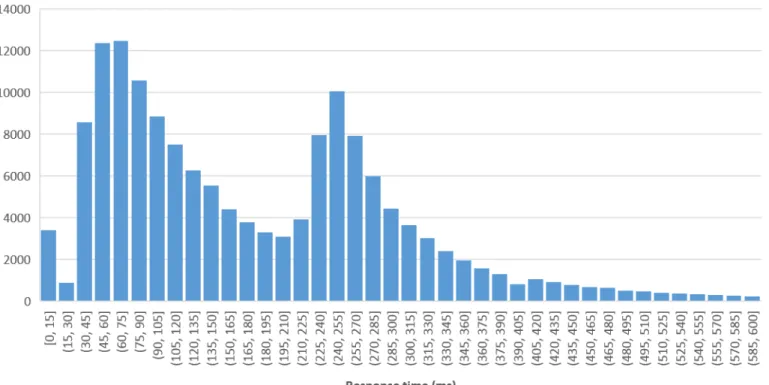
Figure 1: There are clusters in the size-data

2 Approach

The algorithm consists of two components. The first component predicts the response time based on the request (see Section 3.1). The second uses this prediction and uses it to decide which node should handle the incoming data. Because the goal of this paper is just to demonstrate that domain knowledge can improve load balancers’ performance, existing techniques were chosen to fulfill both roles. The predictor consists of a C4.5 decision tree. This algorithm decides between two classes: response times<175ms and≥175ms. These classes were

determined based on clusters that were found in the response-time data (see Figure 1 and Section 3.1).

To decide which node can best handle an incoming request, the system needs to know how busy nodes are. To determine this, the system keeps track of the work that each node is doing. It knows what requests each node is handling, because all requests pass through the load balancer first. To determine the size of a request, and thus the amount of work it would add to a node, it uses the machine learning algorithm described above. This algorithm will predict the size

(6)

(in milliseconds) of an incoming request.

The system keeps track of the remaining work on each node, by adding the predicted size to an internal store for the relevant node. Because it has predicted the size of the requests every node has handled, it can determine which node has the least remaining work. This node is the best candidate for handling the incoming request.

3 Experiments

Because of the complicated and nondeterministic nature of the Nfield System and its uses, it is not practical to do a formal analysis of the effects of the load balancing system described in Section 2. For this reason, the algorithm was evaluated based on a number of experiments, each with the same basic structure. Requests were sent to the balancer at a fixed interval of 30ms. This number was chosen because the average response time is roughly 60ms, so the load would be heavier than the system could handle. The recorded response time for this request was added to the node selected by the balancing algorithm. After every response, 30ms were subtracted from each node’s remaining work. While this is not an entirely realistic simulation of a system’s load, it does show how well the balancer can mitigate load that is bigger than what the system can handle, which is its very purpose.

In the first experiment, the smart load balancer presented here is compared to the system NIPO Software currently uses: a round-robin approach. Both systems were given the same requests in the same order. After each request, the remaining work and the load balancing measure (see Section 3.2) were recorded. The goal of this experiment is to show that the algorithm improves on the system that is currently in use by NIPO Software.

In the second experiment, the influence of the predictor was evaluated. In this experiment the smart balancer was provided first with a C4.5 decision tree, then with a predictor that provided a random class (see Section 3.1). As in the first experiment, both balancers get the same requests in the same order and the state of the nodes is recorded after every request. The goal of this experiment is to show that the domain knowledge provided by the predictor does increase the algorithm’s performance.

3.1 Data

To measure the results, log data from the Nfield system was recorded over the course of a day. The data was generated by running parts of the automated and manual test suite used by NIPO Software and is representative of real-life data. It contains the following fields:

(7)

• The service that handled this request (the Nfield system is split into multiple services that are hosted independently);

• The time of day this request was made in hours; • The amount of bytes in the request;

• Whether the request contained a cookie (yes/no); • The Http method of this request (GET, POST, etc.); • Whether the request URL contained a query component;

• The stem of the URL (with unique identifiers for individual resources removed);

• The response time in milliseconds

These fields are inherent properties of a request; they do not need to be calculated. This means that after training, the balancer can operate atO(1) speed with a

low constant. The set consists of over 150,000 requests and was randomly split

into a train- and test set of about 115,000 and 38,000 requests respectively.

Requests with a response time of over 600ms were removed as outliers. As in any complex system, outside factors can increase response times by large amounts. However, these events are rare and unpredictable, making them unsuitable for the experiments.

3.2 Evaluation

Evaluation of the system will be based on the ‘balance’-measure. This measure is obtained by measuring the number of remaining milliseconds of work of each instance every few milliseconds. TakeI as the set of all measurements. For each

intervali∈I, the difference between the minimum and maximum load is taken.

The mean and of these determine the effectiveness of a load balancing algorithm:

µL=

1

|I|

X

i∈I

max(i)−min(i) (1)

In the evaluation of the results, a lowerLis better: the more equal the amount

of remaining work is across the instances, the better the load was distributed. The remaining work can be measured, because the requests were pre-recorded. Remaining work is simply the amount of milliseconds left in the queue for that node.

In addition, the individual data-points max(i)−min(i) fori∈Ican be measured

over time to see how the system behaves under heavy load. In this case, a load that increases slower is better.

(8)

4 Results

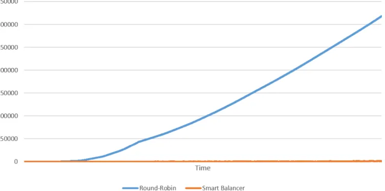
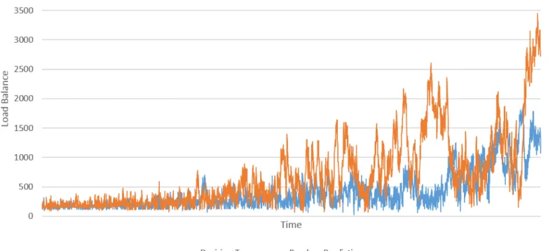
See Figure 2 for a comparison of the load balancers’ performance during the first experiment described in Section 3. This graph shows how both algorithms behave under consistent, heavy load over a period of about 10 seconds. The smart balancer outperforms the round-robin balancer, because the load balancing measure is consistently lower and increases slower.

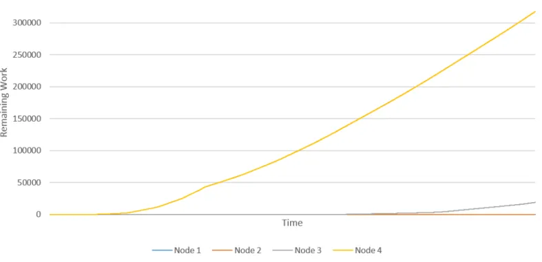
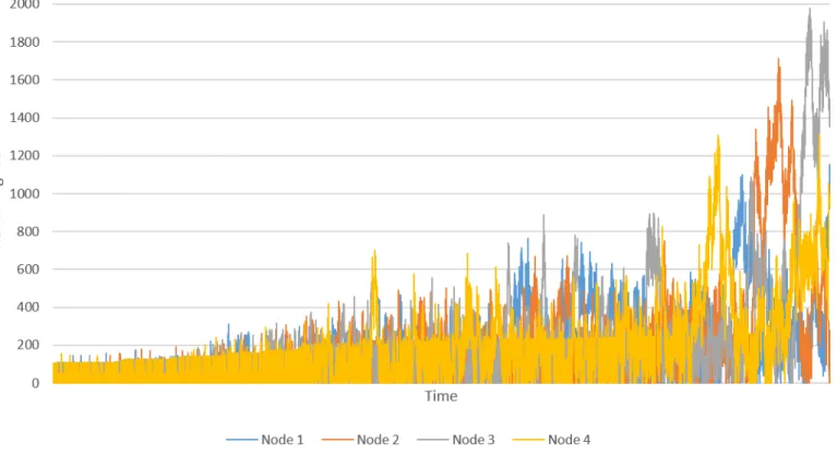
This Figure is based on the data from Figure 3 and 4. Note that the scales on these two figures are different; the smart load balancer keeps the load consistently more spread over the nodes than the round-robin approach. This is likely also the cause for the spikes that appear in the graph. ’Remaining work’ in these graphs is the amount of milliseconds (as measured in the real system) are left on each node.

Figure 2: Load balance as measured during experiment 1.

See Figure 5 for a comparison of the load balance during experiment 2. Although neither graph is smooth, the decision tree-based balancer outperforms the random-based balancer, because it’s measure is lower and it increases slower. It is also less spiky, which indicates more consistent load. Note that the measure increases for both balancers towards the end of the experiment, because the load on all nodes increases.

(9)

Figure 3: Remaining work on each node as measured during experiment 1, for the round-robin load balancer.

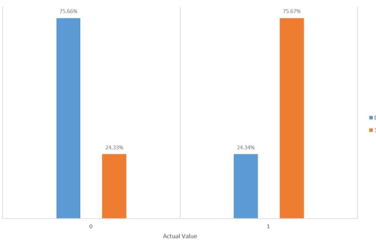
See Figure 6 for an overview of the performance of the predictor. Although the tree only predicts around 75% accurately, it has a big impact on the performance of the load balancer.

(10)

Figure 4: Remaining work on each node as measured during experiment 1, for the smart load balancer.

(11)

(12)

(13)

5 Conclusion

The results of both experiments (see Section 3) is positive: the results indicate that the smart load balancer performs better than round-robin and that the balancer using the decision tree performs better than the one using random guesses.

Since the data that was used to build the decision tree contains system-specific information, such as URLs, service names and whether a cookie was present, this approach will capture such domain-specific information without losing general applicability.

A potential problem with the system is that it can get out of sync with the real balance on nodes. This can occur, because it only ever predicts the load on each node, it doesn’t receive any actual data on the state of the system. As a result of this, it can occur that the predictor makes many poor predictions in a row, and the load becomes unbalanced. This situation will resolve itself when there is a period of low traffic, which is not uncommon in most systems.

5.1 Future work

Although the system performs quite well in comparison to round-robin, a compar-ison study to other algorithms could be performed. The results of this can likely improve its performance. In addition, different machine-learning algorithms can be tested, and the learning algorithm can be better tailored to the domain. Finally, the algorithm could be adapted to a situation where the number of nodes is dynamic.

In the sample data used in this paper, two clusters were present in the response data. This is not necessarily true for any data set. A study could be done of how response times behave in complex systems after measurements over long periods of time. This could provide data to choose a different learning algorithm that behaves better in the general case.

Although there are some points for improvement, the demonstrated algorithm does provide a significant improvement over the one that is currently in use in a real world application, and is flexible enough to be adaptable in a more general setting. It delivers on the goal of a load balancer, to decrease the average response time with the same resources.

(14)

References

Altman, Eitan, Urtzi Ayesta, and Balakrishna J Prabhu (2011). “Load balancing in processor sharing systems.” In:Telecommunication Systems47.1-2, pp. 35–

48.

Aruna, M, D Bhanu, and R Punithagowri (2013). “A Survey on Load Balancing Algorithms in Cloud Environment.” In:International Journal of Computer Applications82.16, pp. 39–43.

Begum, Suriya and CSR Prashanth (2013). “Investigational Study of 7 Effective Schemes of Load Balancing in Cloud Computing.” In:International Journal of Computer Science Issues (IJCSI)10.6.

Doroudi, Sherwin, Esa Hyytiä, and Mor Harchol-Balter (2014). “Value driven load balancing.” In:Performance Evaluation79.0. Special Issue: Performance

2014, pp. 306 –327. issn: 0166-5316. doi: http://dx.doi.org/10.1016/j.

peva.2014.07.019.url: http://www.sciencedirect.com/science/article/pii/

S0166531614000820.

Mukhopadhyay, Arpan, A. Karthik, and Ravi R. Mazumdar (2015). “Randomized Assignment of Jobs to Servers in Heterogeneous Clusters of Shared Servers for Low Delay.” In:CoRR abs/1502.05786._url: http://arxiv.org/abs/1502.