Autotuning Techniques for Performance-Portable Point Set Registration in 3D

Autotuning Techniques for Performance-Portable Point Set

Registration in 3D

Piotr Luszczek1_{, Jakub Kurzak}1_{, Ichitaro Yamazaki}1_{, David Keffer}2_, Vasileios Maroulas3_{, Jack Dongarra}1,4,5

c

The Authors 2018. This paper is published with open access at SuperFri.org

We present an autotuning approach applied to exhaustive performance engineering of the EM-ICP algorithm for the point set registration problem with a known reference. We were able to achieve progressively higher performance levels through a variety of code transformations and an automated procedure of generating a large number of implementation variants. Furthermore, we managed to exploit code patterns that are not common when only attempting manual optimization but which yielded in our tests better performance for the chosen registration algorithm. Finally, we also show how we maintained high levels of the performance rate in a portable fashion across a wide range of hardware platforms including multicore, manycore coprocessors, and accelerators. Each of these hardware classes is much different from the others and, consequently, cannot reliably be mastered by a single developer in a short time required to deliver a close-to-optimal implementation. We assert in our concluding remarks that our methodology as well as the presented tools provide a valid automation system for software optimization tasks on modern HPC hardware.

Keywords: portable performance engineering, point set registration, autotuning with code generation, combinatorial optimization.

Introduction

Many aspects of computer vision commonly uses algorithms for registration of point sets in three-dimensions (3D). But in many areas of science, these methods can be used for analyzing 3D data arriving from experimental hardware instruments. In particular, this is necessary in order to produce unambiguous descriptions of atomic-scale structures from large data sets originating in Atomic Probe Tomography (APT) [15, 19] and multimodal electron microscopy (EM) [14, 24]. In the study and design of High Entropy Alloys (HEAs), APT can generate data sets that include from 106 to 107 atoms in a single frame. Work is underway for electron microscopes to relay time-resolved frames, resulting in an explosion of data that truly puts the analysis of the output of these analytical techniques of registration squarely within the realm of “big data” analytics. The ultimate goal, when processing APT data sets, is to be able to resolve both atomic identity and atom position. The incoming instrument data is in the form of sets of atomic coordinates

(x, y, z) in three-dimensional (3D) space accompanied by identification of the atom type. Such

data is in many ways similar, in its basic form, to visualization tasks but the registration of the points will be followed by derivation of physics, chemistry, or material science profiles that inform the scientists of emergent properties of the analyzed samples. This serves as a motivation for fast and accurate implementations of the registration algorithms that are the subject of this paper. In order to arrive at novel properties such as resistance to high-temperature, corrosion, fracture and fatigue [8, 26], large amount of work has been performed to evaluate various techniques for characterizing local atomic environments [1]. To a significant extent, we follow here a similar approach and adopt tools from image reconstruction and pattern analysis in the

1_{Innovative Computing Laboratory, University of Tennessee, Knoxville TN, US}

2_{Department of Materials Science & Engineering, University of Tennessee, Knoxville TN, USA} 3_{Department of Mathematics, University of Tennessee, Knoxville TN, USA}

4_{Oak Ridge National Laboratory, Oak Ridge TN, USA}

generic field of machine vision in order to construct detailed atomic structures with highly-resolved locations from often defective data sets, especially those coming from APT experiments. Mathematically, of most importance is the minimization of the Frobenius norm: _{k · k}F; computed for a set of matrices representing the difference between a model reference configuration, m, denoting the true, average local structure, and the local configuration (data),di, around atom i, where for an APT experiment,iranges from 1 to k≈107:

min Ri,Pi

k X

i=1

km−PidiRik2_F, (1)

where each configuration has a unique permutation,Pi, and rotation,Ri, matrix (both real and orthogonal) in order to make it invariant to the arbitrary orientation and numbering generated by the experimental process.

A formulation of the problem that is based on Bayesian principles is under development and it explores Markov chain Monte Carlo scheme. A more classic approach is taken here to espouse benefits of autotuning whereby automation is applied to efficient evaluation of a large variety of implementation variants. In particular, we use Expectation-Maximization (EM) Iterative Closest Point (ICP), or EM-ICP for short. EM-ICP is a stochastic method for registration of surfaces. It improves issues found in other algorithms related to minimizing non-convex cost function. Other registration algorithms are given in Section 1.

In a simplified yet generic mathematical form, registration of point sets X=_{xi|xi ∈Rd} and Y =_{yi|yi ∈Rd} may be expressed as:

min

f∈T kf(X)−Yk, (2)

where the point sets come from a 3D space (rather then a space of arbitrary dimensiond):

X=_{x1, x2, . . . , x`}, Y ={y1, y2, . . . , ym} withxi, yj ∈R3 (3)

and the function f, drawn from the eligible set of transformations _T, is in our case a simple linear transform chosen to represent a combination of rotation, scaling, and translation:

f :X_7→R_×X+t_≡Y (4)

these restrictions result in a transformation that is called rigid registration and is the primary focus of this manuscript. However, a more general non-rigid registration is possible and it allows the transformation to be affine. For such a case, it is possible to include anisotropic scaling and skews. Furthermore, a generalization is possible which allows as input an unknown point set. This is close to the APT data sets which by their very nature cannot account for all atoms in the sample. Note also the noise resilience whereby the original formulation is often assumed to be robust to input measurement errors in the sense that it can handle a distribution of errors imposed on input data with either outliers or some points missing or both. Again, this caters directly towards APT-generated point clouds.

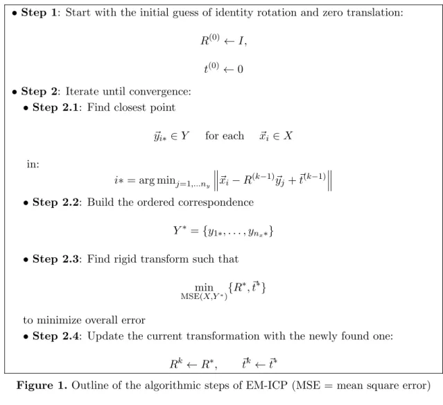
A much-simplified overview of the EM-ICP algorithm is depicted in Fig. 1. Starting with the initial guesses for the components of the transformation as an identity rotation and zero scaling matrix R(0) _{and zero translation matrix t}(0) _{which consequently get updated in an iterative}

•Step 1: Start with the initial guess of identity rotation and zero translation:

R(0) _←I,

t(0) _←0

•Step 2: Iterate until convergence:

• Step 2.1: Find closest point

~yi∗ ∈Y for each ~xi∈X

in:

i_∗= arg min_j=1,...ny~xi−R(k−1)~yj+~t(k−1)

• Step 2.2: Build the ordered correspondence

Y∗ =_{y1∗, . . . , ynx∗}

• Step 2.3: Find rigid transform such that

min

MSE(X,Y∗₎{R

∗_{, ~t}∗_}

to minimize overall error

• Step 2.4: Update the current transformation with the newly found one:

Rk_←R∗, ~tk _←~t∗

Figure 1. Outline of the algorithmic steps of EM-ICP (MSE = mean square error)

The rest of the article is organized as follows. Section 1 is devoted to a short survey of the related work. In Section 2, we present performance profiles of the implementations of the registration algorithm under consideration. Section 3 contains detailed performance results on various hardware platforms. Section 4 discusses in more detail some the important aspects of the results. The conclusion section summarizes the study and points to potential directions for further work.

1. Related Work

The algorithm called Iterative Closest Point (ICP) [2, 27] has two important properties: simple implementation structure and the low levels of computational cost. This characterization on both counts has resulted over time in increased popularity and both of these aspects have contributed to proliferation of numerous variants [7, 22] including the one we consider here in more detail called EM-ICP [10]. The Expectation Maximization (EM) algorithm for Gaussian Mixture Model (GMM) may be shown [3] to be equivalent to Robust Point Matching (RPM) algorithm [9] that alternates soft-assignment of correspondences and transformation. Multiple versions of RPM have been developed [4, 5, 21]. Finally, there is Coherent Point Drift (CPD) algorithm [20] which performs the so called non-rigid registration while using a suitable regularizer.

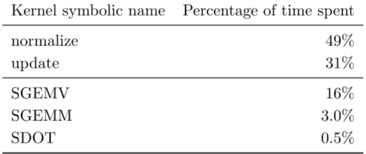
Table 1.Performance profile of EM-ICP implementation in CUDA running on NVIDIA Kepler accelerator

Kernel symbolic name Percentage of time spent

normalize 49%

update 31%

SGEMV 16%

SGEMM 3.0%

SDOT 0.5%

implementations. Parallel counterparts based on OpenMP or explicit multithreading for multicore processors are rare. Even more so are enhancements for hardware accelerators and we attempt to breach that gap. For example, some support for ICP is available, in the Point Cloud Library (PCL) [23] as part of a larger set of methods. Some of these codes may be used as the basis for our implementations but they require changes for efficiency. Additionally, we perform updates to make them adhere to the modern software stack [18]. More specifically, we needed to introduce the current version of CUDA which is better than what is available in the code with CUDA version 5 being the last supported release. Additionally, by adding utilization of the GPU hardware platforms, we expanded test results. Some implementations6 _{could potentially be adapted with}

cosmetic adjustments to allow them to use more recent versions of CUDA such as version 6.5 but this is not a guarantee of good performance. In summary, the implementations we generate are highly customized and target the most recent versions available and supported by NVIDIA: 7.5 and 8.0 with initial work towards compatibility with even newer releases of CUDA 9.0 and 10.0. Unfortunately, these latest versions of CUDA were not widely available to the public during the initial test runs.

2. Analysis of Bottlenecks based on Code Profiling

Our survey of existing codes for EM-ICP revealed that the freely available implementations7

focus on visualization tasks and image processing workflows that are often optional in case of scientific instruments. Our focus is to provide very high ingest rates of the data coming from the hardware sensors. Our goal is to automatically derive an implementation that is able to process them in time before the long-term storage system becomes overwhelmed. Based on a survey of available solutions, we concluded that their support for High Performance Computing (HPC) techniques is poor and we faced the choice of retrofitting the codes for multithreading, modern accelerator libraries, and performance profiling or write our own version from scratch. We chose the former and used this updated code as a reference point that we optimized on a variety of modern HPC platforms.

As the first step in the performance engineering, we acquired an application profile and identified the bottleneck portions of the code that may then be targeted with our autotuning methodology in order to maximize the potential speedup benefits. Table 1 shows a typical performance profile on one of the tested devices. It is representative of the time breakdown that

6_{One such implementation is ICPCUDA available athttps://github.com/mp3guy/ICPCUDA.}

7_{We did not consider commercial implementations for this study but only the codes that can be obtained under}

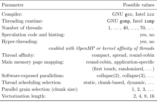
Table 2.Autotuning parameter space used for optimization of performance through OpenMP parallelization and directives

Parameter Possible values

Compiler: GNU gcc, Intel icc

Threading runtime: GNU gomp, Inteliomp Number of threads: 1, . . . , 40, . . . , 70, . . . Speculation code and hinting: yes, no

Hyper-threading: yes, no

enabled with OpenMP or kernel affinity of threads

Thread affinity: compact, spread, round-robin Main memory page mapping: round-robin, application-specific (first touch, randomized, . . . ) Software-exposed parallelism: collapse(2), collapse(3), . . . Thread scheduling selection: static, chunk-based, dynamic, . . . Parallel grain selection (chunk size): 1, 2, 3, . . .

Vectorization length: 2, 4, 8, 16

we observed on the other machines used in tests. Note that this represents less computationally-intensive variant of the ICP method than has been reported by approaches that used Singular Value Decomposition (SVD) at each iteration [6]. The codes for point set registration require 32-bit floating-point arithmetic for computation and hence most of the code uses single-precision float data types and the profile from the figure uses that precision and changes to this will be explicitly noted. Also, the experimental hardware such as APT generates data that can be accurately represented in 32-bit floating-point digits.

The common technique for efficient implementations is to off-load the compute-intensive parts of the code to highly tuned numerical libraries. In the case of results from Tab. 1, the calls to NVIDIA CUBLAS make optimal use of the compute units (SGEMM) and the available memory bandwidth (SGEMVandSDOT). Unfortunately, once these sections of the code achieve the state close to hardware-optimal performance, the other parts of the code become the main sources of slowdown. These two slowdown parts are namedupdateandnormalize. In terms of the operations from algorithm in Fig. 1, they represent updates and normalization of the correspondence and error metrics throughout the iterations. Focusing on these two portions exclusively targets nearly 90% of the execution time across our tested hardware.

Once we identified the code sections that are important for performance engineering, we pro-ceeded with defining the parameter space of available configurations that need to be explored for generating code that would execute efficiently. Table 2 shows a summary of that space for multicore hardware (GPU-specific considerations are presented below) with open source8 and commercially developed9 software stack. The search space for autotuning optimization is multidimensional and heterogeneous in the sense that it includes different categories of parameters, namely: binary

8_{Due to the fact that the GNU and LLVM compilers share the OpenMP runtime, we only considered GNUgomp}

but a LLVM-specific solution is under development.

9_{We only considered one commercial compiler but other choices are also possible, for example the PGI Group or}

compiler = ("gcc", "icc") runtime = ("gomp", "iomp") omp num threads = range(1, 75) speculation = (False, True) hyper threading = (False, True)

kmp affinity = ("disabled", "compact", "scatter")

gomp cpu affinity = ("1-75:1", "1-75:2", "1-75:3", "1-75:4") omp palces = ("none","threads","cores", "sockets")

omp proc bind = ("close", "master", "spread","none") memory affinity = ("round robin", "random", "first touch") collapse = (1, 2, 3)

schedule = ("default", "static", "chunk", "dynamic") schedule size = range(0, 64+1)

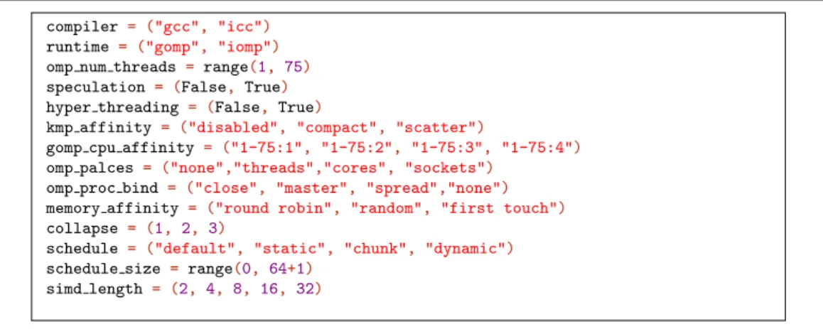
simd length = (2, 4, 8, 16, 32)

Figure 2. Definition of the autotuning space for multicore and manycore CPUs

values (for example use, hyperthreading or not use it), ordinal/categorical/enumeration values (for example, compiler-version pairs: gcc6.0, gcc7.0,icc2016, icc2017), integer values (for example, an integer range of loop blocking parameter values), and continuous variables (for example, cache reuse ratio). Theoretically, the entire search space may be represented by a Cartesian product of these variables which would result in combinatorial explosion in the size of the search space. In practice, the search space is much less regular due to a number of software and hardware constraints. Some examples include:

• The problem to be optimized might be solved for the GNU compiler but is an issue for the Intel compiler due to unknown internal issues.

• The output results might be changing depending on the version of the compiler: of-ten a newer version produces binaries whose results are an improvement but sometimes performance regressions may also occur.

• The interactions that are internal to the compiler, its OpenMP runtime implementation, OS version, and finally the processor firmware could further complicate the produce optimization results.

We have developed Domain Specific Language (DSL) to assist the autotuning processes. It is called LANAI (LANguage for Autotuning Infrastructure) [16]. It deals primarily with the definition of search space for optimal implementation. While further details certainly go beyond the current scope, for completeness, we feel compelled to include some information how the symbolic description of the parametric space from Tab. 2 translates into a LANAI description that we present in Fig. 2. Due to the way we presented the search space constraints in the table, the code from the figure may be considered self-explanatory. However, the full complexity of LANAI is beyond the scope of this manuscript and includes parsing of the autotuning specification (ranges, constraints, and their mutual dependence), multiple stages of optimization that reduce the autotuning time, and code generation that allows search space exploration to take place at the speed of a native code without the need to ever write such a code by hand.

2.1. Optimizations specific to NVIDIA GPUs and CUDA Software Stack

Table 3.Optimization space for a single kernel based on CUDA parallelization features

Parameter description Possible values

Read coalescing for input pointsX Yes / No Write coalescing for output points Y Yes / No Thread grid shapeGi×j i, j∈ {1, . . . ,1024}

Thread block shapeTR×C R, C∈ {1, . . . ,1024}

Amount of Shared Memory used {0,210,211, . . . ,216}

SM or SMX streaming unit utilization {1,2, . . . ,80}

(number of CUDA streams)

Active threads per thread {8,16,32}

Data affinity for grid-block: Gi×j×TR×C _→RX×Y _{row/column-wise, mixed} Floating-point precision 16-bit, 32-bit, 64-bit

Verification criteria Allowed values

GPU occupancy‡ 30%_÷95%

‡_{NVIDIA provides occupancy calculator for users. Good performance is not necessarily equivalent}

to good occupancy but there exist occupancy thresholds that are almost always well correlated with achieving sufficiently high levels of performance based on a relevant metric (bandwidth or compute intensity).

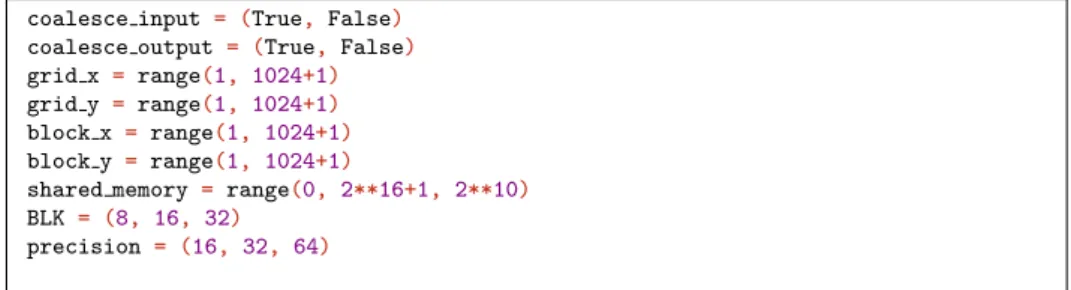
coalesce input = (True, False) coalesce output = (True, False) grid x = range(1, 1024+1) grid y = range(1, 1024+1) block x = range(1, 1024+1) block y = range(1, 1024+1)

shared memory = range(0, 2**16+1, 2**10) BLK = (8, 16, 32)

precision = (16, 32, 64)

Figure 3. Definition of the autotuning space for GPUs

to the main memory. The memory hierarchy of GPUs is shallower and often features smaller caches that are shared on a per-device basis. Despite these differences, the breakdown of execution time from Tab. 1 is generally applicable to both types of compute platforms. Furthermore, this similarity applies across multiple GPU devices and compiler tool chains which might feature, for example, different approaches to instruction predication and branch removal algorithms. Such details depend on availability of Special Function Units (SFUs) on the target device and the hardware’s predication window length. As a practical example, consider the difference between NVIDIA’s Kepler and Maxwell architectures: the former features a high end compute cards and has full support for 64-bit precision floating point arithmetic while the latter only targets gaming and rending markets with 32-fold slowdown of 64-bit instructions.

To maximize the bandwidth achieved by our implementation, we aim at efficient use of global and shared memory banks as well as enforcement of coalesced reads through stride-1 accesses. This is done explicitly since the GPU compilers often do not automatically handle Instruction-Level Parallelism (ILP). Also by design, CUDA shifts the burden of exposing the Thread-Level Parallelism (TLP) to the user as the threads must be explicitly created and managed by the user code inside kernel functions. These considerations result in a modified search space for the GPU-optimized autotuning that is shown in Tab. 3.

As was the case for CPUs, Tab. 3 may be translated almost directly into LANAI specification shown in Fig. 3. There is a number of important issues worth noting. Because the grid and block dimensions are specified independently, for some combinations of dimensions the thread counts will exceed what’s allowed on the GPU hardware. This may be counteracted with the LANAI’s so called constraint or it may be left to the CUDA compiler and runtime: one of them will indicate insufficient resources for launching a kernel. Clearly, the former solution is preferred because it limits the overall size of the search space and consequently speeds up the autotuning process. On the other hand, GPU occupancy is much more vague criteria to meet as it needs to be calculated in a more complicated way and, additionally, it never had a very well-defined relation with achieved performance across a wide range of codes [25]. Nevertheless, it can still be used in the optimization process to either prune the search space or terminate the performance tests early when they fail to meet a predetermined occupancy requirement.

2.2. Using Limited Precision Arithmetic

2.2.1. Hardware Landscape for 16-bit Floating-Point

A new type of hardware extension for 16-bit floating-point precision arithmetic (FP16) has become much more main stream in the past few years. Initial experiments in deep network training with limited floating-point accuracy [11, 12] validated this for machine learning methods. Since then, a numerous hardware vendors and supercomputing sites have been involved with the trend that links computational Artificial Intelligence and HPC. Consider the announced AMD GPUs MI5, MI8, MI25 whose model number corresponds to the peak performance of the card in FP16: 5 Tflop/s, 8 Tflop/s, and 25 Tflop/s, respectively. Softbank’s subsidiary ARM, announced publicly an extension to its NEON Vector Floating Point (VFP) to include FP16 in the V8.2-A architecture specification. NVIDIA GPUs that feature FP16 are widely available starting with Tegra TX1 and Pascal P100 cards. NVIDIA’s Volta-based V100 and DG100 and the Xavier car platform feature further extensions of the FP16 support. TSUBAME 3 is one of the first supercomputers to prominently feature FP16 but other sites with NVIDIA Pascal hardware can fully utilize this new functionality. This is in line with our experiments in using FP16 in HPC benchmarking [17]. The ISO C++ standard is slated to addshort float primitive data type that will likely be also added the C standard document following the IEEE 754-2018 specification and current support of Float16primitive data type.

2.2.2. FP16 Considerations for Point Set Registration

Table 4.FP16 and Its Hardware Support IEEE 754 (2008)

Precision Width Exponent Mantissa Epsilon Max

Quadruple 128 15 112 _O(10−34₎

O(104932₎

Extended 80 15 64 _O(10−19₎

O(10308₎

Double 64 11 52 _O(10−16₎

O(10308₎

Single 32 8 23 O(10−7_{) O(10}38₎

Half† 16 5 10 O(10−3_{) 65504}

† _{defined only for storage}

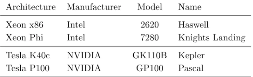
Table 5.Summary of hardware platforms used in the performance tests

Architecture Manufacturer Model Name

Xeon x86 Intel 2620 Haswell

Xeon Phi Intel 7280 Knights Landing

Tesla K40c NVIDIA GK110B Kepler

Tesla P100 NVIDIA GP100 Pascal

compute in FP32 arithmetic but consume FP16 operands. This is similar to the common practice of the way the Fused-Multiply-Add (FMA) instruction is implemented with higher precision for the intermediate results.

From the perspective of point set registration, FP16 has a potential benefit of increased bandwidth and vastly improved compute intensity. The former affords a 2-fold increase on the NVIDIA Pascal cards. The primary consideration is the limited range of the FP16 values as shown in Tab. 4. At the basic algorithmic level, the use of limited precision in most calculations may serve as a opportunistic regularization scheme which, among other things, could prevent overfitting the model to noisy input data as is the case in some scenarios.

3. Performance Results

3.1. Description of the Tested Hardware Platforms

Our autotuning experiments were performed on a number of hardware platforms including multicore, manycore, and GPU accelerators. A quick summary of these machines is given in Tab. 5. Out of the computers shown in the table, Intel Phi KNL could potentially be the newest and might be the least familiar to the reader. As an alternative to the superscalar x86, it represents a new architecture10from Intel that is solely based on low-power Atom Silvermont cores with the maximum of 72 cores in a chip connected with a mesh interconnect and divided logically into 4 so called quadrants with NUMA-like characteristics as far as data affinity is concerned. However, further details on cache and memory hierarchy with on-chip specification is out of scope of this article. Initially planned for two major hardware versions as either self-boot (self-hosted) or leveraged-boot (accelerator) units. Currently, only self-boot units are commercially available.

10_{Note that for the most part Xeon and Xeon Phi processors are binary compatible with the exception of the}

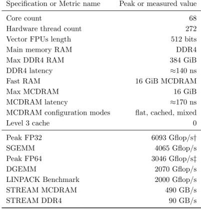
Table 6.Detail characteristics of the Intel Xeon Phi Knights Landing platform a manycore CPU used in the tests with the performance numbers coming from hardware specification or the vendor testing

Specification or Metric name Peak or measured value

Core count 68

Hardware thread count 272

Vector FPUs length 512 bits

Main memory RAM DDR4

Max DDR4 RAM 384 GiB

DDR4 latency ≈140 ns

Fast RAM 16 GiB MCDRAM

Max MCDRAM 16 GiB

MCDRAM latency ≈170 ns

MCDRAM configuration modes flat, cached, mixed

Level 3 cache 0

Peak FP32 6093 Gflop/s†

SGEMM 4065 Gflop/s

Peak FP64 3046 Gflop/s_‡

DGEMM 2070 Gflop/s

LINPACK Benchmark 2000 Gflop/s

STREAM MCDRAM 490 GB/s

STREAM DDR4 90 GB/s

†68_×1.4 GHz_×2 VPUs_×FMA_×16 AVX lanes ‡68_×1.4 GHz_×2 VPUs_×FMA_×8 AVX lanes

The relevant details on the Intel Xeon Knights Landing (KNL) machine are given in Tab. 6 as they are available from public sources.

3.2. Application-Specific Performance Metric for Cross-Platform Comparisons: Derivation of the Performance Rate

maximize the number of floating-point instructions that often come free as long as they are executed on data residing in Level 1 cache. Unfortunately, such operations contribute very little to the applications’ ultimate goal that need faster execution for large memory footprints that do not fit in any cache level all at once. Instead, we derive an application-relevant metric based on the asymptotic performance theory [13].

For registration problems in particular, the performance metric we choose as relevant is the number of points in the cloud registered per second. Using this provides with a rate and we can quickly compare either images, scenes or surfaces that contain different number of points. Simultaneously, we are still able to map the rating back to time-to-solution when we know the exact point-count. We use Giga-points-per-second (Gpts) as the unit for the execution rate that is defined as:

r = t

nXnY

10−9 Gpts,

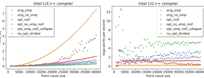
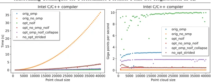
wherenX andnY represent the number of the input and output points, respectively. The scaling factor of 10−9 is a standard SI prefix that allows all of the rates measured in this article to fall within the range of small numbers that are less than 50 that are familiar and human readable. The charts in the right of Fig. 4, Fig. 5, and Fig. 6 show this new metric applied to the timing charts shown in the left of the respective figures. As an added advantage, we are able to see subtleties of the optimal configurations. It turns out that in Fig. 5 the asymptotic performance rate is nearly 6 Gpts but the cache effects may be observe all the way until point clouds of size 5000 points when the working set fits in highest levels of the cache hierarchy and the performance rate is higher due to the much higher cache bandwidth and lower access latency of fetch image data.

Finally, rather than presenting a speedup, we only show all the performance results of all tested configurations without specifying the reference and most optimal ones. This enables the reader to see the range of results that may be observed in practice. Due to the automated way of obtaining the results, we can guarantee minimal human intervention while obtaining a fast implementation.

3.3. Timing and Performance Rate Results for GNU and Intel Compilers on the x86 Machine

0 5000 10000 15000 20000 25000 30000 35000 40000 Point cloud size

0 5 10 15 20 25 Time [s]

GNU C/C++ compiler version 5.3

orig_omp orig_no_omp opt_noif opt_no_omp_noif opt_omp_noif_collapse no_opt_strided

0 5000 10000 15000 20000 25000 30000 35000 40000 Point cloud size

0.0 0.2 0.4 0.6 0.8 1.0 1.2 1.4

Giga points per second

GNU C/C++ compiler version 5.3

orig_omp orig_no_omp opt_noif opt_no_omp_noif opt_omp_noif_collapse no_opt_strided

Figure 4. Point set registration timing and performance results on the x86 Haswell machine with the GNU compiler for various OpenMP configurations and the colors on left and right charts represent the same configurations

0 5000 10000 15000 20000 25000 30000 35000 40000 Point cloud size

0 1 2 3 4 5 6 7 Time [s]

Intel C/C++ compiler

orig_omp orig_no_omp opt_noif opt_no_omp_noif opt_omp_noif_collapse no_opt_strided

0 5000 10000 15000 20000 25000 30000 35000 40000 Point cloud size

0 2 4 6 8 10 12

Giga points per second

Intel C/C++ compiler

orig_omp orig_no_omp opt_noif opt_no_omp_noif opt_omp_noif_collapse no_opt_strided

Figure 5. Point set registration timing and performance results on the x86 Haswell machine with the Intel compiler for various OpenMP configurations and the colors on left and right charts represent the same configurations

the GNU compiler, we did not conduct any further experiments to understand whether this may be related to either the generated instruction mix or more efficient OpenMP runtime. We leave this and other questions of such sort for future work based on similar hardware and software stacks. Also, we will no longer present GNU compiler results due to low observed performance. A detailed analysis of the instruction stream generated by GNU and Intel compilers is beyond the scope of this manuscript and we only attempted to use for both compilers similar flags including highest possible optimization level and relaxed floating point model to make aggressive code generation possible.

3.4. Timing and Performance Rate Results on Many-core KNL System and GPU Device Cards

Figure 6 presents the timing and performance rate results on the Intel Xeon Phi KNL machine. Two clear differences may be observed when comparing against x86 results:

0 5000 10000 15000 20000 25000 30000 35000 40000 Point cloud size

0 5 10 15 20 25 30 35

Time [s]

Intel C/C++ compiler

orig_omp orig_no_omp opt_noif opt_no_omp_noif opt_omp_noif_collapse no_opt_strided

0 5000 10000 15000 20000 25000 30000 35000 40000 Point cloud size

0 2 4 6 8 10

Giga points per second

Intel C/C++ compiler

orig_omp orig_no_omp opt_noif opt_no_omp_noif opt_omp_noif_collapse no_opt_strided

Figure 6.Point set registration timing and performance results on the Xeon Phi Knights Landing machine with the Intel compiler for various OpenMP configurations and the colors on left and right charts represent the same configurations

0

5000 10000 15000 20000 25000 30000 35000 40000

Point cloud size

0

10

20

30

40

Giga points per second

All runs combined

Figure 7. Point set registration performance rate results on the NVIDIA Pascal P100 card with the NVIDIA nvcccompiler for all loop blocking configurations and these results are shown for reference only to give the reader an idea of how many runs were performed, how they cluster, and range across point cloud sizes

• the variability of timing measurements is not present on KNL and the graphs are much more smooth especially for the data sizes when the working set exceeds the cache size and the data has to be streamed from the main memory. This may be attributed to the short speculative execution window in the KNL’s execution unit design.

First, Fig. 7 shows all data points collected from running on the P100 card in FP32. Clearly presented in that manner, it is hard to discern specific properties that contributed to the achieved performance levels. We do so in the analysis that follows by taking into account the various hardware features that are specific to GPUs and how they affect the performance of various point set registration implementations.

0 5000 10000 15000 20000 25000 30000 35000 40000

Point cloud size

0

1

2

3

4

5

6

7

8

Giga points per second

BLK=2.0

BLK=4.0

BLK=6.0

BLK=8.0

BLK=10.0

BLK=12.0

BLK=14.0

BLK=16.0

BLK=18.0

BLK=20.0

BLK=22.0

BLK=24.0

BLK=26.0

BLK=28.0

BLK=30.0

BLK=32.0

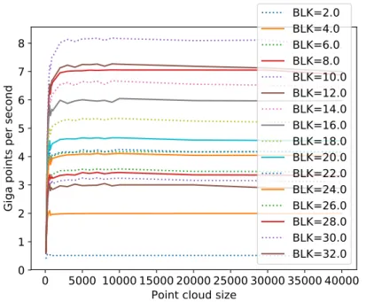
Figure 8.Point set registration performance rate results on the NVIDIA Kepler K40c card with the NVIDIA nvcc compiler for various loop blocking configurations with non-coalesced reads

0 5000 10000 15000 20000 25000 30000 35000 40000

Point cloud size

0

2

4

6

8

10

12

14

Giga points per second

BLK=2.0

BLK=4.0

BLK=6.0

BLK=8.0

BLK=10.0

BLK=12.0

BLK=14.0

BLK=16.0

BLK=18.0

BLK=20.0

BLK=22.0

BLK=24.0

BLK=26.0

BLK=28.0

BLK=30.0

BLK=32.0

Figure 9.Point set registration performance rate results on the NVIDIA Kepler K40c card with the NVIDIA nvcc compiler for various loop blocking configurations with coalesced reads

memory. This clearly goes against the common optimization guidance that is taught to GPU novice users. To show the effect of the problem and how it helps to fix it, Fig. 9 shows the configuration when the coalescent reads were used. The performance increase is nearly 2-fold which confirms the importance of this optimization for the registration code and for our tested implementations.

0 5000 10000 15000 20000 25000 30000 35000 40000

Point cloud size

0

2

4

6

8

10

12

14

16

Giga points per second

BLK=2.0

BLK=4.0

BLK=6.0

BLK=8.0

BLK=10.0

BLK=12.0

BLK=14.0

BLK=16.0

BLK=18.0

BLK=20.0

BLK=22.0

BLK=24.0

BLK=26.0

BLK=28.0

BLK=30.0

BLK=32.0

Figure 10.Point set registration performance rate results on the NVIDIA Kepler K40c card with the NVIDIA nvcc compiler for various loop blocking configurations without the use of shared

0

5000 10000 15000 20000 25000 30000 35000 40000

Point cloud size

0

10

20

30

40

50

Giga points per second

Best and Worst Performance Results

Figure 11. Point set registration performance rate results on the NVIDIA Pascal P100 card with the NVIDIAnvcc compiler for the best and worst autotuning configurations using FP16 arithmetic

it is possible to gain a percentage point or more in terms of performance if the shared memory is not used and the main memory is accessed directly.

3.5. Limited Precision Implementation

0

5000 10000 15000 20000 25000 30000 35000 40000

Point cloud size

0

10

20

30

40

50

Giga points per second

Best and Worst Performance Results for FP16 and FP32

FP16 fastest

FP32 fastest

FP32 slowest

FP16 slowest

Figure 12.Point set registration performance rate results on the NVIDIA Pascal P100 card with the NVIDIA nvcc compiler for the best and worst autotuning configurations using either FP16 or FP32 arithmetic

#pragma omp parallel for

for(i← 0;i < nX;i←i+1)

for(j← 0;j < nY;j←j+1)

. . .

#pragmaomp parallel for collapse(2)

for(i_← 0;i < nX;i←i+1)

for(j_← 0;j < nY;j←j+1)

. . .

Figure 13.Optimal Configuration for GNU Compiler on x86

FP16 instructions is twice as small and, consequently, it would be obvious to expect about a two-fold increase in performance for both compute-bound and bandwidth-bound codes. Both of these are present in the registration methods tested here.

// FP16-FP32 conversions contribute additional // overheads and hit against hardware limit cvt.f32.f16 f, r // convert from FP16 sqrt.approx.f32 f, f // compute in FP32 cvt.rn.f16.f32 r, f // convert to FP16

Figure 14.A Glance at PTX (NVIDIA’s Pseudo-Assembly)

4. Discussion on GNU and FP16 Results

Figure 4 singled out the GNUgcccompiler’s issues with generating optimized instruction mix for the registration code. Despite our efforts to enable optimized parallelization levels we saw the lack of efficiency in the use of multi-threading as it exhibited low core utilization rates which resulted in inferior execution speed. This potentially may be remedied by merging deep loop nests into a combined index set. That set is then divided (in some fashion) among the available OpenMP threads. This is done manually by inserting specifically crafted pragma directives. OpenMP standard specifiescollapse clause to have this loop-nest merging performed by the GNU compiler. Such an optimization may be applied as shown in Fig. 13. Our autotuning framework easily allows the user to introduce the clause conditionally in the generated code variants and then tests the resulting binaries with a number of loop-collapsing parameters. In the end, this allows the autotuning process to find out the optimal setting for the tested hardware platform and the software stack combination.

Also somewhat surprising result was uncovered during the autotuning process and may be observed in Fig. 12. What is shown is comparatively small difference between the performance obtained from the implementation variants that use either FP16 and FP32 floating-point arith-metic. As our analysis indicates, this may be fully attributed to the overhead of conversion instructions. We confirmed this information by analyzing the PTX assembly-level code produced by the NVIDIA nvcc compiler and PTX code generator. The PTX code in question is shown in Fig. 14 in a simplified style to focus on relevant code and with majority the extra details removed. Mixing FP16 and FP32 data on the same GPU engages the hardware conversion units on the NVIDIA Pascal chips and those are limited in number. Much fewer of these units are available when compared, for example, with floating point units in either FP16 and FP32 floating-point precisions. These conversions slow down the overall execution within a single GPU thread warp and contributes to the overall slowdown of the code. Clearly, any performance gains are squandered and we loose what might have been obtained from using FP16 precision if only enough hardware units were available. We observed this phenomenon while we performed autotuning procedure and otherwise it might have not been exposed if it was obstructed by other bottlenecks. It might have also been missed in an non-optimized or manually optimized code. This kind of effects occur mostly in automatically generated code and are otherwise hidden due to a limited exposure of the compiler to the large variety implementation variants that are possible through autotuning.

Concluding Remarks and Future Work

used it for 3D point clouds. In our tests, we applied a variety of automated transformations which resulted in an improved performance. We also used an automated process of generating a set of implementation variants. First, this allowed us to largely exceed the performance achieved by the reference code that was only optimized manually. Second, we searched the large parameter space of potential performance-oriented implementations to arrive at stable and portable performance levels. Those made the resulting EM-ICP codes available not on one but across a large range of hardware platforms and software stacks. In particular, our methodology and autotuning framework generated implementations for multicore, many-core, and accelerator-equipped machines.

We plan on extending this work to a wider range of algorithm that are available for the variants of the registration problem. Creating efficient codes for these methods is a natural future direction for us. We also intend to pursue more experimental approaches. However, due to a large number of algorithms and algorithmic variants for the point set registration problem, we intend to guide our selection of the promising method by the need of the relevant scientific fields. There are many such fields in need of point set registration implementations for analysis of large data sets such as APT experiments. These computational science fields benefit the most from our efforts in the performance engineering domain that we presented above. This is because we manage to achieve high execution rates which clearly contribute to ability to process large volumes of data coming from the experimental instrumentation tools such as Atomic Probe Tomography microscopes in material science and HEA material design.

Acknowledgements

This research was supported by United States National Science Foundation through grant 1642441.

This paper is distributed under the terms of the Creative Commons Attribution-Non Com-mercial 3.0 License which permits non-comCom-mercial use, reproduction and distribution of the work without further permission provided the original work is properly cited.

References

1. Bartok, A., Kondor, R., Csanyi, G.: On representing chemical environments. Physical Review B 87(18) (2013), DOI: 10.1103/PhysRevB.87.184115

2. Besl, P.J., McKay, N.D.: A method for registration of 3-D shapes. IEEE PAMI 14(2), 239–256 (1992), DOI: 10.1109/34.121791

3. Chui, H., Rangarajan, A.: A feature registration framework using mixture models. In: IEEE Workshop on MMBIA. pp. 190–197 (2000), DOI: 10.1109/MMBIA.2000.852377

4. Chui, H., Rangarajan, A.: A new algorithm for non-rigid point matching. In: CVPR. vol. 2, pp. 44–51. IEEE Press (2000), DOI: 10.1016/S1077-3142(03)00009-2

5. Chui, H., Rangarajan, A.: A new point matching algorithm for non-rigid registration. CVIU 89(2–3), 114–141 (2003), DOI: 10.1016/S1077-3142(03)00009-2

7. Fitzgibbon, A.W.: Robust registration of 2D and 3D point sets. Image and Vision Computing 21, 1145–1153 (2003), DOI: 10.1016/j.imavis.2003.09.004

8. Gao, M.C., Yeh, J.W., Liaw, P.K., Zhang, Y.: High-entropy alloys: fundamentals and applications. Springer International Publishing Switzerland (2016), DOI: 10.1007/978-3-319-27013-5

9. Gold, S., Lu, C.P., Rangarajan, A., Pappu, S., Mjolsness, E.: New algorithms for 2D and 3D point matching: Pose estimation and corresp. In: NIPS. vol. 7, pp. 957–964. The MIT Press (1995), DOI: 10.1016/S0031-3203(98)80010-1

10. Granger, S., Pennec, X.: Multi-scale EM-ICP: A fast and robust approach for surface registration. In: et al., A.H. (ed.) ECCV 2002. pp. 418–432. LNCS 2353, (c) Springer-Verlag Berlin Heidelberg (2002), DOI: 10.1007/3-540-47979-1 28

11. Gupta, S., Agrawal, A., Gopalakrishnan, K., Narayanan, P.: Deep learning with limited numerical precision. CoRR abs/1502.02551 (2015), http://arxiv.org/abs/1502.02551, accessed: 2018-08-01

12. Gupta, S., Agrawal, A., Gopalakrishnan, K., Narayanan, P.: Deep learning with limited numerical precision. In: Bach, F., Blei, D. (eds.) Proceedings of the 32nd International Conference on Machine Learning. Proceedings of Machine Learning Research, vol. 37, pp. 1737– 1746. PMLR, Lille, France (2015), http://proceedings.mlr.press/v37/gupta15.html, accessed: 2018-08-01

13. Hockney, R.W., Curington, I.J.: f1

2: A parameter to characterize memory and communication

bottlenecks. Parallel Computing 10(3), 277–286 (1989), DOI: 10.1016/0167-8191(89)90100-2

14. Kim, Y.M., Morozovska, A., Eliseev, E., Oxley, M., Mishra, R., Selbach, S., Grande, T., Pantelides, S., Kalinin, S., Borisevich, A.: Direct observation of ferroelectric field effect and vacancy-controlled screening at the BiFeO3/LaxSr1−xMnO3 interface. Nature Materials

13(11), 1019–1025 (2014), DOI: 10.1038/nmat4058

15. Larson, D., Prosa, T., Ulfig, R., Geiser, B., Kelly, T.: Local Electrode Atom Probe Tomogra-phy: A User’s Guide. Springer-Verlag New York (2013), DOI: 10.1007/978-1-4614-8721-0

16. Luszczek, P., Gates, M., Kurzak, J., Danalis, A., Dongarra, J.: Search space generation and pruning system for autotuners. In: Proceedings of IPDPSW. pp. 1545–1554. The Eleventh International Workshop on Automatic Performance Tuning (iWAPT) 2016, IEEE, Chicago, IL, USA (2016), DOI: 10.1109/IPDPSW.2016.197

17. Luszczek, P., Kurzak, J., Yamazaki, I., Dongarra, J.: Towards numerical benchmark for half-precision floating point arithmetic. In: 2017 IEEE High Performance Extreme Computing Conference (2017), DOI: 10.1109/HPEC.2017.8091031

19. Miller, M.K., Forbes, R.G.: Atom-Probe Tomography: The Local Electrode Atom Probe. Springer US (2014), DOI: 10.1007/978-1-4899-7430-3

20. Myronenko, A., Song, X., Carreira-Perpi˜n´an, M.A.: Non-rigid point set registration: Coherent Point Drift. In: Sch¨olkopf, B., Platt, J.C., Hoffman, T. (eds.) Advances in Neural Information Processing Systems 19. pp. 1009–1016. MIT Press (2007)

21. Rangarajan, A., Chui, H., Mjolsness, E., Davachi, L., Goldman-Rakic, P.S., Duncan, J.S.: A robust point matching algorithm for autoradiograph alignment. Medical Image Analysis 1(4), 379–398 (1997), DOI: 10.1016/S1361-8415(97)85008-6

22. Rusinkiewicz, S., Levoy, M.: Efficient variants of the ICP algorithm. In: Interna-tional Conference on 3D Digital Imaging and Modeling (3DIM). pp. 145–152 (2001), DOI: 10.1109/IM.2001.924423

23. Rusu, R.B., Cousins, S.: 3D is here: Point Cloud Library (PCL). In: IEEE Inter-national Conference on Robotics and Automation (ICRA). Shanghai, China (2011), DOI: 10.1109/ICRA.2011.5980567

24. Sohlberg, K., Rashkeev, S., Borisevich, A., Pennycook, S., Pantelides, S.: Origin of anomalous Pt-Pt distances in the Pt/Alumina catalytic system. ChemPhysChem 5(12), 1893–1897 (2004), DOI: 10.1002/cphc.200400212

25. Volkov, V., Demmel, J.W.: Benchmarking GPUs to Tune Dense Linear Algebra. In: Pro-ceedings of the 2008 ACM/IEEE Conference on Supercomputing. pp. 31:1–31:11. SC ’08, IEEE Press, Piscataway, NJ, USA (2008),http://dl.acm.org/citation.cfm?id=1413370. 1413402, accessed: 2018-08-01, DOI: 10.1145/1413370.1413402

26. Zhang, Y., Zuo, T.T., Tang, Z., Gao, M.C., Dahmen, K.A., Liaw, P.K., Lu, Z.P.: Microstruc-tures and properties of high-entropy alloys. Progress in Materials Science 61, 1–93 (2014), DOI: 10.1016/j.pmatsci.2013.10.001