CLASSIFICATION OF REMOTELY SENSED IMAGE USING RELEVANCE VECTOR MACHINE

(1)

88 CLASSIFICATION OF REMOTELY SENSED IMAGE USING RELEVANCE

VECTOR MACHINE

1

A.Kalarani, 2G.viji, 2S.Ramprakash

1

Assistant Professor, P.S.R.Rengasamy college of engg for women, Sivakasi.

2

Assistant Professor, P.S.R.Rengasamy college of engg for women, Sivakasi.

2

Lecturer, M.Kumarasamy College of Engg, Karur.

Abstract— This paper introduces a remotely sensed image classification method based on relevance vector machines (RVMs). The features of the remotely sensed image are extracted and the classification is done[4] with the help of those features. It is shown that approximately the good classification accuracy is obtained using RVM-based classification, with a significantly smaller relevance vector rate and, therefore, much faster testing time. This feature makes the RVM-based classification approach more suitable for applications that require low complexity and, possibly, real-time classification.

Index Terms—Classification, remotely sensed image

,Bayesian learning, relevance vector machines (RVMs).

I. INTRODUCTION

In the recent years, relevance vector machines (RVMs) have been successfully used in many application domains. In particular, the RVM constitutes a Bayesian approximation for solving generalized linear classification and regression models[1]. This method not only provides accurate predictions but also force sparsity (simplicity) of the method, and can produce confidence intervals for the predictions. Good trade-offs between accuracy and sparseness of the solution has been observed in many application domains. In the field of remote sensing, the use of RVM has been recently introduced for the prediction of biophysical parameters. Being a kernel-based method, the key point for obtaining good RVM classifiers is the definition of a suitable kernel function that can properly represent relations (similarities) among samples (pixels).

The advantages of the RVM are probabilistic predictions, automatic estimations of parameters, and the possibility of choosing arbitrary kernel functions. Most importantly, RVM classification results[9] in fewer

relevance vectors (RVs), classification can be carried out much faster with the RVM . For example, the RVM has been used for the detection of micro calcification clusters in digitalmammograms, and it has been shown that the RVM classifier is much more suitable for real-time processing and reduces the computational complexity while maintaining similar detection accuracy. It is proposed in this letter to utilize the RVM for

classification of remotely sensed images. This feature makes the RVM based classification approach more suitable for applications that require low complexity and possibly, real time classification.

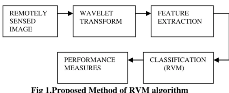
II. PROPOSEDMETHODOLOGY

Fig 1.Proposed Method of RVM algorithm

The proposed methodology classifies the remote sensed image based on RVM algorithm. In the first stage the remote sensed image is transformed using DWT .The approximated image is then chosen. The features of the approximated image were extracted .The extracted features were classified into

i)statistical features ii)textural features

The statistical features include i) mean ii) variance and iii) standard deviation. The textural features include i) energy ii) entropy iii) contrast and iv) homogeneity.The extracted features were taken as training and testing samples. The training and testing samples were classified using RVM algorithm and the performance were measured[12].

III.RVMCLASSIFICATION

Supervised learning techniques make use of a training set that consists of a set of sample input vectors

 

N n n

x

_₁ together with the corresponding targets

 

t

_n _nN_₁. The targets are basically real values in regression tasks or class labels in classification problems. It is typically desired to learn a model of the dependency of the targets on the inputs from the training set, so that accurate predictions of t can be made

REMOTELY SENSED IMAGE

WAVELET TRANSFORM

FEATURE EXTRACTION

CLASSIFICATION (RVM) PERFORMANCE

(2)

89

for previously unseen values of x[8]. Commonly, these predications can be based on some function y(x) defined over the input space in the form of

y



x

w



w

 

x

w

T

 

x

M

i











1

;

(1)

as a linearly weighted sum of M (generally nonlinear and

fixed) basis functions

 

   

 

T M

x



(



1

,



2

,...,



)



.

Although this model is linear in the parameters (or

weights),

w





w

₁_,

w

₂_,

...,

w

_M



T it can still be highly flexible as the size of the basis set M can be effectively large. Learning is basically the process of inferring the function or, equivalently, the parameters of the function y(x). In this context, it is desired to estimate reasonable values for the

parameters (or weights),

w





w

₁_,

w

₂_,

...,

w

_M



T. Given a set of N corresponding training pairs



x

_n

,

t

_n



N_n_₁, the objective is

to find values for the weights

w





w

₁_,

w

₂_,

...,

w

_M



T , such that y(x) generalizes well enough to new data, yet only a few elements of w are nonzero[5]. Having only a few nonzero weights facilitates a sparse representation with the advantage of providing fast implementation.

The RVM introduces a prior over the model weights governed by a set of hyper parameters , in a probabilistic framework. One hyper parameter is associated with each weight, and the most probable values are iteratively estimated from the training data[1]. The most compelling feature of the RVM is that it typically utilizes significantly fewer kernel functions , while providing a good performance. For two-class two-classification, any target can be two-classified into two classes such that

t

_n



 

0 ,

1

. A Bernoulli distribution can be adopted for p(t|x) in the probabilistic framework because only two values (0 and 1) are possible. The logistic sigmoid link function σ(y) = 1/(1 + e−y) is applied to y(x) to link random and systematic components, and generalize the linear model.

Following the definition of the Bernoulli distribution , the likelihood is written as

 





n









tn

n N

n

t

n

w

y

x

w

x

y

w

t

p

 







1

)

;

(

1 )

;

(

/



(2)

for the targets tn Є {0, 1}.The likelihood is complemented by a prior over the parameters(weights) in the form of





_       



 2 exp / 2 2 1 i i N i w w

p



i



 

(3)

where









1

,



2

,....,



N



T shows the hyper parameters introduced to control the strength of the prior over its associated weight[3]. Hence, the prior is Gaussian, but conditioned on



.For a certain



value, the posterior weight distribution conditioned on the data can be obtained using Bayes‘ rule, i.e.,





  



 



/

,

/

t

p

w

p

w

t

p

t

w

p



(4)

where p(t/w) is the likelihood, p(w/α) is the prior, and p(t)is referred to as evidence. The weights cannot be analytically obtained, and therefore, a Laplacian approximation procedure is used.1) Since p(w/t,α) is linearly proportional to p(t/w) × p(w|α), it is possible to aim to find the maximum of



 









 





t

y

t

y



w

Aw

w

p

w

t

p

T N n n n n n

2

1

1 log

/

log

1













(5)

for the most probable weights WMP, with yn= σ{y(xn;w)} and A = diag(α0, α1, . . . , αN) being composed of the current values of α. This is a penalized logistic log-likelihood function and requires iterative maximization. The iteratively reweighed least-squares algorithm] can be used to find WMP[6]. The logistic log-likelihood function can be differentiated twice to obtain the Hessian in the form of



w

t



w



B

A



p

w



_MP





T





log

/

,



|



(6)

where B= diag(β1, β2, . . . , βN) is a diagonal matrix with βn = σ{y(xn;w)}[1 − σ{y(xn;wMP)}], and Φ is the ‗design‘ matrix with Φnm= K(xn, xm−1) and Φn1 = 1. This result is then negated and inverted to give the covariance Σ, as shown as follows[12], for a Gaussian approximation to the posterior over weights centered at WMP.

Σ = (ΦT BΦ + A)−1. (7)

In this way, the classification problem is locally linearized around WMP. in an effective way with

WMP =ΣΦTBˆt (8)

t=ΦwMP + B−1(t − y). (9)

(3)

90

hyper parameters



i are updated using



, 2

/

_i i new

i



w





where

w

_iis the ith posterior mean weight, and



_i is defined as



_i



1 



_i



_i_i, where Σii is the ith diagonal element of the covariance, and can be regarded as a measure of how well determined each parameter

w

_i is by the data[15]. During the optimization process, many



_i will have large values, and thus, the corresponding model weights are pruned out, realizing sparsity. The optimization process typically continues until the maximum change in



i values is below a certain threshold or the maximum number of iterations is reached.

III. EXPERIMENTAL RESULTS

In this section, the proposed RVM classifier is tested on an urban image of the area of pavia, italy.

Fig (a) Fig (b)

Fig.(a) RGB composition of Pavia image, and b) groundtruth. This image was acquired by the DAIS 7915 airbone imaging spectrometer of DLR . This is a challenging urban classification problem dominated by directional features and relatively high spatial resolution.Different values of the width for the kernel were tried exponentially .

The most popular kernels used in RVM are the linear, polynomial, and radial basis function (RBF) kernels. The RBF kernel typically shows a performance and is therefore employed in the provided results. Note that



serves as an inner product coefficient for the polynomial kernel, whereas it determines the RBF width in the case of the RBF kernel.

Linear kernel

K



x

_i

,

x

_j





x

_i

.

x

_j

Polynomial kernel

K



x

_i

,

x

_j

 





x

_i

.

x

_j



d

RBF kernel

K

(

x

_i

,

x

_j

)



exp







||

x

_i



x

_j

||

2



The accuracy and the relevance vector for the extracted features (homogeneity and contrast) are tabulated as

Table 1. Extracted features:

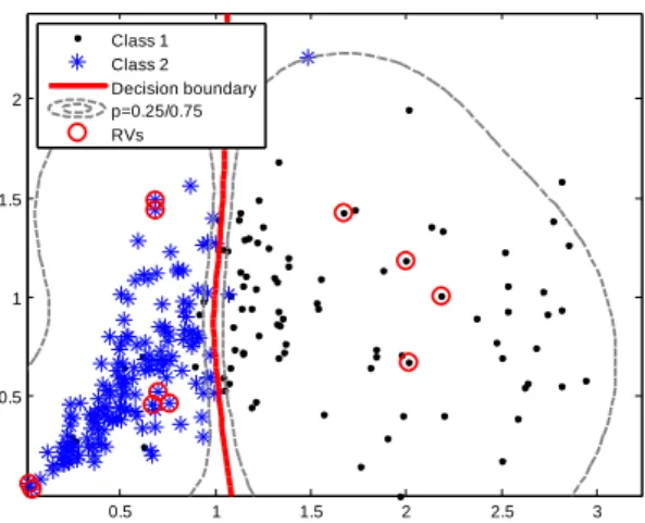
The RV plots for the two class problem{0,1} for the features homogeneity and contrast are shown in Figures1and 2 respectively.

0.2 0.4 0.6 0.8 1 1.2

0.2 0.3 0.4 0.5 0.6 0.7 0.8 0.9 1 1.1 1.2

RVM Classification

Class 1 Class 2 Decision boundary p=0.25/0.75 RVs

Fig. 2. Classification maps obtained for a two-class problem for the feature homogeneity. Red and blue dots indicate the classes {0,1}, red dots point out the relevant vectors (RVs), the red line represents the classification boundary, and the grey lines are the confidence intervals at p = 0.25 and p = 0.75.

MODEL FEATURES AC RV

RVM homogeneity 96 5

(4)

91

0.5 1 1.5 2 2.5 3

0.5 1 1.5 2

Class 1 Class 2 Decision boundary p=0.25/0.75 RVs

Fig. 3. Classification maps obtained for a two-class problem for the feature contrast. Red and blue dots indicate the classes

{0,1}, red dots point out the relevant vectors (RVs), the red line represents the classification boundary, and the grey lines are the confidence intervals at p = 0.25 and p = 0.75.

IV.CONCLUSION

RVM-based image classification provide good classification accuracy, with a significantly smaller RV rate and therefore , much faster testing time.The most evident and compelling results are its accuracy and sparseness .RVM-based classification approach is more suitable for applications that require low complexity and, possibly, real-time classification.

REFERENCES

[1] Pijush Samui1, Venkata Ravibabu Mandla, Arun Krishna and Tarun Teja ―Prediction of Rainfall Using Support Vector Machine and Relevance Vector Machine‖, Open access e-Journal Earth Science India, eISSN: 0974 – 8350 Vol. 4(IV), October, 2011, pp. 188 – 200

[2] A., Chua, L. H. C., and Quek, C. (2010) ―A novel application of a neuro-fuzzy computational technique in event-based rainfall–runoff modeling. Expert Systems with Applications,‖ v. 37(12), pp. 7456–7468.

[3] M. E. Tipping, ―The relevance vector machine,‖ in

Advances in Neural Information ProcessingSystems , vol. 12,

S. A. Solla, T. K. Leen, and K.-R. Müller, Eds. Cambridge, MA: MIT Press, 2000.

[4] M. E. Tipping, ―Sparse Bayesian learning and the relevance

vector machine,‖ J. Mach. Learn. Res., vol. 1, pp. 211–244, 2001.

[5] W. Liyang, Y. Yongyi, R. M. Nishikawa, M. N.Wernick, and A.Edwards,―Relevance vector machine for automatic detection of clustered microcalcifications,‖IEEE Trans. Med.

Imag., vol.24, no. 10, pp. 1278–1285,Oct. 2005.

[6] D. J. C. MacKay, ―The evidence framework applied to Classification networks,‖ Neural Comput., vol. 4, no. 5, pp. 720– 736, 1992.

[7] I.T.Nabney, ―Efficient training of RBF networks for classification,‖ inProc. 9th ICANN, 1999, vol. 1, pp. 210–215.

[8] R.Johansson and P.Nugues, ―Sparse Bayesian classification of Predicate arguments,‖ in Proc. 9th Conf. Comput. Natural Language Learn.,43rd Annu. Meeting Assoc.

Comput. Linguistics, Ann Arbor, MI, 2005,pp. 177–200.

[9] G.Camps-Valls, L.Gomez-Chova, J. Vila-Francés, J. Amorós-López,J. Muñoz-Mar´ı, and J. Calpe-Maravilla, ―Retrieval of oceanic chlorophyll concentration with relevance vector machines,‖ Remote Sensingof Environment, vol. 105, no. 1, pp. 23–33, Nov 2006.

[10] B. E. Boser, I.M. Guyon, and V. Vapnik, ―A training algorithm for optimal margin classifiers,‖ in Proc. 5th Annu.

ACMWorkshop Comput. Learn.Theory, 1992, pp. 144–152.

[11] C. Burges, ―A tutorial on support vector machines for pattern recognition,‖in Proc. Data Miningand Knowl. Discovery,

U.Fayyad, Ed., 1998, pp. 1–43.

[12] F. Melgani and L. Bruzzone, ―Classification of hyper spectral remote sensing images with support vector machines,‖ IEEE Transactions on Geoscience and Remote

Sensing, vol. 42, no. 8, pp. 1778-1790,Aug 2004.

[14] G.Camps-Valls and L. Bruzzone, ―Kernel-based methods for hyper spectral image classification,‖ IEEE

Transactions on Geoscience and Remote Sensing, vol. 43, no.

6, June 2005.

[15] G. Camps-Valls, L. Gómez-Chova, J. Muñoz-Mar´ı, J. Vila-Francés,and J. Calpe-Maravilla, ―Composite kernels for hyper spectral image classification,‖ IEEE Geoscience and

Remote Sensing Letters, vol. 3,no. 1, pp. 93–97, Jan 2006.

[16] Matthias Seeger, ―Gaussian processes for machine learning,‖ International Journal of Neural Systems, vol. 14, no. 2, pp. 69–106, 2004.

[17] C. E. Rasmussen and C. K. I. Williams, Gaussian

Processes for Machine Learning, The MIT Press, 2006.

[18] N. Nikolaev and P. Tino, ―Sequential relevance vector machine earning from time series,‖ in Proceedings of

International Joint Conference onNeural Networks, Montreal,

(5)

92

[19] J. Qui˜nonero-Candela, Learning with Uncertainty –

Gaussian Processes and Relevance Vector Machines, Ph.D.

thesis, Technical University of Denmark, Informatics and Mathematical Modelling, Kongens Lyngby (Denmark), November 2004.

[20] G. Camps-Valls, M. Mart´ınez-Ramón, J. L. Rojo-Álvarez, and J. Muñoz-Mar´ı, ―Nonlinear system identification with composite relevance vector machines,‖

IEEE Sign Processing Letters, vol. 14, no. 4, pp. 279–282, April 2007.

[18] G. Camps-Valls, L. Gomez-Chova, J. Vila-Francés, J. Amorós-López,J. Muñoz-Mar´ı, and J. Calpe-Maravilla, ―Relevance vector machines for sparse learning of biophysical parameters,‖ in SPIE International Symposium Remote

Sensing, XI, Bruges, Belgium, Set 2005, vol. 5982.

[19] G.Camps-Valls, L. Gomez-Chova, J. Vila-Francés, J.Amorós- López,J. Muñoz-Mar´ı, and J. Calpe-Maravilla, ―Retrieval of oceanic chlorophyll lconcentration with relevance vector machines,‖ Remote Sensingof Environment, vol. 105, no. 1, pp. 23–33, Nov 2006.

Kalarani Athilingam completed her B.Engg. degree in Electronics and Communication Engineering from Anna University, Chennai, in 2008 and the Master of Engg. degree from Anna University, Tirunelveli, in 2010. From June 2010 to till now, She is working in P.S.R.Rengasamy College of Engg for women, Sivakasi. Her research area includes Digital Electronics, Digital Image processing, Antenna. Communication theory.She has been attended several workshops and conferences in various engg colleges.

Viji Gurusamy received the B.Engg. degree in Electronics and Communication Engineering from Anna University, Chennai, in 2008 and the Master of Engg. degree from Anna University, Thirunelveli, in 2010. From June 2010 to May 2012, She was worked in M.Kumarasamy College of Engg, Karur. Now she is currently working in P.S.R.Rengasamy College of Engg for women, Sivakasi. She had attended four international conferences and one national conference in various colleges. Her research area includes Digital Signal processing, Digital Image processing, Digital Communication.