THE CORRELATION ANALYSIS OF THE SHAPE PARAMETERS FOR ENDOTHELIAL IMAGE CHARACTERISATION

THE CORRELATION ANALYSIS OF THE SHAPE PARAMETERS FOR

ENDOTHELIAL IMAGE CHARACTERISATION

K

N

B

A

P

1_{Institute of Informatics, Faculty of Automatic Control, Electronics and Computer Science, Silesian University}

of Technology, ul. Akademicka 16, 44-100 Gliwice, Poland;2AGH University of Science and Technology, Departament of Geoinformatics and Applied Computer Science, Cracow, Poland.

e-mail: [email protected], [email protected]

(Received May 23, 2016; revised October 5, 2016; accepted October 20, 2016)

ABSTRACT

Microscopic images of corneal endothelium cells are investigated to deliver information about their medical state. Although this could be achieved automatically, this examination is manual and very time consuming. Two medical parameters for endothelial layer quality description have been introduced and more are planned. Yet, since they will exploit image processing, a thoughtful overview of applicable existing shape parameters is necessary. This work investigates the possibility of exploiting well-known image processing techniques for describing the endothelial layer by calculating information about shape features using spatial moments or topological attributes. The comparison concentrates on finding which shape measures could be combined to improve descriptions, and which cannot due to their high correlation and the fact that they do not contain any new information. The performed experiments revealed a set of 17 non-correlated features and four groups of shape parameters that show some correlation, but one representative can always be selected. Moreover, the investigation proved some correlation between the metrics used in medicine and considered shape features. Keywords: correlation analysis, endothelial images, shape parameters.

INTRODUCTION

The corneal endothelium is the translucent frontal part of the eyeball which is responsible for keeping the cornea clear by draining water from it (Agarwalet al., 2002). It is a monolayer of cells whose shape in healthy structures reflects a hexagon. The number of corneal endothelium cells at birth is around 6,500 cells/mm2, decreasing to 1,700–2,000 cells/mm2at the age of 80, as reported by Koet al.(2000; 2001), because the cells do not reproduce (Meyer et al., 1988). When a cell dies, neighboring cells grow and take its place to fill the layer tightly. Their shape changes as a result.

The structure, number, and composition of cells in the endothelial layer are observed in vivo by non-contact specular microscopy or inverse phase contrast microscopy. The shape and spatial distribution reflect the state of the corneal endothelium after surgical procedures and are basic information for a physician. Although manual annotation of this data is not a problem, it is tiresome work. Therefore, several automatic and semi-automatic solutions for endothelial cell location were developed (Meijering, 2012).

DETERMINATION OF CELL LOCATION

Although precise determination of cell location in endothelial images seems simple, it proved to be

a difficult task for a computer program due to the irregular illumination and artefacts caused by high amounts of noise and distortion, as indicated by Gavet and Pinoli (2008). Initial solutions tend to deal with all problems altogether as present works by Nadachi and Nunokawa (1992); Vincent and Masters (1992); Hasegawa et al. (1996); Mahzoun et al. (1996); Foracchia and Ruggeri (2000); Serra and Mlynarczuk (2000).

Yet, the trend in algorithm design later changed, when issues concerning accurate location of endothelial cell borders were well defined. Therefore, three stages are clearly noticeable in recently introduced solutions. The first stage is responsible for illumination compensation and noise removal. Some interesting ideas can be found in works by Sanchez-Marin (1999); Habratet al.(2016).

Bayesian framework supported by simulated annealing for cell border location (Foracchia and Ruggeri, 2003) improved by statistical description (Foracchia and Ruggeri, 2007); exploiting active contours (Dagher and El Tom, 2008), snake-lets (Charłampowiczet al., 2014), level sets (Zhou, 2007), and wavelets (Khan et al., 2007). The data mining and rough sets theory found an application in the solution designed by Poletti and Ruggeri (2014); while Ruggeri et al.(2010) used an artificial neural network to classify whether a pixel belongs to a cell body or boundary oriented at different angles; the genetic algorithm was exploited by Ruggeri and Scarpa (2015); Scarpa and Ruggeri (2015), who supported it with information about pixel intensities and regularity of cell shapes. Finally, the third stage is thinning, which is used to locate cell borders precisely. Saeed et al. (2010) introduced the K3M algorithm for image skeletonization. Recently, a very interesting comparison that paid attention to cell border determination accuracy and the influence on parameter calculation of a repeatability framework was presented by Piorkowskiet al.(2016).

EXISTING MEDICAL PARAMETERS

Images of the corneal endothelium with marked cell borders are insufficient for a physician. An automatic method for comparison and endothelial layer state description is necessary in order to support tracking of endothelial structure changes due to ageing or damage caused by disease or surgical procedures.

Straightforward comparison of a grid which represents cell borders is impossible, because available distance metrics do not correspond to the way humans interpret images, as described by Gavet and Pinoli (2013). Therefore, in medicine, for each cell, a shape parameter value is calculated and the image content is described using a statistical approach that exploits this data.

Historically, Rao et al. (1982) introduced calculation of the size of cells recorded in the image first. Next, Doughty (1990) described a coefficient of variation that describes changes in cell area size in images, and later Doughty (1992) discussed the hexagonality measure, which is understood as the probability of finding a hexagonal cell in the image. Ollivier et al. (2003) proved that these parameters are likely to describe endothelial layer function, because the researchers noticed that size distribution varies between healthy and pathological tissues. Gronkowska-Serafin and Piorkowski (2014) introduced a novel parameter that describes the average coefficient of variation of cell side lengths and Piorkowski et al. (2015) proved its high stability compared to previous cell shape parameters.

Another approach to cell shape description presents a granulometric measure that assumes that cell shape is related to a disk, and therefore includes in calculations cells that are only partially visible in the image. Thanks to this assumption, it is possible to estimate the radius of each cell, which part was detected in the image (usually on its boundary) and consider its area in calculations. In this case, Ayala et al. (2001) suggested using a probability density function, while granulometric moments were exploited by Zapteret al.(2005) for data description. According to D´ıazet al.(2007), this manner of endothelial image description is better because it combines information about size, shape, and spatial distribution. There are also approaches which exploit fractal dimensions for nuclei description (Oszutowska-Mazureket al., 2012; 2013; 2015), but they have not find an application in endothelial image analysis yet.

RESEARCH OBJECTIVES

Researchers who design medical parameters concentrate on features that are considered during the visual inspection of data. This approach appears to be valid; however, in reality it is unknown how shapes are compared by humans. Moreover, adapting human thinking when preparing an algorithm for a computer may be misleading.

This work addresses the problem of shape description for endothelial cells. Since we are working with digital data, a plethora of object shape features known from the image processing domain may find an application and create a perfect image content descriptor. Such parameters should make it possible to differentiate between healthy and pathological endothelial layer structures, and should give similar results irrespective of the cell border determination method applied. Therefore, this work compares its descriptive qualities, searches for possible correlation in order to chose such parameters, which application gives new and broad data description removing unnecessary redundancy. Additionally, the overview of the broad range of existing parameters should give a better insight into endothelial cell shape characteristics and in the future may lead to a better understanding of shape changes.

presented in section Results section Discussion discusses the results and draws the conclusions.

MATERIAL AND METHODS

MEDICAL PARAMETERS

As was stated in section Existing Medical Parameters, two groups of parameters are considered for describing the shape of endothelial cells. The first examines cell shape characteristics and is already used in medicine (Raoet al., 1982; Doughty, 1990; 1992). The second is a granulometry measure (Ayala et al., 2001; Zapteret al., 2005; D´ıazet al., 2007) which, to the best our knowledge, did not find an application. Therefore, the second approach is not included in this research.

The most common endothelial cell descriptor used in medicine is the cell densityCD measure. It correlates the average cell size to the total investigated area. This parameter is automatically calculated by the TOPCON software, therefore became widely exploited.

A coefficient of variation in the area size of different cells was described by Doughty (1990). It measures cell size distribution over the whole population and usually has a value below 30% for healthy structures. It is defined as follows:

CV= 1 µc s 1 N N

∑

i=1

(ci−µc)2·100%, (1)

whereciis the area ofith cell,µcis the average area of

cells in the image, andN is the number of cells. This formula is a general statistical method, which enables describing the data standard distribution in population and can be applied to any other measure.

The hexagonality coefficient H was discussed by Doughty (1992) and calculates the proportion of hexagonal cells (N6) to those of other shapes (NT)

following the equation:

H= N6

NT

·100%. (2)

This measure states the proportion of cells with hexagonal shape, has a value above 50% for healthy structures, and decreases with age.

The coefficient of cell side length variation CVSL was introduced by Gronkowska-Serafin and Piorkowski (2014) and is given as:

CVSL= 1

N

N

∑

j=1 1 ¯ SLj v u u t 1 NLj NL_j

∑

i=1

(li−SL¯ j)2, (3)

whereliis the length of theith side of the jth cell, ¯SLj

is the average length of all sides of jth cell andNLj

is the number of sides and N is the number of cells. This parameter is sensitive to deformation of cells, especially for stretching.

SHAPE PARAMETERS

Several techniques have been developed in order to describe the shape of objects presented in binary images. Some of them exploit topological information about pixel distribution within the object; others describe its statistical qualities. In this work, both approaches have been used and their accuracy for the description of endothelial image content has been evaluated.

Spatial moments

A probability theory concerning spatial moments was adopted by Gonzalez and Woods (2001) to describe binary images, especially the shape of objects. In this approach, an imageIis understood as a discrete function I(x,y), where pixels describing the object have ones as values and the background is marked with zeros. The summation over such defined function enables to define the spatial momentSMof the(m,n)th order as follows:

SMm,n=

1 Wm_·Hn

W

∑

x=1

H

∑

y=1

xm·yn·I(x,y), (4)

where x and y are coordinates of pixels in image, andW andH are the width and height of the image, respectively. Usually, moments of the following orders are considered: (0,0); (1,0); (0,1); (2,0); (1,1);

(0,2); (3,0); (2,1); (1,2); (0,3). This formulation assumes that the origin of coordinates is in the lower left corner of an image, and the first factor in Eq. 4 removes scaling dependency from the spatial moment calculation. The derived moments have several properties, for example the SM₀,0 describes object area and the relation betweenSM1,0 andSM0,0, andSM0,1andSM0,0makes it possible to calculate the objects center of gravity(x¯,y¯).

If the centroid of the object is known, it is possible to derive spatial central momentsCM:

CMm,n=

1 Wm_·Hn

W

∑

x=1

H

∑

y=1

(x−x¯)m·(y−y¯)n·I(x,y) (5)

and spatial normalized central moments NM, additionally prone to scale variations:

NMm,n=

CMm,n

SM

m+n

2 +1

0,0

The last moments were introduced by Hu (1962), who used them to derive seven invariant moments IM, whose values do not change under translation, rotation, and scaling of the object.

Topological attributes

Shape parameters based on topology are not affected by translation and rotation. Several definitions are given by Gonzalez and Woods (2001); Russ (1998); Jahne (2002). In a binary image, the area and perimeter are the basic shape characteristics of the object. The area Acounts pixels which belong to the object, whereas the perimeter P is defined as the number of pixels which belong to the object, but are placed on its boundary.

With information about area and perimeter of an object, several geometric measures are defined which are not affected by rotation, translation, and changes of scale. Several of them are the circularity measurements, which are given by different formulas:

C1=

4·π·A

P2 , (7)

C2= P2

A , (8)

C3=

2·π·A

P , (9)

Malinowska= P

2√π·A

−1, (10)

Shapeless= P

2

4·π·A . (11)

TheC1,C2,C3, and “Shapeless” result in unity value for circular shapes, while “Malinowska” has a zero value. The greater the variation from unity (or zero), the more elongated and complex a shape is. There are also other parameters concerning circularity:

C4= P

π , (12)

C5= AMAX

P , (13)

Roughness=2·

r A

π , (14)

where AMAX is the maximal area calculated as the

multiplication of maximal width and height of object.

Other definitions calculate the elongation of object as the ratio between the maximum diameters D orthogonal to each other:

Feret= DI

DII

. (15)

There are also several complex parameters that except object’s area use information about distribution of the shortest distancessdbetween each of the objects pixels and the contour:

Blair-Bliss=q A 2·π·∑isdi2

, (16)

Danielsson= A

3

(∑isdi)2

. (17)

Other parameters focus the calculation on the distances d between the points on the contour and the center of gravity of the object:

Haralick=

s

(∑idi)2

P·∑idi2−1

. (18)

Another parameter expresses the ratio between the largest and smallest distance of contour points of the object to its center of gravity (PD):

W7= minPD

maxPD. (19)

For each shape parameter, the value describing the whole image was calculated following the Eq. 1, where pstands for chosen parameter value andµp for

its average:

Param= 1 µp

s 1 N

N

∑

i=1

(pi−µp)2. (20)

This approach, which calculates general standard deviation of each parameter, has been chosen as an objective mean for descriptive parameter values comparison.

EXPERIMENTAL DATA

The experimental data set was acquired with an inverse phase contrast microscope (CK 40, Olympus) at 200×magnification and an analogue camera (SSC-DC50AP, Sony) by Ruggeri et al. (2010). The set consists of 30 images of a corneal endothelium taken from 30 porcine eyes stained with alizarine. The images are monochromatic in JPEG format at 768×

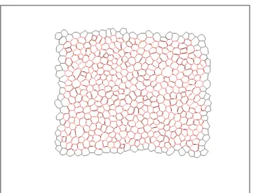
(a) Example of input data

(b) Original cell borders (c) Thinned cell borders

Fig. 1. Exemplary image of endothelial layer with marked cell borders: (b) existing in the data set; (c) thinned for calculation.

Table 1.Masks set used for thinning. X denotes pixels not included in the square mask.





X 1 1

0 1 1

0 0 X



 



1 1 1

0 1 0

0 0 0



 



X 1 X X 1 X

0 0 0









X X 0

0 1 0

0 0 0



 



0 X X

0 1 0

0 0 0





Except for original endothelial layer images, the dataset contains manually prepared segmentations in seed form. This means that cell borders are thicker than 1 pixel. Therefore, before information about cell shapes can be acquired, thinning was necessary. The skeletonization procedure was performed using all masks from the set masks shown in Table 1 with orientations: 0◦, 90◦, 180◦, and 270◦.

Fig. 2. Original cell borders for Fig. 1a with additionally marked in red thinned locations of cells considered for calculation in order to assure information about cell sides.

The thinning procedure was sufficient in order to determine the shape parameters, but in the case of H and CV SL metrics, some additional processing was necessary. The computation of this cell feature is strongly related to its neighbors, due to the information about number and length of cell sides; therefore, using the data prepared by the authors of the dataset would result in unreliable results for all cells on the region border. In order to meet the demands and assure that for each cell there is information about how many sides it has, we decided to remove from the whole computations the first envelop of cells, which lacks such information, as is depicted in Fig. 2. Moreover, the black lines correspond to the skeletonized cell borders calculated from original data, whereas the red lines approximate straight connections between nodes (tripple points) calculated in the points where three sides were crossing. This approximation is necessary for correct computation ofHandCV SLparameters.

Table 2.Absolute correlation value range for a group name.

Name Min Max

Perfect 0.99 1.00

Very good 0.95 0.98

Good 0.90 0.94

Possible 0.80 0.89

Satisfactory 0.70 0.79

Weak 0.50 0.69

None 0.00 0.49

RESULTS

The goal of this experiment was to find which of the presented parameters are correlated and therefore should not be used together to describe the endothelial layer image content. Using such parameters in sets to describe the data should be avoided, as they do not convey any additional information.

In order to calculate the correlation measure for each testing image, the cell boundaries were located, then a chosen parameter was calculated for each cell in the image and the final value was obtained following Eq. 20. These values were used to calculate the correlation.

When plotting all calculated correlation values on one graph it turned out that there are three aggregations of correlated parameters between each other only and several correlated pairs of features. Since presenting a plot with 55 features is impossible, the authors decided to present each aggregations on separate plots. Therefore, the following figures depict groups correlated together. However, for interested reader the matrix presenting all correlation values is accessible as a supplementary file.

DISCUSSION

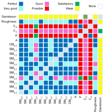
Fig. 3 shows Group I of features, which are characterized in most cases by very good or perfect correlation. This group consists of 17 features. It is not surprising to see that A, SM0,0, and CM0,0 are very strongly correlated, as all these measures define the area of an object. Next, good or better correlation was recorded between all possible orders of SM. Then, several shape parameters (A, P, C3, C4, and “Roughness”) reported satisfactory or better correlation. Finally, a weak correlation with “Danielsson” feature was noticed.

Fig. 3. Group I of features with almost perfect correlation.

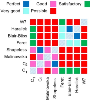
Group II presented in Fig. 4 only consists of shape parameters whose correlation is in most cases above the possible range. A good correlation between C₁, C₂, “Malinowska”, “Shapeless” was suspected as all of these features are a scaled or inverse of relation P2/A. However, it is interesting to see that they do not show correlation with others circularity measures, which belong to Group I. Next, the perfect correlation between “Blair-Bliss” and “Haralick” is also interesting as these measures are calculated using different shape properties. The “Feret” feature behaves similarly to the aforementioned features.

Fig. 5 groups features for which the correlation from weak to possible range was calculated: Group III. Except for one very good correlation betweenNM0,1 andIM₁, the other features proved to be less related to each other. It is interesting to find that such a simple measure asC5is correlated with the statistical features presented in this group. The correlation between others probably results from common parts in the formula definition.

Finally, Group IV consists of pairs of features:

– IM5andIM6which are possibly correlated,

– CM₁,0andNM1,0which are satisfactory correlated,

– CM0,2andNM0,2which are satisfactory correlated,

Fig. 4.Group II of shape features with at least possible correlation.

Fig. 5. Group III of features with at least weak correlation.

The correlation value presented and discussed above is not sufficient to verify whether correlation between two datasets exists. It is necessary to plot the data and see whether the trend is visible. For each pair of features, such a scatter-plot was prepared and checked. The examples of data distribution showed that the calculated correlation corresponds well to the plots. Moreover, when the results of correlation plots for different groups were compared, it was seen how the distribution varies more in two dimensions when

the correlation value lowers. In almost all cases, a positive correlation took place, only for pairs with “Malinowska” was a negative correlation recorded.

Additionally, for each pair of features the p-value was calculated to verify a null hypothesis that the data describing two features comes from independent random samples. Values lower than the significance level set to 0.05 allow to reject this hypothesis for all elements in Group II and most in Group III (except three pairs consisting of Shapeless,C1, andC2). In case of Group I, the hypothesis is rejected for pairs created from “Danielsson”, “Roughness” (except pair with C3),C4(except pair withP),C3, andP. In other cases there are no bases to reject the hypothesis. Considering Group IV the hypothesis can be rejected for IM₅ and IM6pair as well as forCM21andNM2,1.

From the presented experiment and the gathered data, one can conclude that it is possible to distinguish several endothelial layer descriptive features that are not correlated to each other. Moreover, it is possible to choose one representative from those correlated to be used to describe the data. Table 3 names the non-correlated and chosen representatives, which are characterized by at least possible correlation value.

The next experiment assumed calculation of correlation between parameters used in medicine (CD, CV,CV SL, andH) and those discussed in the previous experiment. It was found out that, since the method for parameter calculation was derived fromCV definition, it behaves asAbecause its calculation is similar. Next, theCV SLparameter proved to have weak correlation with features considered in Group II. Only theCDand Hfeatures are not correlated to any other features.

Table 3.Not correlated features. Features marked by∗ have very low correlation which exists only between two measures, hence it was decided to join them to non-correlated group.

Features

Group I A

Group II C₂

Group III CM0,1

Group IV IM5

Non-correlated IM₇

This article investigates the shape parameters used in the image processing domain as a means for endothelial image description. The main objective of the presented experiments is to verify which parameters should be considered for such data descriptions, and which could improve understanding and support automatic analysis of endothelial images. It was very important to remove the information redundancy that exists in correlated measures.

According to the performed experiments that addressed the spatial moments and topological attributes, there are four groups of features correlated to each other, but also 17 non-correlated metrics were distinguished. From each group, a representative with the lowest computation overload was suggested for further consideration. Additionally, it was found that the medical parameterCV andCVSLare correlated to a group of features, whileCDandH does not exhibit such properties.

In further research, application of chosen shape features for differentiation between healthy and damage tissue will be considered. Moreover, the accuracy of endothelial image quality description with these features will be investigated.

ACKNOWLEDGEMENTS

K. Nurzynska was supported by statutory funds for young researchers (BKM/507/RAU2/2016) of the Institute of Informatics, Silesian University of Technology, Poland. A. Piorkowski was financed by the AGH – University of Science and Technology, Faculty of Geology, Geophysics and Environmental Protection as a part of statutory project.

REFERENCES

Agarwal S, Agarwal A, Apple D, Buratto L (2002). Textbook of ophthalmology, vol. 2. New Dehli: Jaypee Brothers, Medical Publishers Ltd.

Ayala G, Diaz M, Martinez-Costa L (2001). Granulometric moments and corneal endothelium status. Pattern Recogn 34:1219–27.

Bernander KB, Gustavsson K, Selig B, Sintorn IM, Luengo Hendriks CL (2013). Improving the stochastic watershed. Pattern Recogn Lett 34:993–1000.

Caetano CAC, Entura L, Sousa SJ, Tufo REA (2000). Identification and segmentation of cells in images of donated corneas using mathematical morphology. In: Proc XIII IEEE Brazil Symp Comput Graph Image Proc 344

Charłampowicz K, Reska D, Boldak C (2014). Automatic segmentation of corneal endothelial cells using active contours. Adv Comp Sc Res 11:47–60.

Dagher I, El Tom K (2008). Waterballoons: A hybrid watershed balloon snake segmentation. Image Vision Comput 26:905–12.

D´ıaz ME, Ayala G, Sebastian R, Mart´ınez-Costa L (2007). Granulometric analysis of corneal endothelium specular images by using a germ–grain model. Comput Biol Med 37:364–75.

Doughty M (1990). The ambiguous coefficient of variation: Polymegethism of the corneal endothelium and central corneal thickness. Int Contact Lens Clinic 17:240–8. Doughty M (1992). Concerning the symmetry of the

hexagonal cells of the corneal endothelium. Exp Eye Res 55:145–54.

Foracchia M, Ruggeri A (2000). Cell contour detection in corneal endothelium in-vivo microscopy. In: Proc 22nd IEEE Ann Int Conf Eng Med Biol Soc (EMBS) 2:1033– 5.

Foracchia M, Ruggeri A (2003). Corneal endothelium analysis by means of bayesian shape modeling. In: Proc 25th IEEE Ann Int Conf Eng Med Biol Soc (EMBS) 794–7.

Foracchia M, Ruggeri A (2007). Corneal endothelium cell field analysis by means of interacting bayesian shape models. In: Proc 29th IEEE Ann Int Conf Eng Med Biol Soc (EMBS) 6035–8.

Gavet Y, Pinoli JC (2008). Visual perception based automatic recognition of cell mosaics in human corneal endotheliummicroscopy images. Image Anal Stereol 27:53–61.

Gavet Y, Pinoli JC (2013). Human visual perception and dissimilarity. SPIE Newsroom 10.1117/2.1201311.004338

Gonzalez RC, Woods RE (2001). Digital image processing. Boston, MA, USA: Addison-Wesley Longman Publishing Co., Inc., 2nd ed.

Gronkowska-Serafin J, Piorkowski A (2014). Corneal endothelial grid structure factor based on coefficient of variation of the cell sides lengths. In: Image processing and communications challenges 5, Adv Intel Syst Comput 233:13–9.

Habrat K, Habrat M, Gronkowska-Serafin J, Piorkowski A (2016). Cell detection in corneal endothelial images using directional filters. In: Image processing and communications challenges 7, Adv Intel Syst Comput 389: 113–23.

Hasegawa A, Itoh K, Ichioka Y (1996). Generalization of shift invariant neural networks: image processing of corneal endothelium. Neural Networks 9:345–56. Hu MK (1962). Visual pattern recognition by moment

Jahne B (2002). Digital image processing: concepts, algorithms, and scientific applications, 5th ed. Secaucus, NJ, USA: Springer.

Khan MAU, Niazi MKK, Khan MA, Ibrahim MT (2007). Endothelial cell image enhancement using non-subsampled image pyramid. Inform Technol 6:1057– 62.

Ko M, Lee J, Chi J (2000). Cell density of the corneal endothelium in human fetus by flat preparation. Cornea 19:80–3.

Ko M, Park W, Lee J, Chi J (2001). A histomorphometric study of corneal endothelial cells in normal human foetuses. Exp Eye Res 72:403–9.

Latała Z, Wojnar L (2001). Computer-aided versus manual grain size assessment in a single phase material. Mater Charact 46:227–33.

Mahzoun M, Okazaki K, Mitsumoto H, Kawai H, Sato Y, Tamura S, Kani K (1996). Detection and complement of hexagonal borders in corneal endothelial cell image. Med Imaging Technol 14:56–69.

Malmberg F, Selig B, Luengo Hendriks C (2014). Exact evaluation of stochastic watersheds: From trees to general graphs. In: Barcucci E, Frosini A, Rinaldi S, Eds. Discrete geometry for computer imagery. Lect Not Comput Sci 8668: 309–19.

Meijering E (2012). Cell segmentation: 50 years down the road [life sciences]. IEEE Signal Proc Mag 29:140–5. Meyer L, Ubels J, Edelhauser H (1988). Corneal endothelial

morphology in the rat. Invest Ophthalmol Vis Sci 29:940–9.

Nadachi R, Nunokawa K (1992). Automated corneal endothelial cell analysis. In: Proc 5th Ann IEEE Symp Comput Med Syst 450–7

Ollivier F, Brooks D, Komaromy A, Kallberg M, Andrew S, Sapp H, Sherwood M, Dawson W (2003). Corneal thickness and endothelial cell density measured by non-contact specular microscopy and pachymetry in Rhesus macaques (Macaca mulatta) with laser-induced ocular hypertension. Exp Eye Res 76:671–7.

Oszutowska-Mazurek D, Mazurek P, Derda K, Sycz K, Waker-W´ojciuk G (2015). Sensitivity of nuclear-cytoplasmic index and nuclear-nuclear-cytoplasmic relation in computer aided cytoscreening diagnosis. Prz Elektrotechn 91:56–8.

Oszutowska-Mazurek D, Mazurek P, Sycz K, Waker-W´ojciuk G (2012). Estimation of fractal dimension according to optical density of cell nuclei in Papanicolaou smears. In: Information Technologies in Biomedicine, Lect Not Comput Sci 7339:456–63. Oszutowska-Mazurek D, Mazurek P, Sycz K,

Waker-W´ojciuk G (2013). Variogram based estimator of fractal dimension for the analysis of cell nuclei from the

papanicolaou smears. In: Image Proc Commun Chal 4. Adv Intel Syst Comput 184:47–54.

Piorkowski A, Gronkowska-Serafin J (2015). Towards precise segmentation of corneal endothelial cells. In: Bioinformatics and Biomedical Engineering, Lect Not Comput Sci 9043:240–9.

Piorkowski A, Mazurek P, Gronkowska-Serafin J (2015). Comparison of assessment regularity methods dedicated to isotropic cells structures analysis. In: Image Proc Commun Chal 6, Adv Intel Syst Comput 313:169–78.

Piorkowski A, Nurzynska K, Gronkowska-Serafin J, Selig B, Boldak C, Reska D (2016). Influence of applied corneal endothelium image segmentation techniques on the clinical parameters. Comp Med Imaging Graphics (in press) DOI: 10.1016/j.compmedimag.2016.07.010 Poletti E, Ruggeri A (2014). Segmentation of corneal

endothelial cells contour through classification of individual component signatures. In: Proc XIII Mediter Conf Med Biol Eng Comput 2013. IFMBE Proc 41:411–4.

Rao GN, Lohman L, Aquavella J (1982). Cell size-shape relationships in corneal endothelium. Invest Ophthal Vis Sci 22:271–4.

Ruggeri A, Scarpa F (2015). Computerized analysis of human corneal endothelium morphology. Acta Ophthalmol 93:ABS15-0551.

Ruggeri A, Scarpa F, De Luca M, Meltendorf C, Schroeter J (2010). A system for the automatic estimation of morphometric parameters of corneal endothelium in alizarine red stained images. Br J Ophthalmol 94:643– 7.

Russ J (1998). The Image Processing Handbook, 3rd Ed. Boca Raton: CRC Pres.

Saeed K, Tabe¸dzki M, Rybnik M, Adamski M (2010). K3M: A universal algorithm for image skeletonization and a review of thinning techniques. Int Appl Math Comp 20:317–35.

Sanchez-Marin F (1999). Automatic segmentation of contours of corneal cells. Comput Biol Med 29:243–58. Scarpa F, Ruggeri A (2015). Segmentation of corneal endothelial cells contour by means of a genetic algorithm. In: Proc 2nd Int Worksh Ophtal Med Image Anal 4:25–32.

Selig B, Malmberg F, Luengo Hendriks CL (2015a). Fast evaluation of the robust stochastic watershed. In: Mathematical morphology and its applications to signal and image processing. Lect Not Comput Sci 9082:705– 16.

confocal microscopy. BMC Med Imaging 15:13. Serra J, Mlynarczuk M (2000). Morphological merging of

multidimensional data. Proc STERMAT 2000, 385–90. Vincent LM, Masters BR (1992). Morphological image processing and network analysis of cornea endothelial cell images. In: Image Algebra Morphol Image Proc III. Proc SPIE 1769:212–26.

Zapter V, Martinez-Costa L, Ayala G (2005). A granulometric analysis of specular microscopy images of human corneal endothelia. Comp Vis Image Und 97:297–314.