An Agile and Robust Sparse Recovery Method for MR Images Based on Selective k-space Acquisition and Artifacts Suppression

(1)

Vol.2 No.2, 2018

http://innove.org/ijist/ 3

An Agile and Robust Sparse Recovery Method for MR

Images Based on Selective k-space Acquisition and

Artifacts Suppression

Henry Kiragu, Elijah Mwangi and George Kamucha School of Engineering

University of Nairobi

P.O. BOX 30197-00100, Nairobi, Kenya. [email protected]

Abstract—Magnetic Resonance Imaging (MRI) has some attractive advantages over other medical imaging techniques. Its widespread application as a medical diagnostic tool is however hindered by its long acquisition time as well as reconstruction artifacts. A proposed Compressive Sampling (CS) based method that addresses the two limitations of conventional MRI is presented in this paper. The proposed method involves acquisition of an under-sampled k-space by employing a smaller number of phase encoding gradient steps than that dictated by the Nyquist sampling rate. The MR image reconstructed from the under-sampled k-space is then randomly sampled and reconstructed using a greedy sparse recovery method in the wavelet domain. To improve the robustness of the method, a proposed high-pass filter is used to suppress the reconstruction artifacts. The Peak Signal to Noise Ratio (PSNR) as well as the Structural SIMilarity (SSIM) measures are used to assess the performance of the proposed method. Computer simulation results demonstrate that the proposed method reduces the reconstruction concomitant artifacts by 1.75 dB for a given CS percentage measurement. For a given output image quality, the proposed method gives a scan time reduction of 20%.

Index Terms— Compressive sampling, concomitant artifacts, acquisition time, magnetic resonance imaging.

I. INTRODUCTION

For a band-limited continuous-time signal to be recoverable from its samples, it should be sampled at a rate that is at least twice its highest frequency

component. This signal acquisition paradigm is in accordance to the Shannon-Nyquist sampling theorem. Applying the theorem to the acquisition of some high dimensional signals such as in Magnetic Resonance Imaging (MRI) leads to an excessively long acquisition time. However, if the signal is

sparse or compressible in some suitable

representation domain, the long acquisition time can be reduced by taking measurements that are highly incomplete according to the Shannon-Nyquist sampling theorem. The signal can then be reconstructed from the measurements using sparse reconstruction methods. This signal acquisition and recovery approach is referred to as Compressive Sampling (CS). The signal acquisition stage of CS combines the sensing and compression stages of traditional signal acquisition approaches into a single step. Application of the CS theory in the acquisition and reconstruction of signals is only successful if the signal plus the measurement procedure used meet some requirements. In addition to the signal being sparse or compressible in a

suitable representation domain, the signal

measurement and representation methods must be highly incoherent. The signal acquisition process can be modeled as a multiplication of the signal by a rank-deficient measurement matrix to produce a measurement vector. On the other hand, the sparse domain representation of the signal is equivalent to a

multiplication of the signal by a square

representation matrix. The product of the two matrices yields the CS sensing matrix. For the incoherence condition to be met, the maximum

cross-correlation between the rows of the

(2)

Vol.2 No.2, 2018

individual columns of the sensing matrix. The number of measurements required to accurately reconstruct the sparse signal is directly proportional to the square of the coherence between the measurement and the representation matrices. The sensing matrix must also possess the Restricted Isometry Property (RIP). The RIP condition ensures that the Euclidean separations between signals of interest are preserved in the representation domain. This separations preservation ensures unique reconstruction of all the signals of interest from their CS measurement vectors [1][2][3][4]. Although some deterministic matrices satisfy the RIP requirement, they require a special design of the measurement matrix and also lead to a requirement of a measurement vector that is unacceptably large. These limitations of the deterministic sensing matrices are overcome by using random matrices whose entries are independent and identically distributed entries picked from a continuous sub-Gaussian distribution. The methods used to reconstruct the sparse signal from its CS measurement vector include optimization, iterative and thresholding methods [4][5][6].

Magnetic Resonance Imaging (MRI) is a medical diagnostic technique that has some outstanding merits compared to other clinical imaging modalities. The method is non-invasive since it does not require any surgical intervention in order to image the interior of a human body as opposed to methods such as intravascular ultrasound and catheter venography. The Radio Frequency (RF) excitation pulses employed in MRI are incapable of causing ionization in the body tissues as opposed to the x-rays utilized in Computed Tomography (CT). Therefore, MRI does not put the patient at the risk of developing cancer due to prolonged exposure. Magnetic Resonance (MR) images have better soft-tissue contrast than CT images. In addition, MRI systems have parameters such as the gradient echo time (TE), the spin-lattice relaxation time constant (𝑇1) and the spin-spin relaxation time constant (𝑇₂) that can be exploited to flexibly change the image contrast. Whereas CT imaging uses iodine-based contrast agents, MRI uses gadolinium-iodine-based ones. The iodine-based contrast agents can trigger allergic reactions in some patients unlike the

gadolinium-based ones. Despite the many

advantages, MRI is characterized by long scan times. This is partially as a result of the large sequence repetition time (TR) required to allow the flipped spins to relax to their equilibrium state with

relaxation time constant 𝑇₁. Another factor

contributing to the long scan time is the large number of phase encoding steps required to meet the Shannon-Nyquist sampling criterion. The long MR imaging time makes it difficult for many patients to remain motionless in the MRI equipment. In addition, MR images are usually degraded by equipment-related as well as patient-related artifacts. The artifacts are as a result of non-idealities in the MRI equipment and voluntary as well as involuntary motions of the patient’s body [7][8][9][10].

Magnetic resonance images are usually sparse or compressible in the Discrete Wavelet Transform (DWT) or the Discrete Fourier Transform (DFT) domains. The problem of long image acquisition time experienced in MRI can therefore be solved using CS methods [11][12][13].

Vellagoundar and Reddy have proposed a CS-based method for reconstructing MR images from their under-sampled k-space data [14]. The method generally produces images of good quality. However, when the measurement vector has a length of about one-eighth of the low-frequency region of the k-space, the reconstructed MR images reveal artifacts in the phase-encoding direction. These artifacts compromise the quality of the reconstructed images and can result in misleading diagnosis of a medical condition. The CS-MRI algorithm proposed in [15] exploits the image sparsity and the characteristic profile of the image coefficients in the

wavelet transform domain. The images

(3)

Vol.2 No.2, 2018

reconstruction algorithm reported in [17] gives recovered images that have good edges and few artifacts. This method appears to have high computational complexity due to use of the complex double-density dual-tree DWT. The method is therefore not suitable for real time imaging.

In this paper, an algorithm for acquisition and reconstruction of MR images using CS techniques is proposed. The procedure involves selective k-space

acquisition, random sampling, greedy CS

reconstruction in the DWT domain and finally DFT domain denoising to suppresses the concomitant artifacts. The method is characterized by low scan time, high quality images and low computational complexity since it uses a simple modified high pass filter and does not require adjustment of parameters for images of different sizes.

The remainder of this paper is arranged as follows. Section II gives a brief background theory on CS, MRI and image quality metrics. The proposed algorithm is presented in section III while section IV presents the MATLAB simulation experimental results. In section V, a conclusion and suggestions for further work are given.

II. THEORETICAL BACKGROUND This section outlines the requisite theory that is applied in the paper. The section covers compressive sampling, magnetic resonance imaging and image quality metrics theories.

A. Compressive sampling theory

Using Compressive Sampling (CS) theory, the acquisition of a high-dimensional signal is done by taking measurements that are much fewer than the length of the signal. The full-length signal is then reconstructed from the measurements in a suitable representation domain. For the application of the CS theory to be successful, the signal must be sparse or at least compressible in the representation domain. The measurement as well as reconstruction approaches used should allow reconstruction of the signal from as few measurements as possible while at the same time maintaining uniqueness in reconstruction of all the signals of interest [1][2][4].

1) Compressive sampling measurement

In CS acquisition of a sparse signal f of length N,

only 𝑀 measurements are taken. The measurements

form a vector 𝒚 given by;

𝒚 = 𝚽𝒇, (1)

where 𝑀 ≪ 𝑁 and 𝜱 is an 𝑀 × 𝑁 measurement

matrix [7]. The matrix 𝜱 is designed in such a way

as to reduce the length of the measurement vector as much as possible. The matrix should also allow the reconstruction of a wide class of sparse signals from their measurement vectors. Since the matrix is rank-deficient, an infinite number of signals yield the same measurement vector. The matrix should therefore be designed to allow distinct signals within a class of interest to be uniquely reconstructed from their measurement vectors [2]. The signal f is said to be S-sparse in the orthonormal sparsifying basis

Ψ if there exists a vector x that has at most S non-zero entries such that the signal can be expressed as;

𝒇 = ∑ 𝒙_𝒊𝛙_𝐢 = 𝚿𝒙,

𝑁

𝑖=1

(2)

where S < N, 𝒙 ∈ ℝ𝑁 and 𝚿 is an 𝑁 × 𝑁

representation matrix [3]. Substituting for f in (1) from (2) yields;

𝒚 = 𝚽𝚿𝒙 = 𝑨𝒙 , (3)

where A is an M × N sensing matrix [5][6][7]. The sensing matrix represents a dimensionality reduction since it maps an N-length vector into a smaller M -length vector. This matrix should be capable of preserving the information in the signal so as to allow correct reconstruction of the original signal from the measurement vector. To achieve this, the matrix should posses both the Null Space Property (NSP) and the Restricted Isometry Property (RIP). The matrix should also obey the incoherence property in order to reduce the size of the measurement vector. The sensing matrix always satisfies the NSP if the length of measurement vector is greater or equal to twice the sparsity of the signal to be recovered. When the measurements are not contaminated with noise or quantization errors, the NSP is a necessary and sufficient property to guarantee exact recovery of compressively sampled

(4)

Vol.2 No.2, 2018

A matrix A satisfies the Restricted Isometry

Property (RIP) of order S if there exists a small number 𝛿_𝑠∈(0, 1) such that;

(1 − 𝛿𝑠)‖𝒙‖22 ≤ ‖𝑨𝒙‖22 ≤ (1 + 𝛿𝑠)‖𝒙‖22, (4) holds for all S-sparse vectors x where 𝛿𝑆 ≥ 0 is the

isometric constant of order S of the matrix

and ‖. ‖₂2denotes square of the Euclidean length [3][15]. The RIP inequality holds for any matrix

𝑨 = 𝚽𝚿 where 𝚿 is an arbitrary representation matrix and 𝚽 is a matrix that obeys the RIP [7].

The lower bound for the number of

measurements required to reconstruct an S-sparse signal is related to its sparsity S, length N, as well as the coherence between the measurement and representation matrices by:

𝑀 ≥ 𝐶. μ2(𝚽, 𝚿). 𝑆. 𝑙𝑜𝑔𝑁, (5)

where C is a positive constant and μ(𝚽, 𝚿) is the coherence between the matrices 𝚽 and 𝚿 [2][7]. Both deterministic and random matrices that satisfy the RIP can be constructed. Deterministically

constructed sensing matrices of size M×N that

satisfy the RIP of order S, require M to be quite large leading to unacceptably large measurement vectors. A random matrix that consists of independent and identically distributed entries from a continuous distribution satisfies the RIP with high probability. The matrix entries are chosen according to any sub-Gaussian distribution such as Gaussian or Bernoulli distributions. These matrices achieve the optimum number of measurements when the distribution used has a zero mean and a finite variance [4][7].

2) The CS reconstruction techniques

The goal of a CS reconstruction method is to obtain an estimate of the sparsest signal that satisfies equation (3) from a noisy CS measurement vector. The recovery algorithms exploit the nature of the sensing matrix in order to reduce the size of the measurement vector, ensure robustness to noise and also reduce the signal recovery time. The CS recovery methods can be broadly classified into various types such as optimization-based techniques, greedy methods, thresholding methods and Bayesian methods [4][6].

The optimization-based techniques involve a constrained or non-constrained minimization of an object function. These methods include the 𝑙0

-minimization, the 𝑙₁-minimization, the quadratically constrained basis pursuit, the basis pursuit denoising, the Least Absolute Shrinkage and Selector Operator (LASSO) and the Dantzig selector methods.

The solution to the 𝑙₀-minimization problem

represents the sparsest estimate of the signal

vector 𝒙. The problem involves the minimization of

the 𝑙0-norm of the signal vector subject to the measurement vector as the constraint function. It is represented as follows;

min‖𝒙‖₀subject to 𝒚 = 𝑨𝒙, (6) where ‖. ‖_p represents the 𝑙_𝑝-norm. This problem is non-convex making it very difficult to solve in finite time. It is also Non-deterministic Polynomial (NP) hard which makes it not useful for CS recovery. The

tractable 𝑙₁-minimization problem is a convex

approximation of the 𝑙₀-minimization problem. It is also referred to as the basis pursuit problem which can be expressed as follows;

min‖𝒙‖₁subject to 𝒚 = 𝑨𝒙. (7) If a measurement error occurs, the measurement vector 𝒚 will not be exactly equal to 𝑨𝒙. By taking

into account the measurement error, the 𝑙1

-minimization algorithm transforms into the

quadratically constrained basis pursuit problem expressed as follows;

min‖𝒙‖₁subject to ‖𝑨𝒙 − 𝒚‖₂. (8) The quadratically constrained basis pursuit method can also be modified to yield the Least Absolute

Shrinkage and Selector Operator (LASSO)

algorithm. The LASSO problem takes the form; min ‖𝑨𝒙 − 𝒚‖2 subject to ‖𝒙‖1 ≤ τ, (9) where τ is a parameter such that τ ≥ 0. The basis pursuit denoising algorithm involves minimization of a non-constrained object function expressed as;

min( λ‖𝒙‖₁+‖𝑨𝒙 − 𝒚‖₂2₎_, ₍₁₀₎

Where λ is a parameter such that λ≥ 0. The Dantzig

selector is another variation of the quadratically constrained basis pursuit method that can be expressed as;

(5)

Vol.2 No.2, 2018

The greedy CS recovery algorithms rely on iterative approximation of the signal coefficients and support. This is achieved either by iteratively identifying the support of the signal until a stopping convergence criterion is attained, or by obtaining an improved estimate of the sparse signal at every iteration. The sparse signal estimate improvement is achieved through accounting for the mismatch in the

measured data. The methods have lower

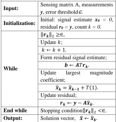
computational complexity than the optimization algorithms. The greedy methods that are commonly used in sparse signal recovery include the Matching Pursuit (MP) and its improvements. These improvements include the Orthogonal matching pursuit (OMP), Stagewise orthogonal matching pursuit (StOMP) and COmpressive Sampling Matching Pursuit (CoSaMP) algorithms [1][18]. The Matching Pursuit (MP) algorithm decomposes a signal into a linear expansion of elements that form a dictionary or sensing matrix A ∈ ℝM×N. At each successive iteration step of the algorithm, an element from the dictionary that best approximates the signal by reducing the residual is chosen. The algorithm can be described by the pseudo code given in table 1. The limitation of the MP algorithm is the lack of guarantees in terms of recovery error as well as the large number of iterations required.

The computational complexity drawback is

overcome by using the algorithm referred to as the Orthogonal Matching Pursuit (OMP) algorithm. The OMP method is a modification of the MP algorithm that bounds the maximum number of iterations

performed. The bounding gives a better

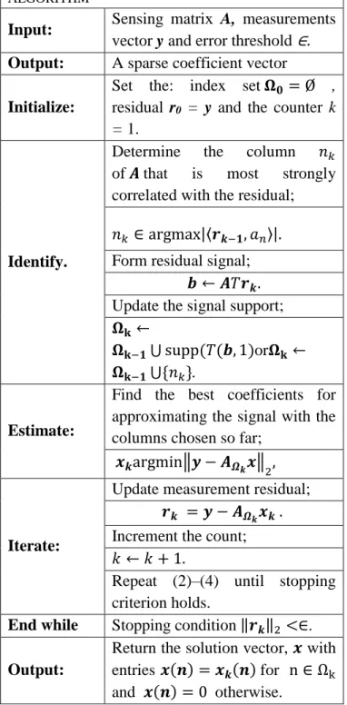
representation of the unexplained portion of the residual which is then subtracted from the current residual to form a new one. This process is iterated until a stopping condition is attained. Despite being fast as well as leading to exact sparse signal recovery, the guarantees associated with OMP are weaker than those achievable using optimization techniques. In spite of these drawbacks, the OMP algorithm is an efficient sparse signal recovery tool especially when the signal is highly sparse [19].The pseudo code of the OMP algorithm is as given in table 2. The reconstruction efficiency of the OMP algorithm is low when the signal is not highly sparse.

TABLE 1.THE MATCHING PURSUIT ALGORITHM

Input: Sensing matrix A, measurements

y, error threshold∈.

Initialization: Initial: signal estimate x0 = 0,

residual r0 = y, count k = 0.

While

‖𝒓𝒌‖2 ≥∈, Update 𝑘;

𝑘 ← 𝑘 + 1.

Form residual signal estimate;

𝒃 ← 𝑨𝑇𝒓_𝒌.

Update largest magnitude

coefficient;

𝒙

̂_𝒌 = 𝒙̂_𝒌−𝟏+ 𝑇(1).

Update residual;

𝒓_𝒌 ← 𝒚 − 𝑨𝒙̂_𝒌. End while Stopping condition‖𝒓_𝒌‖₂ <∈.

Output: Solution vector, 𝒙̂ ← 𝒙̂_𝒌.

The Stagewise Orthogonal Matching Pursuit (StOMP) method is an improvement of the OMP

algorithm that is characterized by lower

computational cost. The algorithm operates with a fixed number of stages during which it builds up a sequence of signal approximations by removing detected structures from a sequence of residuals [20]. The Compressive Sampling Matching Pursuit (CoSaMP) algorithm offers improvements to both the MP and OMP algorithms. The improvements are: reduction in computational complexity, stronger reconstruction guarantees as well as robustness to signal and measurement noise [4][18].

The IHT algorithm commences with an initial estimate of the target signal vector 𝒙̂. Next, iterative hard thresholding is applied to obtain a sequence of better signal estimates using the following iteration:

𝒙

(6)

Vol.2 No.2, 2018

TABLE 2.THE ORTHOGONAL MATCHING PURSUIT ALGORITHM

Input: Sensing matrix A, measurements

vector y and error threshold ∈.

Output: A sparse coefficient vector

Initialize:

Set the: index set 𝛀𝟎= Ø ,

residual r0 = y and the counter k

= 1.

Identify.

Determine the column 𝑛_𝑘

of 𝑨 that is most strongly

correlated with the residual;

𝑛_𝑘 ∈ argmax|〈𝒓_𝒌−𝟏, 𝑎_𝑛〉|.

Form residual signal;

𝒃 ← 𝑨𝑇𝒓_𝒌.

Update the signal support;

𝛀_𝐤 ←

𝛀_𝐤−𝟏⋃ supp(𝑇(𝒃, 1)or𝛀_𝐤 ← 𝛀𝐤−𝟏⋃{𝑛𝑘}.

Estimate:

Find the best coefficients for approximating the signal with the columns chosen so far;

𝒙_𝒌argmin‖𝒚 − 𝑨_𝜴_𝒌𝒙‖

2,

Iterate:

Update measurement residual;

𝒓_𝒌 = 𝒚 − 𝑨_𝜴_𝒌𝒙_𝒌 .

Increment the count;

𝑘 ← 𝑘 + 1.

Repeat (2)–(4) until stopping criterion holds.

End while Stopping condition ‖𝒓_𝒌‖₂ <∈.

Output:

Return the solution vector, 𝒙 with entries 𝒙(𝒏) = 𝒙𝒌(𝒏) for n ∈ Ωk and 𝒙(𝒏) = 0 otherwise.

The Bayesian CS reconstruction methods assume that the sparse signal comes from a known probability distribution. A stochastic measurements

vector y is used to recover the probability

distribution of each nonzero element of vector x. The recovery is done based on assumption of sparsity promoting priors. The method based on

Bayesian signal modeling approach does not have a well-defined reconstruction error guarantee [22].

B. Magnetic resonance imaging

Medical MRI is an imaging technique that utilizes the interaction between spinning hydrogen protons in the human body and an excitation RF signal. The interaction happens when the body is placed in a strong static magnetic field. The spinning protons precess about the longitudinal static magnetic field

𝑩_𝟎at the Larmor frequencyω₀ given by;

ω₀ = γ𝑩_𝟎, (13)

where γ is the gyromagnetic ratio of the hydrogen

protons whose value is given by γ 2𝜋⁄ = 42.57

MHz/T [8]. The interaction between 𝑩𝟎 and the spins give rise to a net magnetization moment 𝑴

that is related to 𝑩_𝟎 by;

𝑑𝑴

𝑑𝑡 = 𝑴 × γ𝑩𝟎. (14)

This net magnetization points in the direction (z) of

𝑩_𝟎 and has a magnitude M0 when the value of its

transverse component Mxy is zero. For an MR image

to be formed, the net magnetization needs to be flipped away from its equilibrium (z-direction) orientation. The magnetization also needs to be an oscillating function of time in order to produce induction of a current in the MRI equipment receiver coil [23].

Application of a transverse RF excitation signal pulse at the Larmor frequency induces a torque on the net magnetization causing it to flip away from its equilibrium axis. The tipping results in a non-zero

transverse component 𝑴_𝒙𝒚. The excitation RF pulse

is applied together with a slice-select gradient field

𝑮𝒛in order to excite only the slice of the patient’s body whose MR image is required [1][8]. Once the

excitation pulse is turned off, 𝑴_𝒙𝒚 decays

exponentially with a spin-spin relaxation time constant 𝑇2. At the same time, the longitudinal

component of the net magnetization 𝑴𝒛grows

(7)

Vol.2 No.2, 2018

field 𝑮_𝒚 and a frequency-encoding (read-out)

gradient field 𝑮_𝒚 respectively are applied before reading of the FID signal. The gradient fields add spatial information to the FID signal. The FID signal is a measure of 𝑴_𝒙𝒚which is given by the solution of following Bloch equation.

𝑑𝑴

𝑑𝑡 = 𝑴 × γ𝑩 − 𝑀𝑥

𝑇₂ 𝒂𝒙− 𝑀_𝑦

𝑇₂ 𝒂𝒚

−(𝑀𝑧− 𝑀0) 𝑇₁ 𝒂𝒛,

(15)

where 𝒂_𝒙, 𝒂_𝒚 and 𝒂_𝒛 are the unit vectors in the 𝑥, 𝑦

and 𝑧 directions respectively, 𝑴_𝒙(𝑡)a and 𝑴_𝒚(𝑡)

constitute the transverse magnetization component,

𝑩 is the effective magnetic field while 𝑴𝒛(𝑡) is the longitudinal component. The solution of the Bloch equation is;

𝑴(𝒓, 𝑡) =

𝑴_𝟎(𝒓)𝑒−𝑡 𝑇⁄ 2(𝒓)_𝑒−𝒋𝜔0𝑡_𝑒−𝑗2𝜋[𝑘𝑥(𝑡)𝑥 +𝑘𝑦(𝑡)𝑦]_, (16)

where 𝒓 = 𝑥𝒂_𝒙 + 𝑦𝒂_𝒚+ 𝑧𝒂_𝒛 is the Cartesian

position vector. The parameters 𝑘𝑥(𝑡) and 𝑘𝑦(𝑡) are the spatial frequency components given by;

𝑘_𝑥(𝑡) = 𝛾

2𝜋∫ 𝑮𝒙(𝜏)𝑑𝜏

𝒕

𝟎 and

𝑘𝑦(𝑡) = 𝛾

2𝜋∫ 𝑮𝒚(𝜏)𝑑𝜏 𝒕

𝟎 .

(17)

The receiver coil of the MRI equipment is designed to detect the transverse magnetization component contributions from all the precessing protons in the selected body slice. Therefore, the received FID signal 𝑠𝑟(𝑡) is proportional to the closed volume integral of the transverse magnetization as follows;

𝑠𝑟(𝑡) = ∭ 𝑴(𝒓, 𝑡)𝑑𝑥𝑑𝑦𝑑𝑧 (18)

Substituting for 𝑴(𝒓, 𝑡) from equation (16) in

equation (18) and assuming that 𝑇₂ ≫ 𝑡, the

demodulated FID signal is given by;

𝑠𝑟(𝑘𝑥, 𝑘𝑦)=

∭ 𝑴𝟎(𝒓)𝑒−𝑗2𝜋[𝑘𝑥(𝑡)𝑥 +𝑘𝑦(𝑡)𝑦]𝑑𝑥𝑑𝑦𝑑𝑧,

(19 )

Where 𝑠_𝑟(k_x, k_y) = 𝑠_𝑟(𝑡). When a thin zero-centered body slice (𝛥𝑧) is selectively excited, the demodulated FID signal will then be given by;

𝑠_𝑟(𝑘_𝑥, 𝑘_𝑦)

= ∬ 𝑴_𝒙𝒚𝑒−𝑗2𝜋[𝑘𝑥(𝑡)𝑥 +𝑘𝑦(𝑡)𝑦]_{𝑑𝑥𝑑𝑦,} (20)

where 𝑴_𝒙𝒚= ∫_{−𝛥𝑧 2}𝛥𝑧 2⁄_⁄ 𝑴_𝟎(𝒓)𝑑𝑧. The FID signal is therefore a two-dimensional Fourier transform of the

transverse magnetization 𝑴𝒙𝒚 at the spatial

frequency points ( 𝑘_𝑥, 𝑘_𝑦). In MRI, several FID signals are measured at different values of spatial frequencies. Each of these signals is sampled at the Nyquist rate in the spatial frequency domain at sampling periods of 𝛥𝑘𝑥 and 𝛥𝑘𝑦 to yield the

sampled signal 𝒮(u, v) such that;

𝒮(𝑢, 𝑣) = 𝑠_𝑟(𝑢𝛥_𝑘_𝑥, 𝑣𝛥_𝑘_𝑦) , (21)

where 𝑢 ∈ [(− (𝑁_𝑟⁄2)+ 1), 𝑁_𝑟⁄2], 𝑣 ∈

[(− (𝑁_𝑝⁄2)+ 1), 𝑁_𝑝⁄2], 𝑁_𝑟 is the number of read-out samples per acquisition and 𝑁_𝑝 is the number of phase encoding gradient steps.The sampled signals constitute the k-space of the MR image. The image is then reconstructed from the k-space using either the dimensional projection method or the two-dimensional Inverse Discrete Fourier transform (2D-IDFT) method.

The scan-time (𝑇𝑎) of conventional spin-echo MRI is related to the number of phase encoding steps(𝑁_𝑝) by;

𝑇𝑎 = (𝑇𝑅)(𝑁𝑝)(𝑁𝐸𝑋) , (22 )

Where 𝑇𝑅 is the pulse sequence repetition time and

𝑁𝐸𝑋 is the number of excitations used in the image

acquisition [1]. Therefore, if the parameters 𝑇𝑅 and

𝑁𝐸𝑋 are fixed, then, the image acquisition time is directly proportional to the number of phase encoding steps. The number of phase encoding steps required to satisfy the Nyquist sampling criterion is given by;

𝑁𝑝 ≈ 2(𝐹𝑜𝑉𝑦)( 𝑘𝑦𝑚𝑎𝑥), (23 )

where 𝐹𝑜𝑉𝑦 is the field of view of the image in the y- (phase encoding) direction while 𝑘_{𝑦𝑚𝑎𝑥} highest spatial frequency of the image in the y-direction. If the number of phase encoding steps used is lower

than 2(𝐹𝑜𝑉_𝑦)( 𝑘_{𝑦𝑚𝑎𝑥}) aliasing artifacts are

(8)

Vol.2 No.2, 2018

will be present in the reconstructed MR image. These artifacts manifest themselves in the image as the Gibb’s ringing phenomenon [1][8][23][24][25].

C). Objective image quality measures

Objective image metrics are used to compare the quality of a reconstructed image to that of its ground-truth version. The measures discussed in this section are the Mean Squared Error (MSE), the Peak Signal to Noise Ratio (PSNR) and the Structural SIMilarity (SSIM) index.

The MSE of a reconstructed image 𝒈 whose size

is 𝑃 × 𝑄 pixels is given by:

𝑀𝑆𝐸 =∑ ∑ [𝒇 − 𝐠]

2 𝑄

𝑦=1 𝑃

𝑥=1

𝑃𝑄𝐿2 ,

(24)

where 𝒇 is the 𝑃 × 𝑄 pixels ground-truth image and

𝐿 is the maximum pixel intensity of the ground-truth image. The PSNR of the reconstructed image is given by;

𝑃𝑆𝑁𝑅 = 10log10(

𝑃𝑄𝐿2 ∑ ∑𝑄 [𝒇 − 𝐠]2

𝑦=1 𝑃

𝑥=1

), (25)

Both the MSE and PSNR are simple to compute but they do not match well with the characteristics of the Human Visual System (HVS) [26].

The Structural SIMilarity (SSIM) index is a quantitative image quality metric that is based on

comparison of the luminance 𝑙(𝒇, 𝒈), contrast

𝑐(𝒇, 𝒈) and structure 𝑠(𝒇, 𝒈) factors of a reconstructed image with those of the ground-truth image. Unlike the MSE and PSNR measures, the SSIM index is consistent with the quality judgment of the HVS. The three components of the SSIM index are obtained from the means (𝜇), standard deviations (𝜎) as well as the cross-correlation (𝜎_𝑓𝑔)

between the images. The luminance comparison component is a function of the means of the images defined as:

𝑙(𝒇, 𝒈) = (2µ𝑓µ𝑔+ 𝐶1) (µ_𝑓2+ µ𝑔2 + 𝐶1)

, (26)

where µ𝑓and µ𝑔are the means of the images 𝒇 and

𝒈 respectively. The constant 𝐶₁ is assigned the value

𝐶₁ = [𝐾₁𝐿]2_where_𝐾

1 ≪ 1.The contrast component

is given by;

𝑐(𝒇, 𝒈) = (2𝜎𝑓𝜎𝑔+ 𝐶2) (𝜎_𝑓2+ 𝜎𝑔2+ 𝐶2)

, (27)

where 𝜎_𝑓 and 𝜎_𝑔 are the standard deviations of the images 𝒇 and 𝒈 respectively. The constant 𝐶₂ is assigned the value 𝐶2 = [𝐾2𝐿]2 where 𝐾2 ≪ 1. The structural component is a function of the standard deviations as well as the correlation between the images. It is given by;

𝑠(𝒇, 𝒈) = (𝜎𝑓𝑔+ 𝐶3)

(𝜎_𝑓𝜎_𝑔+ 𝐶₃), (28)

Where 𝜎𝑓𝑔 is the cross-correlation between the two images. The value of constant 𝐶₃ is 𝐶₃ = [𝐾₃𝐿]2

where 𝐾₃ ≪1. The SSIM index combines the three components as follows:

𝑆𝑆𝐼𝑀(𝒇, 𝒈) =

(𝑙(𝒇, 𝒈))α(𝑐(𝒇, 𝒈))β(𝑠(𝒇, 𝒈))γ, (29)

where 𝛼, 𝛽 and 𝛾 are parameters whose values are greater than zero and can be adjusted to alter the relative contributions of the three components. Substituting for the three components in equation (29) yields;

𝑆𝑆𝐼𝑀(𝒇, 𝒈) = ( (2µ𝑓µ𝑔 + 𝐶1) (µ_𝑓2 + µ_𝑔2 _{+ 𝐶}

1)

)

𝛼

×

( (2𝜎𝑓𝜎𝑔 + 𝐶2) (𝜎_𝑓2+ 𝜎𝑔2 + 𝐶2)

)

𝛽

((𝜎𝑓𝑔+ 𝐶3) (𝜎𝑓𝜎𝑔 + 𝐶3)

)

𝛾

(30)

Making the contributions of the three components to

be equal (𝛼 = 𝛽 = 𝛾 = 1) and setting 𝐶3 to

be 0.5𝐶2simplifies the SSIM index expression to;

𝑆𝑆𝐼𝑀(𝒇, 𝒈) =

(2µ_𝑓µ_𝑔 + 𝐶1) (2𝜎𝑓𝑔+ 𝐶2)

(µ_𝑓2₊_µ 𝑔

2 _{+ 𝐶}

1) (𝜎𝑓2+ 𝜎𝑔2+ 𝐶2)

. (31)

The SSIM index and its components satisfy the symmetry, boundedness and unique maximum properties [1][7][26].

III. PROPOSED METHOD AND DENOISING

(9)

Vol.2 No.2, 2018

mainly consists of three stages namely: selective

k-space sub-Nyquist acquisition, greedy CS

reconstruction and finally suppression of

concomitant artifacts. The method takes a shorter acquisition time (𝑇_𝑎) than conventional MRI since it uses only a fraction of the number of phase encoding gradient steps (𝑁𝑝) required to meet Nyquist sampling criterion.

A. The Proposed Algorithm

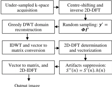
The entire proposed algorithm is illustrated in the block diagram given in fig. 1. The k-space under-sampling step involves the use of a few phase encoding gradient steps (𝑁_𝑝 < 2 (𝐹𝑜𝑣_𝑦)( 𝑘_{𝑦𝑚𝑎𝑥}) to selectively under-sample the k-space. The phase encoding steps used are chosen such that approximately half of the measurements are constituted by fully sampled rows at the center of the k-space. These rows contain the k-space

coefficients that have significantly larger

magnitudes than the coefficients in the outer k-space rows. The centered rows also correspond to low spatial frequencies. The remaining measurements are obtained by uniformly under-sampling the outer (high-frequency) k-space rows. The selective under-sampling process can be viewed as an elementwise matrix product of the full k-space of the image and an under-sampling mask as follows;

𝒮_𝑢(𝑢, 𝑣) = 𝒮(𝑢, 𝑣). ℳ(𝑢, 𝑣), (32) where 𝒮(𝑢, 𝑣) is the full k-space of the image,

𝒮𝑢(𝑢, 𝑣) is the under-sampled k-space and ℳ(𝑢, 𝑣) is the proposed under-sampling mask. The mask consist of all ones in the rows that correspond to the

rows of 𝒮(𝑢, 𝑣) that are to be included in

𝒮_𝑢(𝑢, 𝑣) and zeros in the remainder of its rows. For example, to selectively acquire 50% of the k-space of a 64 × 32 pixels image, only 32 out of the 64 rows of the k-space are captured. The central 16 rows of ℳ(𝑢, 𝑣) plus another 16 equally spaced rows selected from the remaining 48 outer (high frequency) rows will be filled with ones. Eight of the 16 high-frequency rows will be chosen from either side of the 16 central rows. The remaining 32 rows of ℳ(𝑢, 𝑣) are then filled with zeros. The

element-by-element product of ℳ(𝑢, 𝑣) and 𝒮(𝑢, 𝑣)

is equivalent to acquisition of an under-sampled version of the k-space using only half the number of

phase encoding steps dictated by the Nyquist sampling theorem. The acquired incomplete k-space is then transformed into an MR image by first centre-shifting it followed by determination of its Inverse 2D-DFT (2D-IDFT). The centre-shifting operation involves swapping of the first and fourth as well as second and third quadrants of the k-space matrix. This re-arrangement allows reconstruction of the image using MATLAB. The resulting image will be corrupted by coherent aliasing as well as Gibb’s ringing artifacts [1][11]. This noisy image is reshaped into a vector prior to fully sampling using a random sub-Gaussian matrix 𝜱 to yield a noisy measurement vector 𝒚′ given by;

𝒚′ _{= 𝜱𝒇}′_, ₍₃₃₎

where 𝒇′is the vectorized image. Next, the image is reconstructed from 𝒚′_{in form of vector}_𝒙_{in the} Haar DWT domain using the OMP greedy method in order to enforce the image sparsity. This step is followed by determination of the Inverse Discrete Wavelet Transform (IDWT) of vector 𝒙 to yield a second vectorized image signal 𝒇,, as follows;

𝒇,, _{= 𝚿}−𝟏_𝒙, ₍₃₄₎

where 𝚿−𝟏is the inverse of the Haar wavelet

transform matrix. The CS reconstruction of the image converts the coherent artifacts that are related

k-space under-sampling and truncation into

incoherent concomitant artifacts that are easily filtered [1]. The vectorized image 𝒇,,is then converted into its k-space data, 𝒮′(𝑢, 𝑣). This is achieved by first converting it into a matrix followed by determination of its centre-shifted 2D-DFT. In

𝒮′_{(𝑢, 𝑣)}_{, the k-space rows that were not captured} during the acquisition of 𝒮_𝑢(𝑢, 𝑣) will have been compressively reconstructed together with some artifacts. The k-space 𝒮′_{(𝑢, 𝑣)}_{is therefore a} corrupted version of full k-space of the MR image. This corrupted k-space is vectorized in order to simplify the design of a filter that suppresses the reconstruction artifacts. The vectorized k-space is multiplied by a proposed filter function as follows;

𝑆′′(𝑛) = 𝑆′_{(𝑛). ℎ(𝑛),} ₍₃₅₎

Where 𝑆′(𝑛) is the vectorized form of 𝒮′(𝑢, 𝑣),

𝑆′′(𝑛) is its filtered version while ℎ(𝑛) is the filter function. The range of the index 𝑛 for a 𝑃 × 𝑄

(10)

Vol.2 No.2, 2018

converted to the output image by first converting it into a matrix followed by inverse 2D-DFT determination.

In order to generate MATLAB simulation test results, an MR image is first converted into its k-space by obtaining its centre-shifted 2D-DFT. The k-space data is then processed according to the procedure illustrated in fig. 1.

B. The proposed filter function

The proposed artifacts suppression filter

accentuates the high frequency k-space coefficients by a scaling correction factor 𝜌 > 1 without affecting the low frequency coefficients. The filter characteristic was suggested after observing that the CS reconstruction resulted in a reduction in the magnitudes of high frequency k-space coefficient with negligible effects on the low frequency ones.

The filter function h(n) is given by;

ℎ(𝑛) = {1 𝑓𝑜𝑟 𝑁1 ≤ 𝑛 ≤ 𝑁2

𝜌 elsewhere , (36)

where 𝜌 is the correction factor while 𝑁₁ and 𝑁₂ are the indexes of the vectorized k-space that define the range of the fully sampled low frequency k-space coefficients.

Figure 1. The proposed algorithm block diagram.

IV. EXPERIMENTAL RESULTS

For the purpose of demonstrating the

effectiveness of the proposed algorithm, MATLAB simulation results of ten MR images were obtained.

The MR images were first down-sized to 64 × 32

pixels using bicubic interpolation in order to reduce the processing time. The resizing also enabled the use of a denoising filter that does not require many parameters adjustments. The images were obtained from various sources that include the Siemens Healthineers [27] and the MNI BITE [28] databases. Results of some specific images as well as statistical summaries of the reconstruction qualities for all the images are presented. In all the experiments, the value of the artifacts correction factors used was in the range of 1.0 ≤ 𝜌 ≤ 1.4. An artifacts correction factor of 𝜌 = 1.2 was found to consistently give reconstruction results of the highest quality.

A. The proposed algorithm illustrations

Figure 2 shows an illustration of the selective k-space under-sampled acquisition and reconstruction of the denoised image stages of the proposed method. At the top of column (a) is the ground-truth image which is a sagittal cross-section of a head MR image. Its full k-space is given below it in the same column. Part (b) presents an under-sampled image that is reconstructed from 50 % of the full k-space rows as shown in the same column below the image. The under-sampled image is corrupted by coherent aliasing as well as truncation artifacts. Column (c) shows the image reconstructed using the proposed methods plus its k-space. It is evident from column (c) that most of the coefficients missing in the k-space given in part (b) have been compressively recovered. These results demonstrate that it is possible to approximately reconstruct the MR image from its under-sampled k-space.

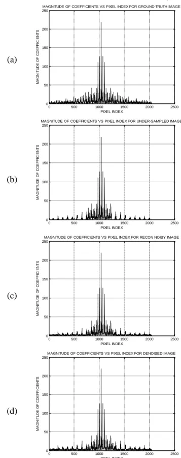
The results presented in fig. 3 demonstrate the effect of the artifacts suppression filter on the magnitude of the k-space coefficients. In all the plots, the zero spatial frequency coefficient is located at the centre and has a magnitude of 872.64. This coefficient has been scaled down by a factor of four to 218.16 in order to make it possible for the higher frequency coefficients located further from the centre to be seen more clearly.

Centre-shifting and inverse 2D-DFT Under-sampled k-space

acquisition

Random sampling: 𝒚′₌ 𝜱𝒇′

2D-DFT determination and vectorization IDWT and vector to

matrix conversion

Artifacts suppression:

𝑆′′_(𝑛)₌_𝑆′_{(𝑛). ℎ(𝑛)}

Vector to matrix, and 2D-IDFT Greedy DWT domain

reconstruction

(11)

Vol.2 No.2, 2018

(a) (b) (c)

Figure 2. Illustration of the proposed method. (a) Ground-truth head MR image and its k-space. (b) Selectively under-sampled image and its k-space. (c) Denoised output image and its k-space.

Part (a) presents a plot of the magnitudes of the k-space coefficients of a ground-truth head MR image versus the pixel index. The k-space has been vectorized in order to simplify the design of the artifacts suppression filter. The under-sampled version of the k-space of the image using 50% of the phase encoding steps is shown in part (b). In part (c), the vectorized k-space that has been compressively reconstructed from the under-sampled version in part (b) is presented prior to denoising. It is evident that the coefficients missing in part (b) have been reconstructed in part (c). However, some of the reconstructed high-frequency coefficients have magnitudes that are much lower than their corresponding coefficients in part (a). Part (d) shows the reconstructed k-space of the image after denoising. The parameters of the denoising filter used: ρ = 1.2, 𝑁₁ = 768 and 𝑁₂ = 1280.

Comparing parts (d) and (c), the filter has the effect of increasing the magnitudes of the high frequency k-space coefficients to be comparable to those of the ground-truth image without affecting the low frequency coefficients.

(a)

(b)

(c)

(d)

Figure 3. Denoising effect on vectorized k-space.(a) Ground-truth k-space. (b) Under-sampled k-space. (c) The reconstructed k-space. (d) Denoised k-space.

0 500 1000 1500 2000 2500

0 50 100 150 200 250

MAGNITUDE OF COEFFICIENTS VS PIXEL INDEX FOR GROUND-TRUTH IMAGE

M A G N IT U D E O F C O E F F IC IE N T S PIXEL INDEX

0 500 1000 1500 2000 2500

0 50 100 150 200 250

MAGNITUDE OF COEFFICIENTS VS PIXEL INDEX FOR UNDER-SAMPLED IMAGE

0 500 1000 1500 2000 2500

0 50 100 150 200 250

MAGNITUDE OF COEFFICIENTS VS PIXEL INDEX FOR RECON NOISY IMAGE

0 500 1000 1500 2000 2500

0 50 100 150 200 250

MAGNITUDE OF COEFFICIENTS VS PIXEL INDEX FOR DENOISED IMAGE

(12)

Vol.2 No.2, 2018

B. Reconstruction quality comparison

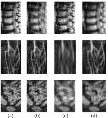
In fig.4, the reconstruction results for three MR images (spine, leg, and intestines) using three different methods at 40% measurements are shown. Column (a) presents the ground-truth images. The images reconstructed using the OMP and StOMP greedy algorithms are shown in columns (b)and (c) respectively. The images reconstructed using the proposed method are presented in column (d). These results show that, the proposed method gives higher quality of reconstruction compared to the other two methods.

The reconstruction quality assessment results for three MR images (knee, spine hand) reconstructed using different CS-MRI methods are presented in table 3. The reconstructions were performed at different percentage measurements using the proposed method as well as the OMP and StOMP methods. The left-most column shows the three MR images while the next one lists the percentages of the k-space rows that were selectively acquired.

(a) (b) (c) (d)

Figure 4.Image reconstruction results. (a) Input ground-truth MR images. (b) Reconstruction using the OMP method. (c) Reconstruction using the StOMP method. (d) Reconstruction using the proposed method.

TABLE 3. THE SSIM VALUES OF RECONSTRUCTED IMAGES

MR Image %Measur -ements

OMP StOMP Proposed SSIM SSIM SSIM 10 0.56 0.54 0.74 20 0.77 0.75 0.85 30 0.86 0.78 0.90 40 0.90 0.82 0.94 50 0.93 0.90 0.96 60 0.95 0.93 0.98 70 0.96 0.94 0.99 10 0.63 0.62 0.76 20 0.77 0.76 0.86 30 0.83 0.80 0.94 40 0.89 0.88 0.95 50 0.93 0.90 0.96 60 0.95 0.93 0.97 70 0.97 0.95 0.98 10 0.81 0.73 0.88 20 0.91 0.89 0.93 30 0.95 0.93 0.95 40 0.96 0.96 0.97 50 0.98 0.97 0.98 60 0.98 0.98 0.98 70 0.98 0.98 1.00

(13)

Vol.2 No.2, 2018

TABLE 4. THE PSNR VALUES OF RECONSTRUCTED IMAGES

MR Image % Measure ments

OMP StOMP Proposed PSNR

(dB)

PSNR (dB)

PSNR (dB) 10 13.07 14.13 17.24 20 14.66 15.78 19.01 30 16.54 16.43 21.43 40 18.16 17.41 22.96 50 19.07 18.35 24.48 60 20.85 19.68 25.14 70 22.97 20.94 27.05 10 14.91 15.59 19.56 20 16.07 16.68 20.60 30 17.44 18.09 22.75 40 18.70 18.80 24.05 50 20.61 19.59 26.13 60 21.95 20.36 27.78 70 23.52 22.07 29.01 10 15.31 16.58 18.38 20 18.15 18.70 20.13 30 18.63 19.55 22.37 40 20.40 20.69 23.40 50 21.63 21.12 24.88 60 22.59 21.98 25.13 70 24.43 23.07 26.45 70 26.25 24.05 27.25

C. Statistical summary

A statistical mean of the quality for all the ten MR images reconstructed using the proposed method as well the OMP and StOMP methods is graphically presented in fig. 5. The mean PSNR values of the reconstructed images are plotted for different percentage measurements. The proposed method yielded higher quality images than the other two methods in terms of the PSNR measure. The quality improvement is at least 1.75 dB for 20% or more measurements. From the graphs, the OMP and StOMP methods would require at least 20% more measurements to reconstruct images of the same quality as those of the proposed method. For example, to reconstruct an image whose PSNR is 21.4 dB, the OMP method requires 50% of the full k-space. On the other hand, the proposed method requires only 30% of the full k-space coefficients to reconstruct an image whose PSNR is 21.6 dB. This 20% reduction in the percentage measurements required by the proposed method for a given reconstruction quality is equivalent to a 20% reduction in the phase encoding gradient steps (𝑁_𝑝)

required. From equation (22), a 20% reduction in 𝑁_𝑝

for a given image quality is equivalent to a 20% reduction in the MRI scan time.

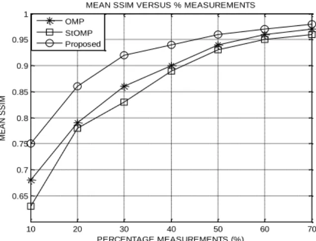
Almost similar results to the mean PSNR results presented in fig. 5 were obtained using the SSIM quality measure as shown in fig. 6. The figure presents a plot of the mean SSIM values of the reconstructed images at different percentage measurements for the OMP, StOMP and proposed methods. The mean SSIM values of the proposed method are consistently higher than for the other two methods. From the graphs, the OMP and StOMP methods would require about 20% more measurements to reconstruct images of the same quality as those of the proposed method. The images reconstructed using the StOMP method at 50% measurements have a mean SSIM index of 0.93. However, the proposed method requires only 30% measurements to reconstruct images whose mean SSIM index is 0.92 dB.

Figure 5. Statistical mean of PSNR for different reconstruction methods.

Figure 6. Statistical mean of SSIM for OMP, StOMP and proposed methods.

10 20 30 40 50 60 70 14

16 18 20 22 24 26 28

MEAN PSNR VERSUS PERCENTAGE MEASUREMENTS

PERCENTAGE MEASUREMENTS (%)

M

E

A

N

P

S

N

R

OMP StOMP Proposed

10 20 30 40 50 60 70

0.65 0.7 0.75 0.8 0.85 0.9 0.95 1

MEAN SSIM VERSUS % MEASUREMENTS

M

E

A

N

S

IM

(14)

Vol.2 No.2, 2018

Figure 7 presents the variation of the variance of the PSNR measures of the images reconstructed using three different methods at different percentage measurements. On average, the proposed method yields lower variance values than both the OMP and StOMP methods. The lower values of variance confirm that the proposed method exhibits better consistency in reconstruction quality than the other two methods.

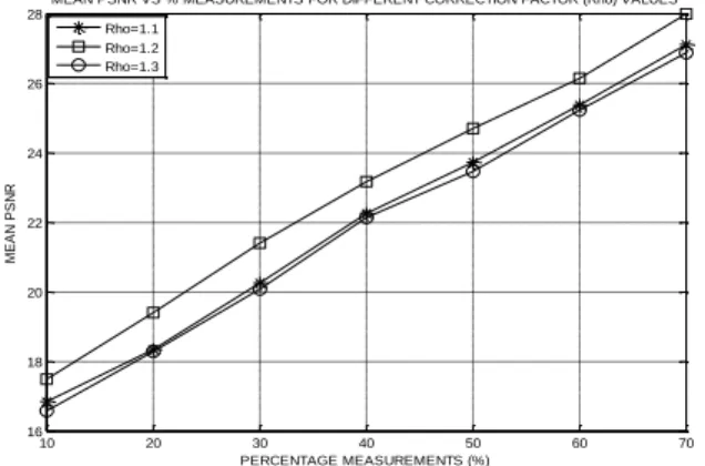
The variation in performance of the proposed

method with the correction factor (𝜌) of the

proposed filter function is presented in fig. 8. These

results show that a correction factor of

approximately 1.2 yields optimum quality results in terms of the PSNR for all the measurements tested. Using the SSIM index, similar results were obtained and approximately the same optimum value of the correction factor was obtained. The quality of the reconstructed images was found to decrease monotonically as the value of the correction factor

used deviates from the optimum value of 𝜌 = 1.2.

Figure 7. Variation of the variance of PSNR for different reconstruction methods.

Figure 8. Performance variation of the proposed method with the correction factor.

V. CONCLUSION

A fast and robust method for reconstruction of MR images has been proposed in this paper. The method utilizes sparse reconstruction of sub-Nyquist sampled k-space data of the image in the DWT domain. An apodizing filter function has also been used to enhance the rubustness of the method. Computer simulation reconstruction results of the proposed method have been used to demonstrate a quality improvement of at least 1.75 dB and up to 2.1 dB over the OMP method when using at least 20% of the full k-space data. For a given desired reconstruction quality and while using at least 30% measurements, the proposed method requires 20% fewer measurements than both the OMP and StOMP methods. This reduction in the phase encoding steps requirement implies a 20% reduction in the image acquisition time. This research will be pursued further with an aim of further reducing both the artifacts in the reconstructed images and the scan-time. To achieve the improvements, variable density under-sampling approaches as well as different artifacts filter functions will be tested.

REFERENCES

[1] H. Kiragu, E. Mwangi, and G. Kamucha, “A

Rapid MRI Reconstruction Method Based on

Compressive Sampling and Concomitant

Artifacts Suppression,” Proceedings on IEEE

MELECON 2018 conference, Marrakech,

Morocco, May 2018.

[2] E. J. Candes and M. B. Wakin, “Introduction to

compressive sampling: a sensing/sampling paradigm that goes against the common knowledge in data acquisition,” IEEE Signal Processing Magazine, March 2008, pp. 21-30.

[3] S. Foucart and H. Rauhut, A mathematical

introduction to compressive sensing, 1st edition, Springer Science and Business Media, 2013.

[4] C. E. Yonina and G. Kutyniok, Compressed

sensing theory and applications, 1st edition, Cambridge University Press, 2015.

[5] J. Qianru, C. Rodrigo, L. Sheng, and B. Huang,

“Joint sensing matrix and sparsifying dictionary

optimization applied in real image for

compressed sensing,” Proceedings on

International Digital Signal Processing , London, United Kingdom, August 2017.

10 20 30 40 50 60 70

0.5 1 1.5 2 2.5 3 3.5 4 4.5 5 5.5

VARIANCE OF THE PSNR VERSUS % MEASUREMENTS

V

A

R

IA

N

C

E

O

F

T

H

E

P

S

N

R

OMP StOMP Proposed

10 20 30 40 50 60 70

16 18 20 22 24 26 28

MEAN PSNR VS % MEASUREMENTS FOR DIFFERENT CORRECTION FACTOR (Rho) VALUES

M

E

A

N

P

S

N

R

(15)

Vol.2 No.2, 2018

[6] R. G. Baraniuk, V. Cevher, M. Duarte, and C. Hedge, “Model-based compressive sensing,” IEEE Transaction on Information Theory, 2010, vol. 56 (4), pp. 1982-2001.

[7] H. Kiragu, E. Mwangi, and G. Kamucha, “A

hybrid MRI method based on denoised compressive sampling and detection of dominant

coefficients,” proceedings onInternational

Digital Signal Processing, London, United Kingdom, August 2017.

[8] R. H. Hashemi, W. G. Bradley, and C. J. Lisanti,

MRI the Basics, 3rd edition, Philadelphia, USA: Lippincott Williams & Wilkins, 2010.

[9] M. Lustig, Sparse MRI, PhD thesis, Stanford University, California, USA, 2008.

[10]M. Vlaardingerbroek, J.A. den Boer, Magnetic

resonance imaging, 2nd edition, Springer, 1999.

[11]S. S.Vasanawala, M. Alley, R. Barth, B.

Hargreaves, J. Pauly, and M. Lustig, “Faster pediatric MRI via compressed sensing,” proceedings on annual meeting of the Society of Ped. Rad. (SPR), Carlsbad, CA, April 2009. [12]T. Kustner, C. Wurslin, S. Gatidis et al., “MR

image reconstruction using a combination of

compressed sensing and partial Fourier

acquisition: ESPReSSo,” IEEE Transactions on Medical Imaging, 2016, vol. 35 (11), pp. 2447-2458.

[13]R. K. Nandini, Compressive sensing based

image processing and energy-efficient hardware implementation with application to MRI and JPEG 2000, PhD dissertation, University of Southern Queensland, Australia, 2014.

[14]J. Vellagoundar and M. R. Reddy “Optimal k-space sampling scheme for CS-MRI,” IEEE EMBS International Conference on Biomed. Eng. and Sciences, Langkawi, Malaysia, Dec. 2012.

[15]H. Kiragu, E. Mwangi, and G. Kamucha, “A

robust magnetic resonance imaging method based on compressive sampling and clustering of sparsifying coefficients,” proceedings of IEEE MELECON 2016 conference, Limassol, Cyprus April 2016.

[16]Z. Zangen, W. Khan, B. Paul, and Y. Ran,

“Compressed sensing based MRI

reconstruction using complex double-density

dual-tree DWT,” International Journal of Biomedical Imaging, 2013.

[17]L. Chun-Shien and C. Hung-Wei, “Compressive

image sensing for fast recovery from limited samples: A variation on compressive sensing,” Elsevier journal of Information Sciences, vol. 325, pp. 33–47, 2015.

[18]D. Needell and J. Tropp. COSaMP: Iterative

signal recovery from incomplete and inaccurate samples. Appl. Comput. Harmon. Anal., 26 (3): 3018211; 321, 2009.

[19]J. Tropp and A. Gilbert. Signal recovery from partial information via orthogonal matching pursuit. IEEE Trans. Inform. Theory, 53 (12): 46558211; 4666, 2007.

[20]D. Donoho, I. Drori, Y. Tsaig, and J. L. Stark. “Sparse solution of under determined linear equations by stagewise orthogonal matching pursuit,” Tech report, Stanford University, 2006.

[21]T. Blumensath and M. E. Davies, “Iterative

hard thresholding for compressed sensing,” Applied and Computational Harmonic Analysis, vol. 27, no. 3, pp. 265–274, 2009.

[22]S. Sarvotham, D. Baron, and R. Baraniuk.

Compressed sensing reconstruction via belief propagation. Technical report TREE-0601, Rice University, Texas, USA, 2006.

[23]R. W. Brown, Y. N. Cheng, E. M. Haacke, M. R. Thompson, and R. Venkatesan, Magnetic Resonance Imaging: Physical Principles and Sequence Design, 2nd edition, John Wiley & Sons, 2014.

[24]M. A. Bernstein, K. F. King and X. J. Zhou, Handbook of MRI Pulse Sequences, Elsevier Academic Press, 2004.

[25]D. G. Nishimura, Principles of Magnetic

Resonance Imaging, Stanford University, 1996.

[26]Z. Wang and C. Bovik, “A universal image

quality index,” IEEE Signal Processing Letters, 2002, vol. 9 (3), pp. 81–84.

[27]Siemens Healthineers. “Dicom Images.”

internet https://www. healthcare. siemens.com/ magnetic-resonance-imaging/ magnetom-world/ clinical-corner/ protocols/dicom-images, [Dec. 16, 2017].

[28]The MNI BITE, internet, http://www.bic.mni.