arXiv:1708.00072v1 [cs.LO] 31 Jul 2017
A Component-oriented Framework for Autonomous Agents
Tobias Kappé
∗1, Farhad Arbab
2,3, and Carolyn Talcott
4 1University College London, London, United Kingdom
2Centrum Wiskunde & Informatica, Amsterdam, The Netherlands
3
LIACS, Leiden University, Leiden, The Netherlands
4SRI International, Menlo Park, USA
Abstract
The design of a complex system warrants a compositional methodology, i.e., composing simple components to obtain a larger system that exhibits their collective behavior in a mean-ingful way. We propose an automaton-based paradigm for compositional design of such systems where an action is accompanied by one or more preferences. At run-time, these preferences provide a natural fallback mechanism for the component, while at design-time they can be used to reason about the behavior of the component in an uncertain physical world. Using structures that tell us how to compose preferences and actions, we can compose formal rep-resentations of individual components or agents to obtain a representation of the composed system. We extend Linear Temporal Logic with two unary connectives that reflect the compo-sitional structure of the actions, and show how it can be used to diagnose undesired behavior by tracing the falsification of a specification back to one or more culpable components.
1
Introduction
Consider the design of a software package that steers a crop surveillance drone. Such a system (in its simplest form, a single drone agent) should survey a field and relay the locations of possible signs of disease to its owner. There are a number of concerns at play here, including but not limited to maintaining an acceptable altitude, keeping an eye on battery levels and avoiding birds of prey. In such a situation, it is best practice to isolate these separate concerns into different modules — thus allowing for code reuse, and requiring the use of well-defined protocols in case coordination between modules is necessary. One would also like to verify that the designed system satisfies desired properties, such as “even on a conservative energy budget, the drone can always reach the charging station”.
In the event that the designed system violates its verification requirements or exhibits behavior that does not conform to the specification, it is often useful to have an example of such behavior. For instance, if the surveillance drone fails to maintain its target altitude, an example of behav-ior where this happens could tell us that the drone attempted to reach the far side of the field and ran out of energy. Additionally, failure to verify an LTL-like formula typically comes with a counterexample — indeed, a counterexample arises from the automata-theoretic verification ap-proach quite naturally [33]. Taking this idea ofdiagnostics one step further in the context of a compositional design, it would also be useful to be able to identify the components responsible for allowing a behavior that deviates from the specification, whether this behavior comes from a run-time observation or a design-time counterexample to a desired property. The designer then knows which components should be adjusted (in our example, this may turn out to be the route planning component), or, at the very least, rule out components that are not directly responsible (such as the wildlife evasion component).
In this paper, we propose an automata-based paradigm based on Soft Constraint Automata [1, 20], called Soft Component Automata (SCAs1). An SCA is a state-transition system where tran-sitions are labeled with actions and preferences. Higher-preference trantran-sitions typically contribute more towards the goal of the component; if a component is in a state where it wants the system to move north, a transition with actionnorth has a higher preference than a transition with ac-tionsouth. At run-time, preferences provide a natural fallback mechanism for an agent: in ideal circumstances, the agent would perform only actions with the highest preferences, but if the most-preferred actions fail, the agent may be permitted to choose a transition of lower preference. At design-time, preferences can be used to reason about the behavior of the SCA in suboptimal condi-tions, by allowing all actions whose preference is bounded from below by a threshold. In particular, this is useful if the designer wants to determine the circumstances (i.e., threshold on preferences) where a property is no longer verified by the system.
Because the actions and preferences of an SCA reside in well-defined mathematical structures, we can define a composition operator on SCAs that takes into account the composition of actions as well as preferences. The result of composition of two SCAs is another SCA where actions and preferences reflect those of the operands. As we shall see, SCAs are amenable to verification against formulas in Linear Temporal Logic (LTL). More specifically, one can check whether the behavior of an SCA is contained in the behavior allowed by a formula of LTL.
Soft Component Automata are a generalization of Constraint Automata [3]. The latter can be used to coordinate interaction between components in a verifiable fashion [2]. Just like Constraint Automata, the framework we present blurs the line betweencomputationandcoordination— both are captured by the same type of automata. Consequently, this approach allows us to reason about these concepts in a uniform fashion: coordination is not separate in the model, it is effected by components which are inherently part of the model.
We present two contributions in this paper. First, we propose an compositional automata-based design paradigm for autonomous agents that contains enough information about actions to make agents behave in a robust manner — by which we mean that, in less-than-ideal circumstances, the agent has alternative actions available when its most desired action turns out to be impossible, which help it achieve some subset of goals or its original goals to a lesser degree. We also put forth a dialect of LTL that accounts for the compositional structure of actions and can be used to verify guarantees about the behavior of components, as well as their behavior in composition. Our second contribution is a method to trace errant behavior back to one or more components, exploiting the algebraic structure of preferences. This method can be used with both run-time and design-time failures: in the former case, the behavior arises from the action history of the automaton, in the latter case it is a counterexample obtained from verification.
In Section 2, we mention some work related to this paper; in Section 3 we discuss the necessary notation and mathematical structures. In Section 4, we introduce Soft Component Automata, along with a toy model. We discuss the syntax and semantics of the LTL-like logic used to verify properties of SCAs in Section 5. In Section 6, we propose a method to extract which components bear direct responsibility for a failure. Our conclusions comprise Section 7, and some directions for further work appear in Section 8.
Acknowledgements The authors would like to thank Vivek Nigam and the anonymous FACS-referees for their valuable feedback. This work was partially supported by ONR grant N00014–15– 1–2202.
2
Related Work
The algebraic structure for preferences called theConstraint Semiringwas proposed by Bistarelli et al. [5, 4]. Further exploration of the compositionality of such structures appears in [12, 15, 20]. The structure we propose for modeling actions and their compositions is an algebraic reconsideration ofstatic constructs[16].
1
The automata formalism used in this paper generalizesSoft Constraint Automata[3, 1]. The latter were originally proposed to give descriptions of Web Services [1]; in [20], they were used to model fault-tolerant, compositional autonomous agents. Using preference values to specify the behavior of autonomous agents is also explored from the perspective of rewriting logic in theSoft Agent Framework[31, 32]. Recent experiments with the Soft Agent Framework show that behavior
based on soft constraints can indeed contribute robustness [22].
Sampath et al. [28] discuss methods to detect unobservable errors based on a model of the system and a trace of observable events; others extended this approach [11, 25] to a multi-component setting. Casanova et al. [9] wrote about fault localisation in a system where some components are inobservable, based on which computations (tasks involving multiple components) fail. In these paradigms, one tries to find out where aruntime fault occurs; in contrast, we try to find out which component is responsible forundesired behavior, i.e., behavior that is allowed by the system but not desired by the specification.
A general framework for fault ascription in concurrent systems based on counterfactuals is presented in [13, 14]. Formal definitions are given for failures in a given set of components to be necessary and/or sufficient cause of a system violating a given property. Components are specified by sets of sets of events (analogous to actions) representing possible correct behaviors. A parallel (asynchronous) composition operation is defined on components, but there is no notion of composition of events or explicit interaction between components. A system is given by a global behavior (a set of event sets) together with a set of system component specifications. The global behavior, which must be provided separately, includes component events, but may also have other events, and may violate component specifications (hence the faulty components). In our approach, global behavior is obtained by component composition. Undesired behavior may be local to a component or emerge as the result of interactions.
In LTL, a counterexample to a negative result arises naturally if one employs automata-based verification techniques [24, 33]. In this paper, we further exploit counterexamples to gain informa-tion about the component or components involved in violating the specificainforma-tion. The applicainforma-tion of LTL to Constraint Automata is inspired by an earlier use of LTL for Constraint Automata [2].
Some material in this paper appeared in the first author’s master’s thesis [18].
3
Preliminaries
If Σ is a set, then 2Σdenotes the set of subsets of Σ, i.e., thepowerset of Σ. We write Σ∗ for the
set offinite words over Σ, and if σ∈Σ∗ we write|σ| for the length of σ. We writeσ(n) for the
n-th letter ofσ(starting at 0). Furthermore, let Σωdenote the set of functions fromNto Σ, also
known as streamsover Σ [26]. We define for σ ∈Σω that |σ| =ω (the smallest infinite ordinal).
Concatenation of a stream to a finite word is defined as expected. We use the superscriptω to denote infinite repetition, writingσ =h0,1iω for the parity function; we write Σπ for the set of
eventually periodic streams in Σω, i.e.,σ∈Σωsuch that there exist σ
h, σt∈Σ∗ withσ=σh·σωt.
We writeσ(k) withk∈Nfor thek-th derivative ofσ, which is given byσ(k)(n) =σ(k+n). IfS is a set and ⊙:S×S→S a function, we refer to⊙as anoperator onS and writep⊙q
instead of⊙(p, q). We always use parentheses to disambiguate expressions if necessary. To model composition of actions, we need a slight generalization. IfR⊆S×S is a relation and⊙:R→S
is a function, we refer to⊙as apartial operator onS up toR; we also use infix notation by writing
p⊙qinstead of⊙(p, q) wheneverpRq. If ⊙:R→S is a partial operator onS up toR, we refer to ⊙as idempotent if p⊙p=p for allp∈ S such thatpRp, and commutative ifp⊙q =q⊙p
wheneverp, q∈S,pRq andqRp. Lastly,⊙isassociative if for all p, q, r∈S, pRqand (p⊙q)Rr
if and only ifqRr and pR(q⊙r), either of which implies that (p⊙q)⊙r =p⊙(q⊙r). When
R=S×S, we recover the canonical definitions of idempotency, commutativity and associativity. Aconstraint semiring, orc-semiring, provides a structure on preference values that allows us to
compare the preferences of two actions to see if one is preferred over the other as well ascompose
preference values of component actions to find out the preference of their composed action. A c-semiring [5, 4] is a tuplehE,L
,⊗,0,1isuch that (1)Eis a set, called thecarrier, with0,1∈E, (2)L : 2E
→ Eis a function such that for e ∈E we have that L∅ =0and LE =1, as well as L{
e} =e, and for E ⊆ 2E
, also L{L(
(3) ⊗: E×E → E is a commutative and associative operator, such that fore ∈E and E ⊆E, it holds that e⊗0= 0and e⊗1 =e as well as e⊗L
E =L{
e⊗e′ : e′ ∈E}. We denote a c-semiring by its carrier; if we refer toEas a c-semiring, associated symbols are denotedL
E,0E, et cetera. We drop the subscript when only one c-semiring is in context.
The operatorLof a c-semiringEinduces an idempotent, commutative and associative binary operator⊕: E×E→ E by defining e⊕e′ =L({
e, e′}) The relation ≤E ⊆E×E is such that
e≤Ee′ if and only ife⊕e′=e′;≤Eis a partial order onE, with0and1the minimal and maximal elements [4]. All c-semirings are complete lattices, withL
filling the role of the least upper bound operator [4]. Furthermore,⊗is intensive, meaning that for anye, e′ ∈E, we have e⊗e′ ≤e[4].
Lastly, when⊗is idempotent,⊗coincides with the greatest lower bound [4]. Models of a c-semiring includeW=R≥0∪ {∞},inf,+ˆ,∞,0
(the weighted semiring), where inf is the infimum and ˆ+ is arithmetic addition generalized toR≥0∪ {∞}. Here,≤Wcoincides with the obvious definition of the order≥onR≥0∪ {∞}. Composition operators for c-semirings exist, such as product composition [6] and (partial) lexicographic composition [12]. We refer to [20] for a self-contained discussion of these composition techniques.
4
Component Model
We now discuss our component model for the construction of autonomous agents.
4.1
Component Action Systems
Observable behavior of agents is the result of the actions put forth by their individual components; we thus need a way to talk about how actions compose. For example, in our crop surveillance drone, the following may occur:
• The component responsible for taking pictures wants to take a snapshot, while the routing component wants to move north. Assuming the camera is capable of taking pictures while moving, these actions may compose into the action “take a snapshot while moving north”. In this case, actions compose concurrently, and we say that the latter action captures the former two.
• The drone has a single antenna that can be used for GPS and communications, but not both at the same time. The component responsible for relaying pictures has finished its transmission and wants to release its lock on the antenna, while the navigation component wants to get a fix on the location and requests use of the antenna. In this case, the actions “release privilege” and “obtain privilege” composelogically, into a “transfer privilege” action.
• The routing component wants to move north, while the wildlife avoidance component notices a hawk approaching from that same direction, and thus wants to move south. In this case, the intentions of the two components are contradictory; these component actions are incom-posable, and some resolution mechanism (e.g., priority) will have to decide which action takes precedence.
All of these possibilities are captured in the definition below.
Definition 1. A Component Action System (CAS) is a tuple hΣ,⊚,i, such that Σ is a finite set ofactions,⊚⊆Σ×Σ is a reflexive and symmetric relation and:⊚→Σ is an idempotent, commutative and associative operator on Σ up to⊚(i.e.,is an operator defined only on elements of Σ related by⊚). We call⊚thecomposability relation, andthecomposition operator.
Every CAShΣ,⊚,iinduces a relation ⊑on Σ, where fora, b∈Σ, a⊑b if and only if there exists ac∈Σ such thataandcare composable (a⊚c) and they compose intob (ac=b). One can easily verify that⊑is a preorder; accordingly, we call⊑thecapture preorder of the CAS.
We model incomposability of actions by omitting them from the composability relation; i.e., if
southis an action that compels the agent to move south, whilenorthdrives the agent north, we set
south6⊚north. Note that⊚is not necessarily transitive. This makes sense in the scenarios above, where snapshot is composable with south as well as north, but north is incomposable with south. Moreover, incomposability carries over to compositions: ifsouth⊚snapshotandsouth6⊚north, also (southsnapshot)6⊚north. This is formalized in the following lemma.
Lemma 1. Let hΣ,⊚,i be a CAS and let a, b, c ∈ Σ. If a⊚b but a 6⊚ c, then (ab) 6⊚ c.
Moreover, if a6⊚c anda⊑b, thenb6⊚c.
Proof. For the first claim, suppose that (ab)⊚c. Then, since is associative up to ⊚, it follows thatb⊚canda⊚(bc), which contradicts the premise thatb6⊚c. We thus conclude that (ab)6⊚c.
For the second claim, suppose thata6⊚c anda⊑b. Then there exists ad∈Σ such thata⊚d
andad=b. By the above,b= (ad)6⊚c.
The composition operator facilitates concurrent as well as logical composition. Given actions
obtain,releaseandtransfer, with their interpretation as in the second scenario, we can encode that
obtainandreleaseare composable by stipulating that obtain⊚release, and say that their (logical) composition involves an exchange of privileges by choosingobtainrelease=transfer. Furthermore, the capture preorder describes our intuition of capturing: ifsnapshotandmoveare the actions of the first scenario, withsnapshot⊚north, thensnapshot,north⊑snapshotnorth.
Port Automata [21] contain a model of a CAS. Here, actions are sets of symbols calledports, i.e., elements of 2P for some finite set P. Actionsα, β ∈ 2P are compatible when they agree on
a fixed setγ ⊆P, i.e., if α∩γ =β∩γ, and their composition is α∪β. Similarly, we also find an instance of a CAS in(Soft) Constraint Automata [3, 1]; see [18] for a full discussion of this correspondence.
4.2
Soft Component Automata
Having introduced the structure we impose on actions, we are now ready to discuss the automaton formalism that specifies the sequences of actions that are allowed, along with the preferences attached to such actions.
Definition 2. A Soft Component Automaton (SCA) is a tuple
Q,Σ,E,→, q0, t
where Q is a finite set ofstates, withq0∈Qtheinitial state, Σ is a CAS andEis a c-semiring witht∈E, and → ⊆Q×Σ×E×Q is a finite relation called the transition relation. We write q a, e
−−→ q′ when
hq, a, e, q′i ∈ →.
An SCA models the actions available in each state of the component, how much these actions contribute towards the goal and the way actions transform the state. The threshold value restricts the available actions to those with a preference bounded from below by the threshold, either at run-time, or at design-time when one wants to reason about behaviors satisfying some minimum preference.
We stress here that the threshold value is purposefully defined as part of an SCA, rather than as a parameter to the semantics in Section 4.4. This allows us to speak of the preferences of an individual component, rather than a threshold imposed on the whole system; instead, the threshold of the system arises from the thresholds of the components, which is especially useful in Section 6.
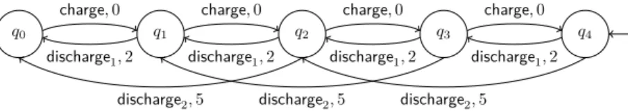
We depict SCAs in a fashion similar to the graphical representation of finite state automata: as a labeled graph, where vertices represent states and the edges transitions, labeled with elements of the CAS and c-semiring. The initial state is indicated by an arrow without origin. The CAS, c-semiring and threshold value will always be made clear where they are germane to the discussion. An example of an SCA is Ae, drawn in Figure 1; its CAS contains the incomposable actions charge, discharge1 and discharge2, and its c-semiring is the weighted semiringW. This particular SCA can model the component of the crop surveillance drone responsible for keeping track of the amount of energy remaining in the system; in stateqn (forn∈ {0,1, . . . ,4}), the drone hasnunits
of energy left, meaning that in statesq1toq4, the component can spend one unit of energy through
In statesq0 toq3, the drone can try to recharge throughcharge.2 Recall that, inW, higher values reflect a lower preference (a higherweight); thus,chargeis preferred overdischarge1.
q0 q1 q2 q3 q4
charge,0
discharge1,2
charge,0
discharge1,2
charge,0
discharge1,2
charge,0
discharge1,2
discharge2,5 discharge2,5 discharge2,5
Figure 1: A component modeling energy management,Ae.
Here, Ae is meant to describe the possible behavior of the energy management component
only. Availability of the actions within thetotal model of the drone (i.e., the composition of all components) is subject to how actions compose with those of other components; for example, the availability ofchargemay depend on the state of the component modelling position. Similarly, preferences attached to actions concern energy management only. In statesq0toq3, the component prefers to top up its energy level through charge, but the preferences of this component under composition with some other component may cause the composed preferences of actions composed with charge to be different. For instance, the total model may prefer executing an action that capturesdischarge2over one that captureschargewhen the former entails movement and the latter does not, especially when survival necessitates movement.
Nevertheless, the preferences ofAeaffect the total behavior. For instance, the weight of
spend-ing one unit of energy (throughdischarge1) is lower than the weight of spending two units (through
discharge2). This means that the energy component prefers to spend a small amount of energy before re-evaluating over spending more units of energy in one step. This reflects a level of care: by preferring small steps, the component hopes to avoid situations where too little energy is left to avoid disaster.
4.3
Composition
Composition of two SCAs arises naturally, as follows.
Definition 3. LetAi=
Qi,Σ,E,→i, q0i, ti
be an SCA fori∈ {0,1}. The(parallel) composition
ofA0 and A1 is the SCAQ,Σ,E,→, q0, t0⊗t1, denoted A0 ⊲⊳ A1, whereQ =Q0×Q1, q0 =
q0 0, q01
,⊗is the composition operator ofE, and →is the smallest relation satisfying
q0−−−−→0a0, e0 q0′ q1−−−−→1a1, e1 q1′ a0⊚a1 hq0, q1i−−−−−−−−−→ ha0a1, e0⊗e1 q0′, q1′i
In a sense, composition is a generalized product of automata, where composition of actions is mediated by the CAS: transitions with composable actions manifest in the composed automaton, as transitions with composed action and preference.
Composition is defined for SCAs that share CAS and c-semiring. Absent a common CAS, we do not know which actions compose, and what their compositions are. However, composition of SCAs with different c-semirings does make sense when the components model different concerns (e.g., for our crop surveillance drone, “minimize energy consumed” and “maximize covering of snapshots”), both contributing towards the overall goal. Earlier work on Soft Constraint Automata [20] explored this possibility. The additional composition operators proposed there can easily be applied to Soft Component Automata.
A stateqof a component may become unreachable after composition, in the sense that no state composed ofqis reachable from the composed initial state. For example, in the total model of our drone, it may occur that any state representing the drone at the far side of the field is unreachable, because the energy management component prevents some transition for lack of energy.
2
qY qN move,0
snapshot,0
move,2 pass,1 pass,1
Figure 2: A component modeling the desire to take a snapshot at every location,As.
q0,N q1,N q2,N q3,N q4,N
q0,Y q1,Y q2,Y q3,Y q4,Y
charge,1 charge,1 charge,1 charge,1
charge,1 charge,1 charge,1 charge,1
move2,5 move2,5 move2,5
snap shot1
,2
snap shot1
,2
snap shot1
,2
snap shot1
,2 move2,7 move2,7 move2,7
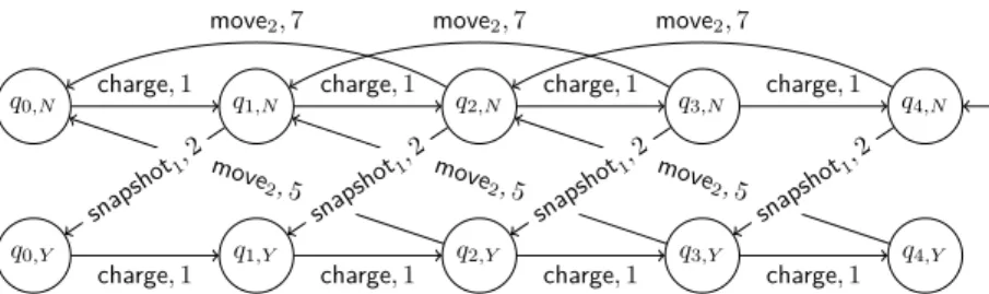
Figure 3: The composition of the SCAsAe and As, dubbedAe,s: a component modeling energy
and snapshot management. We abbreviate pairs of stateshqi, qjiby writingqi,j.
To discuss an example of SCA composition, we introduce the SCA As in Figure 2, which
models the concern of the crop surveillance drone that it should take a snapshot of every location before moving to the next. The CAS ofAs includes the pairwise incomposable actionspass,move
and snapshot, and its c-semiring is the weighted c-semiring W. We leave the threshold value ts undefined for now. The purpose ofAs is reflected in its states: qY (respectively qN) represents
that a snapshot of the current location was (respectively was not) taken since moving there. If the drone moves to a new location, the component moves toqN, whileqY is reached by taking a
snapshot. If the drone has not yet taken a snapshot, it prefers to do so over moving to the next spot (missing the opportunity).3
We grow the CAS of Ae and As to include the actionsmove, move2, snapshot and snapshot1 (here, the actionαi is interpreted as “execute actionαand account fori units of energy spent”),
and⊚is the smallest reflexive, commutative and transitive relation such that the following hold:
move⊚discharge2 (moving costs two units of energy), snapshot⊚discharge1 (taking a snapshot costs one unit of energy) andpass⊚charge(the snapshot state is unaffected by charging). We also choosemovedischarge2 =move2, snapshotdischarge1 =snapshot1 and passcharge= charge. The composition ofAe andAe is depicted in Figure 3.
The structure ofAe,s reflects that ofAe andAs; for instance, in stateq2,Y two units of energy
remain, and we have a snapshot of the current location. The same holds for the transitions ofAe,s;
for example,q2,N −−−−−−−→snapshot1,2 q1,Y is the result of composingq2 discharge1,2
−−−−−−−→q1andqN −−−−−−→snapshot,0 qY.
Also, note that inAe,s the preference of the move2-transitions at the top of the figure is lower than the preference of the diagonally-drawnmove2-transitions. This difference arises because the component transition inAsof the former isqN −−−−−→move,2 qN, while that of the latter isqY −−−−−→move,0 qN.
As such, the preferences of the component SCAs manifest in the preferences of the composed SCA. The actionsnapshot1is not available in states of the formqi,Y, because the only action available
inqY ispass, which does not compose intosnapshot1.
4.4
Behavioral semantics
The final part of our component model is a description of the behavior of SCAs. Here, the threshold determines which actions have sufficient preference for inclusion in the behavior. Intuitively, the threshold is an indication of the amount of flexibility allowed. In the context of composition, lowering the threshold of a component is a form of compromise: the component potentially gains behavior available for composition. Setting a lower threshold makes a component more permissive, but may also make it harder (or impossible) to achieve its goal.
The question of where to set the threshold is one that the designer of the system should answer
3
based on the properties and level of flexibility expected from the component; Section 5 addresses the formulation of these properties, while Section 6 talks about adjusting the threshold.
Definition 4. LetA=
Q,Σ,E,→, q0, t
be an SCA. We say that a stream σ∈Σωis abehavior
ofAwhen there exist streamsµ∈Qωandν∈Eω such thatµ(0) =q0, and for alln∈N,t≤ν(n) andµ(n) σ(n), ν(n)
−−−−−−−→µ(n+ 1). The set of behaviors of A, denoted byL(A), is called thelanguage
ofA.
We note the similarity between the behavior of an SCA and that of Büchi-automata [8]; we elaborate on this in Appendix A.
To account for states that lack outgoing transitions, one could include implicit transitions labelled with halt (and some appropriate preference) to an otherwise unreachable “halt state”, with a halt self-loop. Here, we set for all α ∈ Σ that halt⊚αand haltα = halt. To simplify matters, we do not elaborate on this.
Considerσ=hsnapshot,move,moveiω and τ =hsnapshot,move,passiω. We can see that when
ts = 2, both are behaviors of As; when ts = 1, τ is a behavior ofAs, while σis not, since every
secondmove-action in σhas preference 2. More generally, if Aand A′ are SCAs over c-semiring Ethat only differ in their threshold valuest, t′ ∈E, andt≤t′, thenL(A′)⊆L(A). In the case of
Ae, the threshold can be interpreted as a bound on the amount of energy to be spent in a single
action; ifte<5, then behaviors withdischarge2 do not occur inL(Ae).
Interestingly, if A1 and A2 are SCAs, then L(A1 ⊲⊳ A2) is not uniquely determined byL(A1) andL(A2). For example, suppose thatte = 4 and ts = 1, and considerL(Ae,s), which contains
hsnapshoti · hmove,snapshot,charge,charge,chargeiωeven though the corresponding stream of com-ponent actions inAe, i.e., the stream hdischarge1i · hdischarge2,discharge1,charge,charge,chargei
ω
is not contained in L(Ae). This is a consequence of a more general observation for c-semirings,
namely thatt≤eandt′ ≤e′ is sufficient but not necessary to derivet⊗t′ ≤e⊗e′.
5
Linear Temporal Logic
We now turn our attention to verifying the behavior of an agent, by means of a simple dialect of Linear Temporal Logic (LTL). The aim of extending LTL is to reflect the compositional nature of the actions. This extension has two aspects, which correspond roughly to the relations⊑and ⊚: reasoning about behaviors that capture (i.e., are composed of) other behaviors, and about behaviors that arecomposable with other behaviors. For instance, consider the following scenarios:
(i) We want to verify that under certain circumstances, the drone performs a series of actions where it goes north before taking a snapshot. This is useful when, for this particular property, we do not care about other actions that may also be performed while or as part of going north, for instance, whether or not the drone engages in communications while moving.
(ii) We want to verify that every behavior of the snapshot-component is composable with some behavior that eventually recharges. This is useful when we want to abstract away from the action that allows recharging, i.e., it is not important which particular action composes with
charge.
Our logic aims to accommodate both scenarios, by providing two new connectives: φ describes every behavior that captures a behavior validatingφ, while⊚φholds for every behavior composable with a behavior validatingφ.
5.1
Syntax and semantics
The syntax of the LTL dialect we propose for SCAs contains atoms, conjunctions, negation, and the “until” and “next” connectives, as well as the unary connectives⊚and . Formally, given a CAS Σ, the languageLΣis generated by the grammar
As a convention, unary connectives take precedence over binary connectives. For example,φ U¬ψ should be read as (φ)U(¬ψ). We use parentheses to disambiguate formulas where this convention does not give a unique bracketing.
The semantics of our logic is given as a relation|=Σbetween Σωand LΣ; to be precise, |=Σis the smallest such relation that satisfies the following rules
σ∈Σω
σ|=Σ⊤
σ∈Σω
σ|=Σσ(0)
σ|=Σφ σ|=Σψ
σ|=Σφ∧ψ
n∈N ∀k < n. σ(k)|=
Σφ σ(n)|=Σψ
σ|=Σφ U ψ
σ(1)|=Σφ
σ|=ΣX φ
σ6|=Σφ
σ|=Σ¬φ
σ|=Σφ σ⊑ωτ
τ |=Σφ
σ|=Σφ σ⊚ωτ
τ|=Σ⊚φ
in which⊑ω and⊚ωare the pointwise extensions of the relations⊑and⊚, i.e.,σ⊑ωτ when, for
alln∈N, it holds thatσ(n)⊑τ(n), and similarly for ⊚ω.
Although the atoms of our logic are formulas of the form φ = a ∈ Σ that have an exact matching semantics, in general one could use predicates over Σ. We chose not to do this to keep the presentation of examples simple.
The semantics of⊚andmatch their descriptions: ifσ∈Σω is described byφ(i.e.,σ|=Σφ) andτ ∈ Σω captures thisσ at every action (i.e.,σ ⊑ω τ), then τ is a behavior described by φ
(i.e.,τ |=Σφ). Similarly, ifρ∈Σωis described byφ(i.e.,ρ|=Σφ), and thisρis composable with
σ∈σω at every action (i.e.,σ⊚ωρ), thenρis described by⊚φ(i.e.,ρ|=
Σ⊚φ).
As usual, we obtain disjunction (φ∨ψ), implication (φ→ψ), “always” (φ) and “eventually” (♦φ) from these connectives. For example, ♦φ is defined as ⊤U φ, meaning that, if σ |=Σ ♦φ, there exists ann∈Nsuch that σ(n)|=Σφ. The operator⊚has an interesting dual that we shall consider momentarily.
We can extend |=Σ to a relation between SCAs (with underlying c-semiring E and CAS Σ) and formulas in LΣ, by defining A |=Σ φ to hold precisely when σ |=Σ φ for all σ ∈ L(A). In general, we can see that fewer properties hold as the thresholdt approaches the lowest preference in its semiring, as a consequence of the fact that decreasing the threshold can only introduce new (possibly undesired) behavior. Limiting the behavior of an SCA to some desired behavior described by a formula thus becomes harder as the threshold goes down, since the set of behaviors exhibited by that SCA is typically larger for lower thresholds.
We view the tradeoff between available behavior and verified properties as essential and desir-able in the design of robust autonomous systems, because it represents two options availdesir-able to the designer. On the one hand, she can make a component more accommodating in composition (by lowering the threshold, allowing more behavior) at the cost of possibly losing safety properties.
On the other hand, she can restrict behavior such that a desired property is guaranteed, at the cost of possibly making the component less flexible in composition.
Example: no wasted moves Suppose we want to verify that the agent never misses an oppor-tunity to take a snapshot of a new location. This can be expressed by
φw=(move→X(¬moveUsnapshot))
This formula reads as “every behavior captures that, at any point, if the current action is a move, then it is followed by a sequence where we do not move until we take a snapshot”. In-deed, if te⊗ts = 5, then Ae,s |=Σ φw, since in this case every behavior of Ae,s captures that
betweenmove-actions we find asnapshot-action. However, ifte⊗ts= 7, then Ae,s 6|=Σφw, since
hmove2,move2,charge,charge,charge,chargeiωwould be a behavior ofAe,s that does not satisfyφw,
as it contains two successive actions that capturemove.4 This shows the primary use of, which is to verify the behavior of a component in terms of the behavior contributed by subcomponents.
4
Example: verifying a component interface Another application of the operator⊚is to verify properties of the behavior composable with a component. Suppose we want to know whether all behaviors composable with a behavior ofA validateφ. Such a property is useful, because it tells us that, in composition, A filters out the behaviors of the other operand that do not satisfy φ. Thus, if every behavior that composes with a behavior ofAindeed satisfiesφ, we know something about the behaviorimposed byAin composition. Perhaps surprisingly, this use can be expressed using the ⊚-connective, by checking whether A|=Σ¬⊚¬φholds; for if this is the case, then for allσ, τ ∈ Σω with σ a behavior of A and σ⊚ωτ, we know that σ 6|=
Σ ⊚¬φ, thus in particular
τ6|=Σ¬φand thereforeτ |=Σφ.
More concretely, consider the component Ae. From its structure, we can tell that the action chargemust be executed at least once every five moves. Thus, ifτ is composable with a behavior ofAe, then τ must also execute some action composable withchargeonce every five moves. This
claim can be encoded by
φc=¬⊚¬ X⊚charge∨X2⊚charge∨ · · · ∨X5⊚charge
whereXndenotes repeated application ofX. IfAe|=Σφc, then every behavior ofAeis
incompos-able with behavior where, at some point, one of the next five actions is not composincompos-able with with
charge. Accordingly, ifσ∈Σωis composable with some behavior ofA
e, then, at every point inσ,
one of the next five actions must be composable withcharge. All behaviors that fail to meet this requirement are excluded from the composition.
5.2
Decision procedure
We developed a procedure to decide whetherA|=Σφholds for a given SCAA andφ∈ LΣ. The full details of this procedure are given in Appendix A; the main results are summarized below.
Proposition 1. Let φ ∈ LΣ. Given an SCA A and CAS Σ, the question whether A |=Σ φ is
decidable. In case of a negative answer, we obtain a stream σ ∈ Σπ such that σ ∈ L(A) but
σ6|=Σφ. The total worst-case complexity is bounded by a stack of exponentials in |φ|, i.e., 2. ..|φ|
, whose height is the maximal nesting depth of and⊚inφ, plus one.
This complexity is impractical in general, but we suspect that the nesting depth ofand⊚is at most two for almost all use cases. We exploit the counterexample in Section 6.
6
Diagnostics
Having developed a logic for SCAs as well as its decision procedure, we investigate how a designer can cope with undesirable behavior exhibited by the agent, either as a run-time behaviorσ, or as a counterexampleσto a formula found at design-time (obtained through Proposition 1). The tools outlined here can be used by the designer to determine the right threshold value for a component given the properties that the component (or the system at large) should satisfy.
6.1
Eliminating undesired behavior
A simple way to counteract undesired behavior is to see if the threshold can be raised to eliminate it — possibly at the cost of eliminating other behavior. For instance, in Section 5.1, we saw a formula
φw such thatAe,s6|=Σφw, with counterexampleσ=hmove2,move2,charge,charge,charge,chargeiω, when te⊗ts = 7. Since allmove2-labeled transitions of Ae,s have preference 7, raising5 te⊗ts to
5 ensures thatσ is not present in L(Ae,s); indeed, if te⊗ts = 5, then Ae,s |=Σ φw. We should be
careful not to raise the threshold too much: ifte⊗ts = 0, thenL(Ae,s) =∅, since every behavior
ofAe,s includes a transition with a non-zero weight — with thresholdte⊗ts= 0, Ae,s|=Σψholds forany ψ.
In general, since raising the threshold does not add new behavior, this does not risk adding additional undesired behavior. The only downside to raising the threshold is that it possibly
5
eliminates desirable behavior. We define the diagnostic preference of a behavior as a tool for finding such a threshold.
Definition 5. Let A =
Q,Σ,E,→, q0, t
be an SCA, and let σ ∈ Σπ∪Σ∗. The diagnostic
preferenceofσ inA, denoteddA(σ), is calculated as follows:
1. LetQ0be {q0}, and forn <|σ|setQn+1={q′:q∈Qn, q−−−−→σ(n), e q′}.
2. Letξ∈Eπ∪E∗ be the stream such thatξ(n) =L{
e:q∈Qn, q−−−−→σ(n), e q′}.
3. dA(σ) =V{ξ(n) :n≤ |σ|}, withV the greatest lower bound operator ofE.
Since σ is finite or eventually periodic, and Q is finite, ξ is also finite or eventually periodic. Consequently,dA(σ) is computable.
Lemma 2. Let A=
Q,Σ,E,→, q0, t
be an SCA, and let σ∈Σπ∪Σ∗. If σ∈L(A), or σ is a
finite prefix of someτ∈L(A), thent≤EdA(σ).
Proof. If σ ∈ L(A), there exist streams µ ∈ Qω and ν ∈ Eω such that µ(n) = q0, and for all
n∈ N, t ≤ν(n) and µ(n) σ(n), ν(n)
−−−−−−−→ µ(n+ 1). It is not hard to see that µ(n) ∈Qn for n ∈N.
Then also t ≤E ν(n) ≤E ξ(n) for alln ∈ N. Thus, t ≤E dA(σ). Likewise, ifσ is a finite prefix
of someτ ∈L(A), then t≤E dA(τ) by the above, and dA(τ)≤E dA(σ) by definition of dA, thus
t≤EdA(σ).
SincedA(σ) is a necessary upper bound ont whenσis a behavior ofA, it follows that we can
excludeσ from L(A) if we chooset such thatt6≤EdA(σ). In particular, if we choosetsuch that
dA(σ)<Et, then σ6∈L(A). Note that this may not always be possible: ifdA(σ) is1then such a
tdoes not exist.
Note that there may be another threshold (i.e., not obtained by Lemma 2), which may also eliminate fewer desirable behaviors. Thus, while this lemma gives helps to choose a threshold to exclude some behaviors, it is not a definitive guide. We refer to Appendix B for a concrete example.
6.2
Localizing undesired behavior
One can also use the diagnostic preference to identify the components that are involved in allowing undesired behavior. Let us revisit the first example from Section 5.1, where we verified that every pair ofmove-actions was separated by at least onesnapshotaction, as described inφw. Suppose we
choosete= 10 andts= 1; thente⊗ts = 11, thus σ=hmove2,charge,chargeiω∈L(As), meaning
Ae,s 6|=Σφw. By Lemma 2, we find that 11 =te,s =te⊗ts≤W dAe,s(σ) = 7. Even ifAs’s threshold
were as strict as possible (i.e.,ts = 0 =1W), we would find thatte⊗ts≤WdAe,s(σ), meaning that we cannot eliminate σby changing ts only. In some sense, we could say thatte is responsible for
σ.6
More generally, let (Ai)i∈I be a finite family of automata over the c-semiringEwith thresholds
(ti)i∈I. Furthermore, let A =
⊲⊳
i∈IAi and let ψ be such that A 6|=Σ ψ, with counterexample behaviorσ. Suppose now that for someJ ⊆I, we haveNi∈Jti ≤E dA(σ). Since ⊗is intensive, we furthermore know that N
i∈Iti ≤E Ni∈Jti. Therefore, at least one of ti for i ∈ J must be
adjusted to exclude the behaviorσ from the language of
⊲⊳
i∈IAi.We call (ti)i∈J suspect thresholds: some ti for i ∈ I must be adjusted to eliminate σ; by
extension, we refer to J as a suspect subset of I. Note that I may have distinct and disjoint suspect subsets. IfJ ⊆I is disjoint from every suspect subset ofI, thenJ is calledinnocent. IfJ
is innocent, changingtj for somej∈J (or eventj for allj∈J) alone does not excludeσ. Finding
suspect and innocent subsets of I thus helps in finding out which thresholds need to change in order to exclude a specific undesired behavior.
Algorithm 1 gives pseudocode to find minimal suspect subsets of a suspect set I; we argue correctness of this algorithm in Theorem 1; for a proof, see [19].
6
Arguably,Aeas a whole may not be responsible, because modifying the preference of themove-loop onqNinAs
FunctionFindSuspect(I):
M :=∅;
foreachi∈I do
if I\ {i} is suspect then
M :=M ∪FindSuspect(I\ {i}); end
end
if M =∅then return{I}; else
returnM; end
end
Algorithm 1:Algorithm to find minimal suspect subsets.
Theorem 1. If I is suspect and dA(σ)< 1, then FindSuspect(I) contains exactly the minimal
suspect subsets ofI.
Proof. First, note that it is easy to see thatFindSuspectnever returns∅.
The proof proceeds by induction onI. In the base, whereI ={i}, we can see thatN∅=1, thus, sincedA(σ)<1, it follows thatI\ {i}=∅is not suspect. The first branch of the subsequent
if is selected, which returns{I} itself. This matches the fact thatI is the only suspect subset of
I.
In the inductive step, we assume the claim holds for all strict subsets of I. We consider two cases. On the one hand, if there exists ani∈Isuch thatI\ {i}is suspect, then we know that the foreach-loop will modify M (since FindSuspectnever returns an empty set). Moreover,I itself is not minimally suspect. The algorithm then returns
[
{FindSuspect(I\ {i}) :i∈I, I\ {i} suspect}
By induction,FindSuspect(I\ {i}) returns all minimal suspect subsets ofI\ {i}. Since each of these is also a minimal suspect subset of I, and since very minimal suspect subset of I that is not equal toI is contained in one of these, the claim follows by the fact that we ruled outI as a minimal suspect subset.
In the case wheredA(σ) = 1, it is easy to see that{{i}:i∈I} is the set of minimal suspect
subsets ofI.
In the worst case, every subset ofIis suspect, and therefore the only minimal suspect subsets are the singletons; in this scenario, there areO(|I|!) calculations of a composed threshold value. Using memoization to store the minimal suspect subsets of everyJ ⊆ I, the complexity can be reduced toO(2|I|).
While this complexity makes the algorithm seem impractical (Ineed not be a small set), we note that the case where all components are individually responsible for allowing a certain undesired behavior should be exceedingly rare in a system that was designed with the violated concern in mind: it would mean thatevery component contains behavior that ultimately composes into the undesired behavior — in a sense,facilitating behavior that counteracts their interest.
7
Discussion
In this paper, we proposed a framework that facilitates the construction of autonomous agents in a compositional fashion. We furthermore considered an LTL-like logic for verification of the constructed models that takes their compositional nature into account, and showed the added value of operators related to composition in verifying properties of the interface between components. We also provided a decision procedure for the proposed logic.
this threshold to allow for more behavior, possibly to accommodate the preferences of another component, orincrease it to restrict undesired behavior observed at run-time or counterexamples to safety assertions found at design-time. We considered a simple method to raise the threshold enough to exclude a given behavior, but which may overapproximate in the presence of partially ordered preferences, possibly excluding desired behavior.
In case of a composed system, one can also find out which component’s thresholds can be thought of assuspectfor allowing a certain behavior. This information can give the designer a hint on how to adjust the system — for example, if the threshold of an energy management component turns out to be suspect for the inclusion of undesired behavior, perhaps the component’s threshold needs to be more conservative with regard to energy expenses to avoid the undesired behavior. We stress that responsibility may be assigned to a set of components as a whole, if their composed threshold is suspect for allowing the undesired behavior, which is possible when preferences are partially ordered.
8
Further Work
Throughout our investigation, the tools for verification and diagnosis were driven by the compo-sitional nature of the framework. As a result, they apply not only to the “grand composition” of all components of the system, but also to subcomponents (which may themselves be composed of sub-subcomponents). What is missing from this picture is a way to “lift” verified properties of subcomponents to the composed system, possibly with a side condition on the interface between the subcomponent where the property holds and the subcomponent representing the rest of the system, along the lines of the interface verification in Section 5.1.
If we assume that agents have low-latency and noiseless communication channels, one can also think of a multi-agent system as the composition of SCAs that represent each agent. As such, our methods may also apply to verification and diagnosis of multi-agent systems. However, this assumption may not hold. One way to model this could be to insert “glue components” that mediate the communication between agents, by introducing delay or noise. Another method would be to introduce a new form of composition for loosely coupled systems.
Finding an appropriate threshold value also deserves further attention. In particular, a method to adjust the threshold value at run-time, would be useful, so as to allow an agent to relax its goals as gracefully as possible if its current goal appears unachievable, and raise the bar when circumstances improve.
Lastly, the use soft constraints for autonomous agents is also being researched in a parallel line of work [31], which employs rewriting logic. Since rewriting logic is backed by powerful tools like Maude, with support for soft constraints [34], we aim to reconcile the automata-based perspective with rewriting logic.
A
Decision Procedure
In this appendix, we work out the details of a decision procedure for the logic proposed in Section 5, i.e., a procedure to decide whetherA|=Σφholds for a givenA andφ. This method follows [33], i.e., we do the following:
1. TranslateAto a Büchi-automatonAM with the same language asA.
2. Translateφto a Büchi-automatonAφ that accepts the streams verified byφ.
3. Check whether language ofAM is contained in that ofAφ.
The last step is an instance of checkingω-regular language containment, which can be decided inO(2|Aφ|), where|A
φ|is the number of states ofAφ[33]. Moreover, in case of a negative answer,
this method provides aσ∈Σπ such thatσ∈L(A
M) but σ6∈L(Aφ), and therefore σ∈L(A) but
σ6|=Σφ.
A.1
Büchi-automata
A(non-deterministic) Büchi-automaton [8] (BA) is a tupleA=
Q,Σ,→, q0, F
such thatQis a finite set ofstates, withq0∈Qtheinitial stateandF ⊆Qthe set ofaccepting states, Σ is a finite set called thealphabet and → ⊆Q×Σ×Qis a relation called the transition relation. We write
q a
−→q′ wheneverhq, a, q′i ∈ →.
A streamλ∈Qωis atrace of a streamσ∈Σω inAifλ(n) σ(n)
−−−→λ(n+ 1) holds for all n∈N. A traceλis accepting ifλ(n)∈F for infinitely manyn∈N. A streamσ∈Σωisaccepted byA if
it has an accepting traceλsuch thatλ(0) =q0. The set of streams accepted by Ais thelanguage
ofAand denoted byL(A).
AnAlternating Büchi-automaton (ABA) is a tupleA=
Q,Σ,→, q0, F
such thatQis a finite set of states with q0 ∈ Q the initial state and F ⊆ Q the set of accepting states, Σ is a finite set called the alphabet and → ⊆ Q×Σ×2Q is a (finite) relation called the transition relation.
Unlike a BA, a single transition in an ABA can have multiple destinations. We writeq a
−→P when
hq, a, Pi ∈ →. Arunof a streamσ∈ΣωinAis a labeled treeT such that the root ofT is labeled
withq0, and whenqis the label of a node ofT at depth nand the set of labels of children of said node is P, q σ(n)
−−−→P is a transition of A. A run T is accepting if every infinite branch of T is labeled by an accepting state infinitely often.
ABAs accept the same languages as their non-deterministic cousins [23]: given an ABAA, we can construct a BAA′ such thatL(A) =L(A′).
A.2
SCAs to a BAs
The translation of an SCA to a BA is relatively straightforward.
Lemma 3. LetA be an SCA. We can construct a BA A′ such that L(A) =L(A′). Proof. Choose A′ =
Q,Σ,→t, q0, Q, where →t is the relation in which q −→a t q′ if and only if
q a, e
−−→ q′ and t ≤e. We can now use the witness streams for σ∈ L(A) to show that σ∈ L(A′) and vice versa. Indeed, for the inclusion from right to left we can infer the existence of a stream
ν∈Eω, while for the inclusion from left to right we simply discard the stream of preferences.
A.3
Formulas to BAs
We present two methods to translate a formula into a BA that accepts precisely the streams validated by the formula. The first method is an extension of the recursive translation by Sherman et al. [29]. We also propose an extension to the approach of Muller et al. [24], which has a different complexity bound.
A.3.1 Recursive method
One easily constructs BAs that represent atomic formulas ⊤ and σ. Moreover, we can recreate the effect of logical connectives using BAs; for example, we can constructA such thatτ ∈L(A)
if and only if there exists aσ ∈L(A) with σ⊑ωτ easily: simply chooseA
=
Q,Σ,→, q0, F
where q b, e
−−→ q
′ if and only if q a, e
−−→ q′ with a ⊑ b. Similar constructions exist for the other connectives, including⊚. This is formalized in the following lemma.
Lemma 4. LetA1 andA2 be BAs over alphabetΣand leta∈Σ. One can construct BAsAa,A∧,
AU,AX,A¬,A andA⊚ such that the following are true
(i) σ∈L(Aa)if and only if σ(0) =a
(ii) σ∈L(A∧)if and only ifσ∈L(A1)andσ∈L(A2)[10]
(iii) σ ∈L(AU)if and only if there exists an n∈ N such that for all k < n, σ(k) ∈ L(A1) and
σ(n)∈L(A 2)
(iv) σ∈L(AX)if and only if σ′∈L(A
1)
(vi) σ∈L(A)if and only if τ⊑ωσfor someτ∈L(A1)
(vii) σ∈L(A⊚)if and only if σ⊚ωτ for some τ∈L(A
1)
Proof. We treat the claims one by one.
(i) The BAA=
{q0, q1},Σ,→, q0,{q1}
, where→is smallest relation such that q0 a
−→q1 and
q1 b
−
→q1 forb∈Σ, suffices.
(ii) Refer to [33, Proposition 6] for a proof.
(iii) Let Ai =Qi,Σ,→i, qi0, Fi for i ∈ {1,2} and assume (without loss of generality) that Q1 and Q2 are disjoint. We choose Q= Q1∪Q2∪ {q0} and F = F1∪F2, and let → be the smallest relation inQ×Σ×2Q satisfying the rules
i∈ {1,2} q a
−→iq
′
q a
−→ {q′}
q01 a
−→1q′
q0 a
−→ {q′, q0}
q02 a
−→2q′′
q0 a
−→ {q′′} We choose AU =
Q,Σ,→, q0, F
. It remains to show that AU validates the claim. If
σ ∈ L(AU), then there is an accepting run T of σ in AU. Let us refer to the nodes of T
labeled withq0 aspivot nodes. For everyn∈N, there is at most one pivot node at depthn, since every pivot node has a pivot node as its parent, and at most one pivot node among its children. Furthermore, there are two types of pivot nodes:
• nodes with children labeled byq0and someq′∈Q1, calledbranch nodes • nodes with children labeled by someq′′∈Q2, calledstop nodes
All children of stop nodes must be labeled with states inQ2; as a consequence, no stop node has a pivot node in its descendants. This shows that there is at most one stop node in T. Furthermore, if there were no stop nodes in T, then every pivot node would have a branch node among its children, rendering an infinite run of pivot nodes, which contradicts that T
is an accepting run. We can thus derive thatT has exactly one stop node at some depthn, and that all other pivot nodes inT occur as branch node parents of this stop node. One can then show that ifk < n, we can construct an accepting run forσ(k)inA
1 from the subtree of
T rooted at the unique branch node with depthk, and that the tree rooted at the stop node gives us an accepting run ofσ(n) inA
2.
For the other direction, one can combine the accepting runs ofσ(k)inA
1andσ(n)inA2into an accepting run ofσinAU easily, by starting with a finite tree consisting ofnpivot nodes,
and attaching the runs.
(iv) Simply add a new stateq to A1 and make this the initial state, then add a transition from
qto the initial state ofA1 labeled with afor everya∈Σ. It follows that σ∈L(AX) if and
only ifσ′ ∈L(A
1).
(v) Refer to [30] or [27] for a proof.
(vi) LetA1=Q1,Σ,→1, q01, F1. ChooseA=
Q1,Σ,→, q10, F1, where q−→b q
′ if and only if
there exists ana∈Σ such that q a
−→1q′ anda⊑b. It is easily shown that A validates the
claim.
(vii) By a construction analogous to the above.
We thus obtain a recursive formula-to-automaton translation; for example, if φ = ¬ψ, we construct the automatonAψ representingψ, from which we obtain the automatonAφrepresenting
φby the aforementioned construction.
Corollary 1. Let φ∈ LΣ. Then one can construct an automaton Aφ such that σ |=Σ φ if and