C
2013. The American Astronomical Society. All rights reserved. Printed in the U.S.A.
CLASH: COMPLETE LENSING ANALYSIS OF THE LARGEST COSMIC LENS
MACS J0717.5+3745 AND SURROUNDING STRUCTURES
∗Elinor Medezinski1, Keiichi Umetsu2, Mario Nonino3, Julian Merten4, Adi Zitrin5, Tom Broadhurst6,7, Megan Donahue8, Jack Sayers9, Jean-Claude Waizmann10, Anton Koekemoer11, Dan Coe11, Alberto Molino12, Peter Melchior13, Tony Mroczkowski4,9,24, Nicole Czakon9, Marc Postman11, Massimo Meneghetti10, Doron Lemze1,
Holland Ford1, Claudio Grillo14, Daniel Kelson15, Larry Bradley11, John Moustakas16, Matthias Bartelmann5,
Narciso Ben´ıtez12, Andrea Biviano3, Rychard Bouwens17, Sunil Golwala9, Genevieve Graves18, Leopoldo Infante19,
Yolanda Jim´enez-Teja6, Stephanie Jouvel20, Ofer Lahav21, Leonidas Moustakas4, Sara Ogaz11,
Piero Rosati22, Stella Seitz23, and Wei Zheng1
1Department of Physics and Astronomy, The Johns Hopkins University, 3400 North Charles Street, Baltimore, MD 21218, USA;[email protected] 2Institute of Astronomy and Astrophysics, Academia Sinica, P.O. Box 23-141, Taipei 10617, Taiwan
3INAF/Osservatorio Astronomico di Trieste, via G.B. Tiepolo 11, I-34143 Trieste, Italy 4Jet Propulsion Laboratory, California Institute of Technology, MS 169-327, Pasadena, CA 91109, USA
5Institut f¨ur Theoretische Astrophysik, Universit¨at Heidelberg, Zentrum f¨ur Astronomie, Philosophenweg 12, D-69120 Heidelberg, Germany 6Department of Theoretical Physics and History of Science, University of the Basque Country UPV/EHU, P.O. Box 644, E-48080 Bilbao, Spain
7Ikerbasque, Basque Foundation for Science, Alameda Urquijo, 36-5 Plaza Bizkaia, E-48011 Bilbao, Spain 8Department of Physics and Astronomy, Michigan State University, East Lansing, MI 48824, USA 9Division of Physics, Math, and Astronomy, California Institute of Technology, Pasadena, CA 91125, USA
10Dipartimento di Astronomia, Universit‘a di Bologna, via Ranzani 1, I-40127 Bologna, Italy 11Space Telescope Science Institute, 3700 San Martin Drive, Baltimore, MD 21208, USA
12Instituto de Astrof´ısica de Andaluc´ıa (CSIC), E-18080 Granada, Spain
13Center for Cosmology and Astro-Particle Physics and Department of Physics, The Ohio State University, Columbus, OH 43210, USA 14Dark Cosmology Centre, Niels Bohr Institute, University of Copenhagen, Juliane Mariesvej 30, DK-2100 Copenhagen, Denmark
15Observatories of the Carnegie Institution of Washington, Pasadena, CA 91101, USA 16Department of Physics and Astronomy, Siena College, 515 Loudon Road, Loudonville, NY 12211, USA
17Leiden Observatory, Leiden University, 2300-RA Leiden, The Netherlands
18Department of Astronomy, University of California, 601 Campbell Hall, Berkeley, CA 94720, USA 19Centro de Astro-Ingenier´ıa, Departamento de Astronom´ıa y Astrof´ısica, Pontificia Universidad Cat´olica de Chile,
V. Mackenna 4860, Santiago, Chile
20Institut de Ci´encies de l’Espai (IEEC-CSIC), E-08193 Bellaterra (Barcelona), Spain 21Department of Physics and Astronomy, University College London, London WC1E 6BT, UK
22ESO-European Southern Observatory, D-85748 Garching bei M¨unchen, Germany 23Universit¨ats-Sternwarte, M¨unchen, Scheinerstr. 1, D-81679 M¨unchen, Germany
Received 2013 April 3; accepted 2013 August 30; published 2013 October 15
ABSTRACT
The galaxy cluster MACS J0717.5+3745 (z = 0.55) is the largest known cosmic lens, with complex internal structures seen in deep X-ray, Sunyaev–Zel’dovich effect, and dynamical observations. We perform a combined weak- and strong-lensing analysis with wide-fieldBVRcizSubaru/Suprime-Cam observations and 16-bandHubble
Space Telescopeobservations taken as part of the Cluster Lensing And Supernova survey with Hubble. We find consistent weak distortion and magnification measurements of background galaxies and combine these signals to construct an optimally estimated radial mass profile of the cluster and its surrounding large-scale structure out to 5 Mpch−1. We find consistency between strong-lensing and weak-lensing in the region where these independent
data overlap, <500 kpch−1. The two-dimensional weak-lensing map reveals a clear filamentary structure traced
by distinct mass halos. We model the lensing shear field with nine halos, including the main cluster, corresponding to mass peaks detected above 2.5σκ. The total mass of the cluster as determined by the different methods is Mvir≈(2.8±0.4)×1015M. Although this is the most massive cluster known atz >0.5, in terms of extreme
value statistics, we conclude that the mass of MACS J0717.5+3745 by itself is not in serious tension withΛCDM, representing only a∼2σ departure above the maximum simulated halo mass at this redshift.
Key words: cosmology: observations – dark matter – galaxies: clusters: individual (MACS J0717.5+3745) – gravitational lensing: strong – gravitational lensing: weak
Online-only material:color figures
1. INTRODUCTION
In hierarchical structure formation theories, massive clusters are formed relatively recently and are still growing through the accretion of substructure. Accretion is predicted to occur
∗ Based in part on data collected at the Subaru Telescope, which is operated
by the National Astronomical Society of Japan.
24NASA Einstein Postdoctoral Fellow.
preferentially along filaments with clusters at the nodes of intersection (Bond et al.1996), a pattern which is now clearly visible in densely sampled large redshift surveys (Colless et al.
Table 1
Properties of the Galaxy Cluster MACSJ0717
Parameter Value
ID MACS J0717.5+3745
Optical position (J2000.0)
R.A. 07:17:32.63
Decl. +37:44:59.7
X-ray peak position (J2000.0)
R.A. 07:17:31.65
Decl. +37:45:18.5
Redshift 0.5458
X-ray temperature (keV) 12.5±0.7 Einstein radius () 60±3 atzs=2.963
Notes.The cluster MACS J0717.5+3745(z = 0.5458) was discovered in the MAssive Cluster Survey (MACS) as described by Reference (1), and its redshift determined by (2). The optical cluster center is defined as the center of the bright red-sequence selected galaxies. The X-ray center and mean temperature were taken from Reference (3). We note that the mean temperature can vary by larger than the quoted uncertainty between authors since it depends on the exact location of the X-ray center, which is different between (1) and (3).
References.(1) Ebeling et al.2001; (2) Ebeling et al.2007; (3) Postman et al.2012.
most luminous X-ray sources (Ebeling et al.2007) and strongest Sunyaev–Zel’dovich effect (SZE) signal (Planck Collaboration et al. 2011; Marriage et al. 2011; Vanderlinde et al. 2010). Selection effects are now understood to strongly favor the detection of gas compressed or shocked during cluster collision, as illustrated by hydrodynamical simulations (Ricker & Sarazin
2001; Burns et al.2008; Molnar et al.2012).
Large simulations of the growth of structure in the context of the standard cold dark matter (ΛCDM; Komatsu et al.2009) cosmological model have generated increasingly accurate pre-dictions for the evolution of the cluster mass function, extending to a limiting halo mass of approximately 2×10¹⁵M (Neto et al.2007; Duffy et al.2008; Zhao et al.2009; Bhattacharya et al. 2011). The number density of very massive clusters is predicted to change relatively rapidly at low redshift,z <1.0, where the evolution is principally sensitive to the cosmological matter density,Ωm. To a second order, one may hope to exam-ine the constancy with redshift expected for the “dark-energy” density (Allen et al.2004; Mantz et al.2008,2010b; Schmidt & Allen 2007) and test for self-consistency of general rela-tivity (Rapetti et al.2010). Presently, however, there are only indirect determinations of the masses of statistical samples of clusters, selected by X-ray means (Ebeling et al.2000,2001; Vikhlinin et al.2009a), and numbering only less than∼300 clus-ters, with masses mostly derived from uncertain X-ray scaling relations (Mantz et al.2010a; Vikhlinin et al.2006). Although these studies have not yet challenged the standard model (Mantz et al.2010b; Vikhlinin et al.2009b), much larger lensing-based surveys of clusters will eventually provide much more detail, in particular, the wide area Subaru/Hyper Suprime-Cam survey (Takada2010), and later Big-BOSS (Schlegel et al.2009), LSST (Ivezic et al.2008), Euclid (Laureijs et al.2011), and WFIRST (Green et al.2012).
Despite the lack of lensing-based cluster mass functions, we may progress by exploring the most extreme clusters (Owers et al.2011; Waizmann et al. 2012a; Colombi et al. 2011), in particular the most distant (Hoyle et al.2011), because of the exponential sensitivity of the cluster mass function to the growth of structure (Bahcall et al.1995; Chongchitnan & Silk 2012).
Anomalously large masses have been claimed for clusters at z1.5 (Rosati et al.2009; Jee et al.2009; Santos et al.2011; Foley et al.2011; Tozzi et al.2013). At lower redshifts, accurate full strong+weak lensing total masses were measured for the massive clusters such as A370 (z=0.375) and RX J1347.5 (z= 0.45), of the order of≈2–3×10¹⁵M
(Broadhurst et al.2008; Umetsu et al.2011a). These clusters were selected from all-sky X-ray surveys (Ebeling et al.2000,2001,2010), so that although the masses are larger and their redshifts are lower, the degree of tension withΛCDM is not extreme (Waizmann et al.2012a). At the present time, no individual cluster has been uncovered that strains the credibility of the standardΛCDM model.
Mapping the mass distribution in clusters has provided insight into the physics that govern dark matter (DM), the main mass component in the universe whose nature is largely unknown. The iconic “Bullet” cluster (Markevitch et al. 2002; Clowe et al. 2004) is an example of a post-merger cluster collision phase, where the diffuse gas component has been separated by ram-pressure from the DM and galaxies (Springel & Farrar
2007; Mastropietro & Burkert 2008), whereas lensing shows that the DM and the galaxies are still spatially coincident (Clowe et al.2006). This system serves to show that DM is effectively collisionless in nature. Subsequently, several new examples of bullet-like clusters have since been discovered with large-scale supersonic shock fronts (Markevitch et al. 2005; Menanteau et al.2012; Russell et al.2010; Korngut et al.2011; Macario et al.
2011; Owers et al.2011; Merten et al.2011; van Weeren et al.
2012), which are hard to reconcile with the expected pairwise velocity distribution of colliding galaxy clusters, where relative impact velocities in excess of 2000 km s−1 are unlikely in the context of ΛCDM (Lee & Komatsu 2010; Thompson & Nagamine2012).
To shed new light on these mysteries of DM and test struc-ture formation models with unprecedented precision, the Cluster Lensing And Supernova survey with Hubble (CLASH; Postman et al.2012),25a 524-orbitHubble Space Telescope(HST) multi-cycle treasury program, has been in progress to couple the lens-ing power of 25 massive clusters (Mvir = 5–30×1014M, ¯
zmed=0.4) withHSTin 16 passbands with full UV/optical/IR
coverage, complemented by Subaru wide-field imaging capabil-ities (e.g., Umetsu et al.2011a,2011b). Importantly, 20 CLASH clusters were X-ray selected to be relatively relaxed, in order to examine the concentration–mass relation for a sample with no strong selection bias toward high-concentration clusters. A fur-ther sample of five clusters were selected by their high lensing magnification properties, with the goal of detecting and study-ing high-redshift background galaxies magnified by the cluster potential.
MACS J0717.5+3745 (hereafter, MACSJ0717;z=0.5458) is one of the CLASH high-magnification clusters, and was originally detected by its X-ray emission, as part of the MAssive Cluster Survey (MACS; Ebeling et al.2001) and independently in the radio (Edge et al.2003). The cluster has the highest X-ray temperature in the MACS sample (kBTX =11.6 keV; Ebeling et al.2007; also see Table1), and has since been revealed as one of the most dynamically disturbed clusters known. In the core of this cluster, a complex four-component merging activity has been inferred from optical, X-ray, and internal dynamics (Ma et al. 2008, 2009). Low-frequency radio observations reveal very complex diffuse radio emission (Edge et al. 2003; van Weeren et al.2009; Bonafede et al.2009), indicative of a radio
relic or halo, and thought to be a signature of major mergers and common to many of the distant MACS clusters where large-scale supersonic shocks are found (Bonafede et al.2012). High-speed gas motion within MACSJ0717 is also tentatively inferred from dynamical data in a large spectroscopic study, where structural components were defined on the basis of X-ray emission peaks (Ma et al.2009). This high relative velocity has been confirmed in the multi-frequency SZE measurements of Mroczkowski et al. (2012), which deviate from a thermal SZE spectrum in a way that is consistent with kinetic SZE emission.
A strong-lensing (SL) analysis for this cluster has uncovered a complex elongated tangential critical curve encompassing the central substructures (Zitrin et al.2009a; Limousin et al.2012). In terms of the critical area, this cluster has the largest SL area, with an equivalent Einstein radius of,θE =55±3(at zs = 2.963), and an extremely large mass inside this region, M2D(<θE)∼ 7×10¹⁴M (Zitrin et al.2009a) was deduced. It has been argued that the size of the Einstein radius here may be inconsistent withΛCDM (Zitrin et al. 2009a; Meneghetti et al.2011). However, some studies (e.g., Oguri & Blandford
2009; Waizmann et al.2012b) showed that it can be explained as an extreme case in the context of the lens orientation or other effects. On the larger scale, MACSJ0717 was shown to be part of a filamentary structure from galaxy distributions (Ebeling et al.2004), and from weak-lensing (WL; Jauzac et al.2012), possibly spanning 4 Mpc in length.
In this paper, we aim to quantify the complex mass properties of MACSJ0717 and its surrounding large-scale structure (LSS) by employing a comprehensive weak and SL analysis based on deep, wide-field SubaruBV Rcizimaging, combined with our
recent CLASHHSTimaging. We use our methods to derive a robust total mass estimate, and calculate meaningful constraints on the existence of such rare high-mass peaks in a ΛCDM cosmology. The paper is organized as follows. In Section2, we describe the observational dataset, its reduction, and WL shape measurements. In Section3, we describe the selection of cluster and background galaxies for WL analysis. In Section 4, we present the WL analysis using Subaru observation. In Section5, we present improved SL analysis using our new CLASHHST observations, and in Section 6, we present a complementary WL analysis using theHSTobservations. In Section7, we derive cluster mass profiles from lensing, combining SL with WL shear and magnification measurements, and in Section8, we present the cluster mass distribution spanning both large scales and zooming in on the core, and constrain individual mass peaks using a multi-halo modeling approach. In Section9, we discuss our lensing mass properties, compare with complementary X-ray and SZE measurements, and contrast the cluster total mass we derive with predictions fromΛCDM cosmology using extreme value statistics. Finally, a summary of our work is given in Section10.
Throughout this paper, we use the AB magnitude system, and adopt a concordanceΛCDM cosmology withΩm =0.3,
ΩΛ = 0.7, andH0 =100h km s−1 Mpc−1 withh = 0.7. In
this cosmology, 1 corresponds to 268 kpc h−1 = 383 kpc at the cluster redshift,z = 0.5458. All quoted errors are 68.3% confidence limits (CL) unless otherwise stated. The center is taken as the mean location of red-sequence selected cluster members, R.A.=07:17:32.63, decl.= + 37:44:59.7 (J2000.0).
2. SUBARU+CFHT OBSERVATIONS
In this section, we present the data reduction and analysis of MACSJ0717 based on deep Subaru+CFHT multi-color images
Table 2
Subaru/Suprime-Cam + CFHT/MegaPrime Data
Filter Exposure Timea Seeingb m
limc
(ks) (arcsec) (AB mag)
u∗ 19.63 0.94 26.1
B 3.84 0.95 26.6
V 2.16 0.69 26.4
RCd 2.22 0.79 26.1
i 0.45 0.96 25.4
z 5.87 0.85 25.6
J 0.9 0.73 22.7
KS 0.5 0.54 23.0
Notes.
aTotal exposure time.
bSeeing FWHM in the full stack of images.
cLimiting magnitude for a 3σdetection within a 2aperture.
dBand used for WL shape measurements.
(Section2.1). We briefly describe our WL shape measurement procedure in Section2.2.
2.1. Data Reduction and Photometry
We analyze deepBV Rcizimages of MACSJ0717 observed
with the wide-field camera Suprime-Cam (34×27; Miyazaki et al.2002) at the prime focus of the 8.3 m Subaru Telescope. We observed the cluster on the night of 2010 March 17, in B, RC, z, to augment shallower observations that existed in the
Subaru archive, SMOKA.26 Some of the archival data for this cluster were taken as part of the “Weighing the Giants” program (von der Linden et al. 2012). The seeing full-widths at half-maximum (FWHMs) in the co-added mosaic images are 0.95 inB(3.84 ks), 0.69 inV(2.16 ks), 0.79 inRC(2.22 ks), 0.96 in
i(0.45 ks), and 0.85 inz(5.87 ks) with 0.20 pixel−1, covering
a field of approximately 36×34. The limiting magnitudes are obtained asB = 26.6,V =26.4,RC =26.1,i =25.4, and z=25.6 mag for a 3σ limiting detection within a 2diameter aperture.
To improve the accuracy of our photometric redshifts, we also include UV observations from the Megaprime/MegaCam in the u∗-band and near-IR observations from the WIRCAM in the J, Ks-bands on the Canada–France–Hawaii Telescope (CFHT), available from the CFHT archive.27Although shallower, and in the case of near-IR data the coverage is only of the inner 15×15, these extra bands add important information to help better constrain the spectral energy distribution (SED) of galaxies with degenerate fits.
The observation details of MACSJ0717 are listed in Table2. Figure1shows au∗BV Rcizcomposite color image
of the cluster central 28×28, produced automatically us-ing the publicly available Trilogy software (Coe et al.2012).28 We overlay it with the DM map determined from WL (white contours, see Section 8) and the smoothed X-ray luminosity map (red contours, see Section9.2).
Our reduction pipeline derives from Nonino et al. (2009) and SDFRED (Ouchi et al.2004; Yagi et al.2002) and has been op-timized for accurate photometry and WL shape measurements.
26 http://smoka.nao.ac.jp
27 This research used the facilities of the Canadian Astronomy Data Centre
operated by the National Research Council of Canada with the support of the Canadian Space Agency.
Figure 1.28×28CFHTu∗+SubaruBV Rcizcomposite color image showing
the galaxy cluster MACSJ0717 (z = 0.548). Overlaid are the surface mass density map reconstructed from our Subaru WL analysis (white contours) and the X-ray brightness map fromXMM-Newtonobservations (red contours). North is up and east is to the left.
(A color version of this figure is available in the online journal.)
Standard reduction steps include bias subtraction, flat-field cor-rection (super-flat averaged from all exposures of the same night where objects have been masked), and point-spread function (PSF) matching between exposures in the same band (if PSF variation is evident) as we normally use multi-epoch images taken under different conditions. Masking of saturated star trails and other artifacts is then applied.
To obtain an accurate astrometric solution for Subaru observa-tions, we retrieved processed MegaCamr-band (Filter Number: 9601) images from the CFHT archive and used it as a wide-field reference image. A source catalog was created from the co-added MegaCam rimage, using the Two Micron All Sky Survey catalog29as an external reference catalog. The extracted rcatalog has been used as a reference for the SCAMP software (Bertin2006) to derive an astrometric solution for the Suprime-Cam and other CFHT images. We do not use the CFHTr-band image in our photometry as the band is overlapping the Sub-aruRC band, but with much lower resolution and depth, and
therefore, does not carry added information.
For an accurate measure of photometry, we first smear the single exposures of the same band to the worst seeing. This step is done by using SDFRED/psfmatchprocedure, after suitable point-like sources have been previously selected. The WL band is chosen to be the band with a combination of best seeing and deepest observation,RCin this case (see Table2).
Finally, theSwarpsoftware (Bertin et al.2002) is utilized to stack the single exposures on a common world coordinate sys-tem grid with pixel-scale of 0.2 using the accurate registration
29 This publication makes use of data products from the Two Micron All Sky
Survey, which is a joint project of the University of Massachusetts and the Infrared Processing and Analysis Center/California Institute of Technology, funded by the National Aeronautics and Space Administration and the National Science Foundation.
that was achieved in the previous step. This assures minimal distortion of the final image. Note that for the WL band, we separately stack data collected at different epochs and different camera rotation angles.
The photometric zero-points for the co-added Suprime-Cam images were derived from a suitable set of reference stars identified in common with the calibrated MegaCam data. These zero-points were refined in two independent ways: first, by comparing with theHST/ACS magnitudes of cluster elliptical-type galaxies, translated to Subaru magnitudes using an elliptical SED template with the BPZ code; subsequently, by fitting SED templates with the BPZ code (Bayesian photometric redshift estimation; Ben´ıtez2000; Ben´ıtez et al.2004) to Subaru photometry of 12 galaxies having measured spectroscopic redshifts from the literature30 (Limousin et al. 2012) and calculating model magnitudes. This leads to a final photometric accuracy of∼0.01 mag in all passbands (see also Section3.3). The eight-band u∗BV RcizJ KS photometry catalog was then measured using SExtractor (Bertin & Arnouts 1996) in dual-image mode on PSF-matched images created by ColorPro (Coe et al.2006), where a combination ofB+V +R+zbands were used as a deep detection image (we exclude thei band which is of lesser quality). The stellar PSFs were measured from a combination of 100 stars per band and modeled usingIRAF
routines.
2.2. Subaru Shape Measurement
For shape measurements, we use our well-tested WL analysis pipeline based on the IMCAT package (Kaiser et al. 1995, KSB hereafter), incorporating modifications and improvements developed and outlined in Umetsu et al. (2010). Our KSB+ implementation has been applied extensively to Subaru cluster observations (e.g., Broadhurst et al.2005b,2008; Umetsu et al.
2007,2009,2010,2011a,2011b; Umetsu & Broadhurst2008; Okabe & Umetsu2008; Medezinski et al. 2010,2011; Zitrin et al.2011,2013; Coe et al. 2012; Umetsu et al. 2012). Full details of our CLASH WL analysis pipeline are presented in Umetsu et al. (2012).
Based on simulated Subaru Suprime-Cam images (see Section 3.2 of Oguri et al. 2012; Massey et al. 2007a), we found in our earlier work (Umetsu et al.2010,2012) that the WL signal can be recovered with|m| 5% of the multiplica-tive shear calibration bias (as defined by the STEP project: see Heymans et al.2006; Massey et al.2007a), andc ∼ 10−3 of the residual shear offset, which is about one order of magnitude smaller than the typical distortion signal in cluster outskirts (|g| ∼10−2). Accordingly, we include in our analysis a
calibra-tion factor of 1/0.95 asgi → gi/0.95 to account for residual calibration.31
In this analysis, we use theRC-band data taken in 2005 and 2010, which have the best image quality in our datasets, taken in fairly good seeing conditions. Two separate co-addedRC-band images are created, one from 2005 (with a total of 450 s, observer Yasuda) and one from 2010 (with a total of 2160 s, observed by us on 2010 March). We do not smear the single exposures before
30 This research has made use of the NASA/IPAC Extragalactic Database
(NED) which is operated by the Jet Propulsion Laboratory, California Institute of Technology, under contract with the National Aeronautics and Space Administration.
31 Our earlier CLASH weak-lensing work in Zitrin et al. (2011), Umetsu et al.
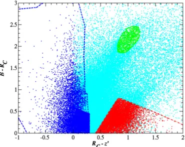
Figure 2.“Blue” and “red” background galaxies are selected for WL analysis (lower left blue dashed and right red dot-dashed contours, respectively) based on SubaruB, RC, zcolor–color–magnitude selection. All galaxies (cyan) are
shown in the diagram. At small clustercentric radius, an overdensity of cluster galaxies defines our “green” sample (green solid contour), comprising mostly the red sequence of the cluster and some blue trail of later type cluster members. The background samples are well isolated from the green region and satisfy other criteria as discussed in Section3.2.
(A color version of this figure is available in the online journal.)
stacking (as done for photometric measurements), so as not to degrade and destroy the WL information derived from the shapes of galaxies. A shape catalog is created for each epoch separately, and the catalogs themselves are then combined by properly weighting and stacking the calibrated distortion measurements for galaxies in the overlapping region. The combination of both epochs increases the number of measured galaxy shapes and improves the statistical measurement, while not degrading the quality of the shape measurement due to different seeing and anisotropy at different observing epochs.
3. SAMPLE SELECTION
For an undiluted WL detection, we need to carefully select a pure sample of background galaxies. In order to further explore the distribution of the cluster galaxies, we also identify the cluster members population. We use theB, Rc, z Subaru
imaging which spans the full optical wavelength range to perform color–color (CC) selection of cluster and background samples, as demonstrated by Medezinski et al. (2010) and detailed below.
3.1. Cluster Sample Selection
In Figure2, we show theB−RCversusRC−zdistribution
of all galaxies to our limiting magnitude (cyan). To identify our cluster-dominated area in this CC space, we also plot upB−Rc versusRC−z only of galaxies with small projected distance
R < 3 (1 Mpc at zl = 0.546) from the cluster center. A region is then defined according to a characteristic overdensity in this space (shown as a solid green curve in Figure2). Then,all galaxies within this distinctive region from the full CC diagram define the “green” sample (green points in Figure2), comprising mostly the red-sequence of the cluster and a blue trail of later-type cluster members. We note that the small overdensity seen bluer (lower-left,B−RC, RC−z∼0.7) than our green sample does not lie at the same redshift of the cluster and is not a bluer
population that is part of the cluster, but is in fact comprised of early-type galaxies lying in the foreground of the cluster, at about z ∼ 0.33, which we will discuss further as part of our multi-halo mass modeling (Section8.2).
The number density profile of the green sample is steeply rising toward the center (Figure 6, green crosses). The low number density at large clustercentric radius is indicative of negligible contamination of background galaxies of this sample. The WL signal for this population is found to be consistent with zero at all radii (Figure 5, green crosses), also indicating the reliability of our procedure. For this population of galaxies, we find a mean photometric redshift of zphot ≈ 0.56 (see
Section3.3), consistent with the cluster redshift. Importantly, the green sample marks the region that contains a majority of unlensed galaxies, relative to which we select our background samples, as summarized below.
3.2. Background Sample Selection
A careful background selection is critical for a WL analysis so that unlensed cluster members and foreground galaxies do not dilute the true lensing signal of the background (Broadhurst et al.2005b; Medezinski et al.2007,2010; Umetsu & Broadhurst
2008). This dilution effect is simply to reduce the strength of the lensing signal when averaged over a local ensemble of galaxies (by a factor of 2–5 atR 400 kpch−1; see Figure 1
of Broadhurst et al. 2005b), particularly at small radii where the cluster is relatively dense, in proportion to the fraction of unlensed galaxies whose orientations are randomly distributed. We use the background selection method of Medezinski et al. (2010) to define undiluted samples of background galax-ies, which relies on empirical correlations for galaxies in color–color–magnitude space derived from the deep Subaru photometry, by reference to evolutionary tracks of galaxies (for details, see Medezinski et al.2010; Umetsu et al.2010) as well as to the deep photometric-redshift survey in the COSMOS field (Ilbert et al.2009).
For MACSJ0717, we have a wide wavelength coverage (BV Rciz) of Subaru/Suprime-Cam. We therefore make use
of the (B −Rc) versus (Rc−z) CC diagram to carefully
select two distinct background populations which encompass the red and blue branches of galaxies. We limit the red sample to z<25 mag in the reddest band, corresponding approximately to a 5σ limiting magnitude within 2 diameter aperture. We extend the magnitude limit of the blue samples further to z < 26 mag, where the number density of galaxies grows significantly higher, especially for bluer galaxies whose faint-end slope of the luminosity function is rising, giving a much improved WL statistical measurement.
For the background samples, we define conservative color limits, where no evidence of dilution of the WL signal is visible, to safely avoid contamination by unlensed cluster members and foreground galaxies. The color boundaries of our “blue” and “red” background samples are shown in Figure2. For both the blue and red samples, we find a consistent, rising WL signal (see Section4.1) all the way to the center of the cluster, as shown in Figure5.
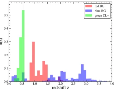
Figure 3.Redshift distributions of the CC-selected green, red, and blue samples using the BPZ photo-z’s based on Subaru+CFHT imaging. The cluster redshift is marked with a black line.
(A color version of this figure is available in the online journal.)
Table 3
Galaxy Color Selection
Sample Magnitude Limitsa N n
gb zsc
(AB mag) (arcmin−2)
Red 21< z<25 10490 9.6 1.21
Green z<24 1252 1.3 0.49/0.54
Blue 22.5< z<26 11998 11.5 2.23
Notes.
aMagnitude limits for the galaxy sample.
bMean surface number density of source background galaxies. cMean photometric redshift of the sample obtained with the BPZ code.
the cluster center, caused by the lensing magnification effect. A more quantitative magnification analysis is given in Section4.2. To summarize, our CC selection criteria yielded a total of N=10,490, 1252, and 11,998 galaxies, for the red, green, and blue photometry samples, respectively (see Table3). For our WL distortion analysis, we have a subset of 4856 and 4738 galaxies in the red and blue samples (with usable RC shape
measurements), respectively (see Table4).
3.3. Depth Estimation
The lensing signal depends on the source redshiftzsthrough the distance ratioβ(zs) = Dls/Ds, whereDls,andDs are the
angular diameter distances between the lens and the source, and the observer and the source, respectively. We thus need to estimate and correct for the respective depthsβof the different galaxy samples when converting the observed lensing signal into physical mass units.
For this, we utilize BPZ to measure photometric redshifts (photo-zs)zphotusing our deep Subaru+CFHTu∗BV RcizJKs
photometry (Section2.1). BPZ employs a Bayesian inference where the redshift likelihood is weighted by a prior probability, which yields the probability densityP(z, T|m) of a galaxy with apparent magnitudemof having certain redshiftzand spectral typeT. In this work, we used a new library (N. Benitez 2012, in preparation) composed of 10 SED templates originally from PEGASE (Fioc & Rocca-Volmerange 1997) but recalibrated using the FIREWORKS photometry and spectroscopic redshifts
Figure 4.Lensing depth (Dls/Ds) as a function of Subaruz-band limiting
magnitude for the red and blue background samples, as estimated from the photometric redshifts of COSMOS toz<25 (circles). In order to estimate the depth of the blue sample to its limiting magnitude ofz<26,we extrapolate the curve (x’s).
(A color version of this figure is available in the online journal.)
from Wuyts et al. (2008) to optimize its performance. This library includes five templates for elliptical galaxies, two for spiral galaxies, and three for starburst galaxies. In our depth estimation, we utilize BPZ’s ODDS parameter, which measures the amount of probability enclosed within a certain intervalΔz centered on the primary peak of the redshift probability density function, serving as a useful measure to quantify the reliability of photo-zestimates.
We only consider galaxies from the WL-matched catalogs, as those are the galaxies from which we estimate the lensing signal and finally, the mass profile. To make this estimate more robust, we use galaxies for which the photo-zwas determined using all available eight bands. We show the normalized redshift distribution of these galaxies in each of the green, red, and blue samples in Figure 3. Still, since only 12 spectroscopic redshifts are publicly available in this field, it is difficult to estimate the reliability of our photo-z’s. Therefore, we further compare our results with the more reliably estimated depths we derive from the COSMOS catalog (Ilbert et al.2009), which has robust photometry and photo-zmeasurements for the majority of galaxies withi <25 mag. For each sample, we apply the same CC selection to the COSMOS photometry and obtain the redshift distributionN(z) of field galaxies. Since COSMOS is only complete toi <25 mag, we derive the mean depth as a function of magnitude (Figure4) up to that limit, and extrapolate to our sample limiting magnitude,z=25 in the case of the red sample andz=26 in the case of the blue sample.
For each background population, we calculate a weighted mean of the distance ratioβ(mean lensing depth) as
β =
dz w(z)N(z)β(z)
dz w(z)N(z) , (1)
where w(z) is a weight factor; wis taken to be the Bayesian ODDS parameter for the BPZ method, and w = 1 other-wise. The sample mean redshift zs is defined similarly to Equation (1).
Table 4
Galaxy Samples for WL Shape Measurements
Sample N nga σgb zs,effc Dls/Dsd
(arcmin−2) MACSJ0717 COSMOS MACSJ0717 COSMOS
Red 4856 5.65 0.41 1.1 1.08 0.43 0.42
Blue 4738 5.6 0.42 1.89 1.56 0.59 0.55
Blue+red 9594 11.2 0.41 1.26 1.27 0.48 0.48
Notes.
aMean surface number density of galaxies. bMean rms error for the shear estimate per galaxy,σ
g≡(σg2)1/2.
cEffective source redshift corresponding to the mean depthβof the sample. dDistance ratio averaged over the redshift distribution of the sample,β.
For each background sample, we obtained consistent mean-depth estimates β (within 2%) using the BPZ- and COSMOS-based methods. In the present work, we adopt a conservative uncertainty of 5% in the mean depth for the com-bined blue and red sample of background galaxies,β(back) = 0.48 ± 0.03, which corresponds to zs,eff = 1.26 ± 0.1.
We marginalize over this uncertainty when fitting parameter-ized mass models to our WL data.
4. SUBARU WEAK-LENSING ANALYSIS
In this section, we describe the WL analysis based on our deep Subaru imaging data. In Section4.1, we derive cluster lens distortion, and in Section4.2, we derive the magnification radial profiles from the data.
4.1. Tangential Distortion Analysis
The shape distortion of an object is described by the complex reduced-shear,g=g1+ig2, where the reduced-shear is defined as (in the subcritical regime; see, e.g., Bartelmann & Schneider
2001)
gα≡γα/(1−κ), (2)
where γ is the complex gravitational shear field and is non-locally related to the convergence,κ = Σ/Σcrit, which is the
surface mass density in units of the critical surface-mass density for lensing,Σcrit=(c2/4π GDl)β−1. The tangential component
of the reduced-shear, g+, is used to obtain the azimuthally
averaged distortion due to lensing, and computed from the distortion coefficients (g1, g2):
g+= −(g1cos 2θ+g2sin 2θ), (3)
whereθ is the position angle of an object with respect to the cluster center. The uncertainty in the objectg+ measurement
is σ+ = σg/
√
2 ≡ σ in terms of the rms error σg for the complex reduced-shear measurement. For each galaxy, σg is the variance for the reduced shear estimate computed from 50 neighbors identified in the rg–RC plane. To improve
the statistical significance of the distortion measurement, we calculate the weighted average ofg+
g+,i≡g+(θi)=
k∈i
w(k)g+(k)
k∈i w(k)
−1
, (4)
where the indexkruns over all objects located within theith radial bin with a weighted center ofθi, andw(k) is the weight
for thekth object,
w(k) =1/
σg2(k)+α2, (5)
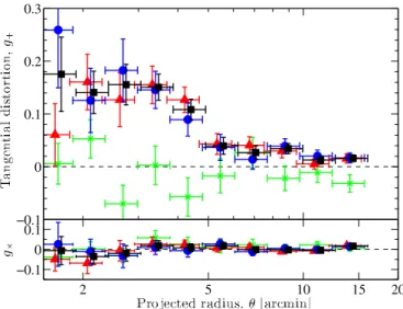
Figure 5.Azimuthally averaged radial profiles of the tangential reduced-shear
g+(upper panel) and the 45◦rotated (×) componentg×(lower panel) for our red (triangles), blue (circles), green (crosses), and blue+red (squares) galaxy samples. The symbols for the red and blue samples are horizontally shifted for visual clarity. For all of the samples, the×-component is consistent with a null signal detection well within 2σat all radii, indicating the reliability of our distortion analysis.
(A color version of this figure is available in the online journal.)
whereα2is the softening constant variance. We chooseα=0.4, which is a typical value of the mean rmsσg¯ over the background sample. The uncertainty ing+,i is calculated from a bootstrap error analysis (for details, see Umetsu et al.2012). Since WL only induces curl-free tangential distortions, the 45◦ rotated component, g× = −(g2cos 2φ −g1sin 2φ), is expected to
vanish. It is therefore useful as a check for systematic errors. In Figure 5, we plot the radial profile of g+ of the green,
red, and blue samples defined above. The black points represent the red+blue combined sample (also shown in Figure8, upper panel), showing the best estimate of the lensing signal, which is detected at 11.6σ significance over the full radial range. The red and blue sample profiles rise continuously toward the center of the cluster, and agree with each other within the errors, except at the very central bin,θ 2, where measurements are approaching the nonlinear regime, given the extremely elliptical shape of the tangential critical curve (see Figure 1 of Zitrin et al.
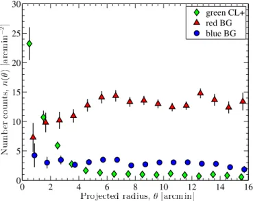
Figure 6. Surface number density profiles n(θ) of Subaru BRcz-selected
samples of galaxies. The red (triangles) and blue (circles) samples comprise background galaxies, and the green (crosses) sample comprises mostly cluster galaxies, as is evident by their steeply rising number counts toward the center. See also Figure8.
(A color version of this figure is available in the online journal.)
4.2. Magnification-bias Analysis
We follow the prescription of Umetsu et al. (2011a) to measure the magnification bias signal as a function of distance from the cluster center, which depends on the intrinsic slope of the luminosity function of background sourcess, as
nμ(θ)=n0μ(θ)2.5s−1, (6)
where n0 = dN0(<mcut)/dΩ is the unlensed mean number
density of background sources for a given magnitude cutoff mcut, approximated locally as a power-law cut with slope,
s = dlog10N0(<m)/dm > 0. We use the red sample of background galaxies (Section3.2), for which the intrinsic count slopesat faint magnitudes is relatively flat,s ∼0.1, so that a net count depletion results (Broadhurst et al.2005b; Umetsu & Broadhurst2008; Umetsu et al.2010,2011a). In contrast, the blue background population has a steeper intrinsic count slope close to the lensing invariant slope (s=0.4).
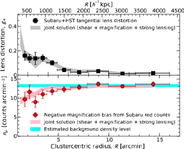
Here we use the approach developed in Umetsu et al. (2011a) to measure the azimuthally averaged surface number density profile of the red galaxy counts,nμ,i ≡ nμ(θi) (red triangles in Figure 6), taking into account and correcting for masking of background galaxies due to bright cluster galaxies (BCGs), foreground objects, and saturated objects. The errorsσμ,i for nμ,iinclude both contributions from Poisson errors in the counts and contamination by intrinsic clustering of red background galaxies. The normalization and slope parameters for the red sample are reliably estimated outside the lensed region, by virtue of the wide-field imaging with Subaru/Suprime-Cam. We find n0=13.3±0.3 galaxies acrmin−2ands=0.123±0.048.
In the bottom panel of Figure 8, we show the measured magnification profile from our flux-limited sample of red background galaxies (z < 25 mag; see Table 3) with and without the masking correction applied (red circles and green crosses, respectively). A clear depletion of the red counts is seen in the central, high-density region of the cluster and detected out to 4 from the cluster center. The radially integrated significance of the detection of the depletion signal is 5.3σ.
The high-level WL shear and magnification profile we de-rived here can be combined together to reconstruct the under-lying mass profile. However, to better resolve the core of the profile, we require further constraints which are enabled by SL. Therefore, we derive the SL mass profile in the next section.
5.HSTSTRONG-LENSING ANALYSIS
For a massive cluster, the weak- and strong-regimes con-tribute similar logarithmic coverage of the mass profile. Hence, the central SL information is crucial in a cluster lensing analysis (Umetsu et al.2011a,2011b,2012). In this section, we derive an SL model to compare with our WL profile in the overlap region and to combine with WL in deriving the mass reconstruction in Section7.
First, we summarize our well-tested approach to strong-lens modeling, developed by Broadhurst et al. (2005a) and optimized further by Zitrin et al. (2009b) (see also Zitrin et al.2013). Briefly, the adopted parameterization is as follows. Cluster members, chosen by a F814W-F555W color criterion, are each represented by a power-law mass density profile. The superposition of all galaxy contributions constitutes the galaxy, lumpy component for the model. This component is then smoothed using a two-dimensional (2D) spline interpolation to comprise the DM component. The two components are then added with a relative weight. In order to allow further degrees of freedom (dof), and higher effective ellipticity of the critical curves, an external shear is added. In total, the method thus includes six basic free parameters: (1) the power-law of the galaxy mass profile; (2) the smoothing (polynomial) degree of the DM component; (3) the relative weight of the galaxy to the DM component; (4) the overall scaling or normalization; (5) the amplitude; and (6) angle of the external shear (for more details see Zitrin et al.2009b).
Using this method, in Zitrin et al. (2009a), we performed the first SL analysis of this cluster using three-band publicly available HST imaging, and found 34 multiple-images from 13 lensed sources, uncovering that MACSJ0717 is the largest known lens. As part of CLASH (Postman et al.2012), we further observed MACSJ0717 withHSTin 16 filters with the Advanced Camera for Surveys (ACS) and WFC3/UVIS+IR cameras. We thus revise here our primary multiple image identification, and follow in general the multiple image sets listed in Table 1 of Limousin et al. (2012, hereafter L12), who recently used Zitrin et al.’s (2009a) systems (with the exclusion of three systems, 9–11) and added five additional multiple systems which were subsequently verified with the help of the publicly available CLASH WFC3/IR images. Although we agree with most of the identifications and revisions byL12, we determine image 1.5 to be at a different location, R.A. =07:17:37.393, decl.=+37:45:40.90. We also confirm that this new location significantly improves the SL parametric solution ofL12 (M. Limousin 2013, private communication). In addition, although the model suggests these may be counter images of the same source, we omit system 2 from our list, since it strongly deviates from theDls/Ds scaling relation expected, and as determined
We use a several dozen thousand step Monte Carlo Markov Chain (MCMC) minimization in order to find the best-fit solution, defined by the image-plane reproduction χ2. The advantage of this light-traces-mass (Zitrin et al.2009a) method is that even very complex systems such as MACSJ0717 are still well fitted by this simple procedure, although it may not be expected to yield an rms as low as in a multi-halo/parametric fit (e.g.,L12). Note, however, that even with a somewhat higher rms, the representation is still highly credible as it allowed the identification of many multiple image systems (Zitrin et al.
2009a).
Here, in practice, to allow for more freedom and a better rms, we also leave the relative weight of 10 galaxies to be freely optimized by the MCMC. With this, the final model we present here has an rms of 3.86 and a χ2 of 334 (with a
location error ofσ = 1.4), over 32 dof. The relatively large reducedχ2 (compared with the reasonable rms) may indicate
that in such a complex system, a position error of 1.4 may be underestimated, not taking into account stronger LSS and complexity effects. Since the best-fit statistical solution defined by the image positions may not always reproduce the multiple images with the right internal shape or orientation, multiple images are then sent to the source plane and back through the lens to test, by eye, the reproduction of other multiple images of the same systems (e.g., Zitrin et al.2009a,2009b). Note that only five systems have spectroscopic redshift, so that we use the input fromL12as the predicted redshift of the other systems. We do not leave any of these redshifts to be optimized by the model, which may have further lowered the rms of our model.
We present the azimuthally averaged projected mass density profile from the resulting SL model of MACSJ0717 in Figure13
(green curve). The density profile shows a remarkably flat core out to180 kpch−1, as was noted in previous SL analyses of this
cluster (Zitrin et al.2009a). The shallow profile is in accordance with the non-relaxed appearance of this cluster and reported multiple mass clumps at the core of the cluster. According to our SL model, the total projected mass enclosed within a radius of 60 ±6, the effective Einstein radius at zs = 2.963, is M2D(<60)=(4.87±0.35)×1014Mh−1, which is in good
agreement with the mass enclosed within the tangential critical curve,M2D=(5.5±0.35)×1014M
h−1. We now turn to the WL analysis in the next sections in order to recover the mass over the full scale of the cluster.
6.HSTWEAK-LENSING ANALYSIS
In order to further constrain the mass profile in the cluster center, where the small Subaru number density leads to large uncertainties, we perform a complementary WL analysis of the HST16-band data in the weak regime. Details of our reduction, photometry, and photo-zpipeline were given in previous papers (Postman et al.2012; Zitrin et al.2012b; Coe et al.2012). Here we further produced specialized drizzled images, optimized for WL, consisting of drizzling each visit in the “unrotated” frame of the ACS/WFC3 detectors, using a modified version of the “Mosaicdrizzle” pipeline (described more fully in Koekemoer et al. 2011). This allows accurate PSF treatment that does not compromise the intrinsic shape measurements required by WL pipelines. The RRG (Rhodes et al.2000) WL shape measurement package was then used to measure shapes in each of six ACS bands (F435W, F475W, F625W, F775W, F814W, and F850LP), and the DEIMOS (Melchior et al.2011) package was used to measure shapes in the WFC3/IR F160W band. We exclude objects with signal-to-noise ratio (S/N)<10 and size
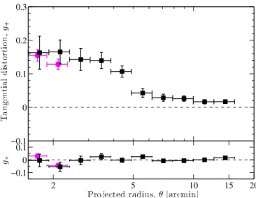
Figure 7.As in Figure 5, we show the tangential distortion profile of the Subaru background sample (black squares), and compare with theHST-derived background sample in the centralR <2.4 (magenta circles) but outside the critical lensing region,R >1.5. As can be seen, these two complementary datasets give consistent WL signal at the region of overlap, whereas theHST points have much smaller errors and therefore provide better constraints. (A color version of this figure is available in the online journal.)
<0.1. All of the shape catalogs were then matched to the deep multi-band photometric catalog and merged where there was more than one shape measurement per object, using its S/N as input weight of each measurement, according to Equation (5) withα=0.2 as the softening kernel in this case.
Since theHSTfield has reliable photometric redshifts mea-sured from 16 bands spanning UV to IR, here we rely on those for a secure selection of background galaxies. We define our background sample as galaxies having 0.8< zb <4, zb,min >
0.6, zb,max < 5,22.5 < mF625W < 27.5, where zb is the
Bayesian photometric redshift from BPZ, andzb,minandzb,max
are the 68% lower and upper bound on the photometric red-shift estimate, respectively. To examine the light distribution, we chose an inclusive cluster-member sample based on|zb−zcl|<
0.1, zb,min > zcl−0.2, zb,max< zcl+0.2,17< mF625W <24.5. In order to do a simultaneous analysis of the WL signal in both theHSTand Subaru fields, we need to account for the differ-ent redshift distribution of the differdiffer-ent populations these two datasets target. We do this by estimating the depth factor,β(z), from the HSTphoto-z’s. For theHSTbackground catalog we estimateβ ∼ 0.525, about a∼10% increase in depth relative to the Subaru catalog, estimated at β ∼ 0.48. We apply this relative correction to theHSTcatalog and scale it to match the Subaru catalog.
is still negligible and does not significantly affect our results. We will present the 2D distribution analysis of theHSTregion in Section8.4, after we first incorporate theHST+Subaru WL withHSTSL information to reconstruct the mass profile over the entire Subaru field of view (FOV) in the next section.
7. RADIAL MASS PROFILE ANALYSIS
7.1. Mass Profile Reconstruction Using One-dimensional Shear and Magnification
We derive the cluster mass profile as a function of clus-tercentric radius from a joint likelihood analysis of inde-pendent WL distortion (g+), magnification-bias (nμ), and SL
projected mass (m) constraints,{g+,i}iN=wl1(Section4.1),{nμ,i}
Nwl
i=1
(Section 4.2), and {mi}Nsl
i=1 (Section 5), respectively,
follow-ing the Bayesian approach of Umetsu (2013), who extended theshear-and-magnificationanalysis method of Umetsu et al. (2011a) to include the inner SL information. Such a multi-probe approach is critical for improving the accuracy and pre-cision of the cluster lens reconstruction, effectively breaking the mass-sheet degeneracy (see Bartelmann & Schneider2001; Umetsu et al.2012). Adding SL information to WL is needed to provide tighter constraints on the inner density profile (e.g., Umetsu & Broadhurst2008; Umetsu et al.2011a,2012). The shear+magnification method of Umetsu et al. (2011a) has been extensively used to reconstruct the projected mass profile in a dozen clusters (Umetsu et al.2011a,2012; Zitrin et al.2011,
2013; Coe et al.2012). In all cases, we find a good agreement between independent WL and SL mass profiles in the region of overlap.
Briefly summarizing, the model is described by a vector s of parameters containing the discrete convergence profile {κ∞,i}Ni=1, given byN = Nwl +Nsl binnedκ values, and the
average convergence enclosed by the innermost aperture radius θminfor SL mass estimates,κ∞,min≡κ∞(<θmin), where we have
introduced the convergence for a fiducial source in the far back-ground of the cluster,κ∞,i ≡κ(θi;zs → ∞). The model s = {κ∞,min, κ∞,i}Ni=1is then specified by a total of (N+ 1) parame-ters. Additionally, we account for the uncertainty in the calibra-tion parameters,c =(wg, wμ, n0, s), namely, the
population-averaged lensing strengths for the distortion and magnification measurements (see Table4),wg ≡ β(back)/β(zs → ∞) and wμ ≡ β(red)/β(zs → ∞), the normalization and slope pa-rameters (n0, s) of the red-background counts (see Section4.2).
The covariance matrixCijfor the profile reconstruction is also
constructed and used for calculating the likelihood function of the combined WL+SL observations.
In the present analysis, we calculate theg+ andnμ profiles
in Nwl = 10 clustercentric radial bins, spanning the range
θ = [1.5,16], with a constant logarithmic radial spacing
Δlnθ 0.237. Additionally, we use our projected mass measurement within a radius of 60, m = M2D(<60) = (4.87±0.35)×1014Mh−1 (Nsl = 1), tightly constrained
by our detailed strong-lens modeling (Section 5). Note that enclosed masses at the location around the Einstein radius (θEin ≈60atzs =2.963 here) are less sensitive to modeling
assumptions and approaches (see Umetsu et al.2012), serving as a fundamental observable quantity in the SL regime (Coe et al.2010). Hence, we have a total ofNtot=2Nwl+Nsl=21 constraints. The mass profile model is described byN+ 1=12 profile parameters and additional four calibration parameters (c) to marginalize over.
Figure 8.Top: tangential reduced shear profileg+(θ) (squares) based onHST
and Subaru distortion data of the composite full background sample. Bottom: coverage-corrected count profilen(θ) (circles) for a flux-limited sample of red background galaxies registered in the SubaruBRcz images. The horizontal
bar represents the constraints on the unlensed count normalization, n0, as
estimated from Subaru data. Also shown in each panel is the joint Bayesian reconstruction (68% CL; solid area) from SL, WL tangential distortion (squares), and magnification-bias measurements (circles).
(A color version of this figure is available in the online journal.)
The resulting mass profilesfrom a joint SL+WL likelihood analysis of ourHST+Subaru observations is shown in the top panel of Figure9(red squares; see also Figure13, red squares). We find a consistent mass profile solution s as displayed in Figure 8(solid areas). The projected cumulative mass profile M2D(<θ) is shown in the lower panel (red curve). It is given
by integrating the density profile s = {κ∞,min, κ∞,i}Ni=1 (see
Appendices A and B of Umetsu et al.2011a) as
M2D(<θi)=π(Dlθmin)2Σcritκmin+ 2π Dl2Σcrit
× θi
θmin
dlnθ θ2κ(θ). (7)
The total projected mass enclosed within a radius ofθ ≈7≈ 1.88 Mpch−1is found to beM
2D=(3.1±0.5)×1015Mh−1.
As is evident from the cored density profile in the central re-gion derived by SL, as well as from the flattened outer profile at large radii seen by WL (Figure13), MACSJ0717 is a complex, non-relaxed cluster whose matter distribution is not well de-scribed by a single Navarro–Frenk–White (NFW, Navarro et al.
1996) profile. However, in order to derive a total (spherical) mass estimate of the main cluster component in a complemen-tary (yet model-dependent) approach, we choose here to fit our full-lensing mass profile with a spherical NFW model.
To that end, the projected radial mass profile s is fitted with a model consisting of a halo component described by the two-parameter universal NFW profile,κNFW(θ), and a constant mass-sheet component,κc:
ˆ
κ(θ)=κNFW(θ) +κc, (8)
where the constant κc approximates the inherent “two-halo” term contribution due to the clustering of halos (see Oguri & Hamana2011). The NFW mass density profile is given by the form
ρNFW(r)= ρs
Table 5
Best-fit NFW Parameters to Non-parametric Mass Reconstruction and Comparison with X-Ray and SZE Masses
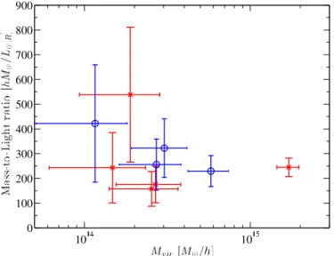
Method Rvir Mvir M(<500 kpch−1) κca Mvir/LRC χ2/dofb
(Mpch−1) (1015M
h−1) (1015M
h−1) (h M
/L) 1D WL+SLc 1.94±0.14 2.13+0.49
−0.44 0.63±0.17 <0.01 301±66 10/9
2D WLd 1.97±0.15 2.23+0−0..4438 0.54±0.12 0.03±0.01 310±57 25/7
X-ray 0.54+0−0..0408
SZE 0.50±0.04
Notes.
aThe constant dimensionless mass-sheet component. bThe goodness-of-fit, minimizedχ2over number of dof.
cThe NFW model was fitted to the mass profile fully reconstructed from WL+SL (see Section7.1), constrained by 1D
WL (shear+magnification)+SL Einstein-radius.
dThe NFW model was fitted to the mass profile reconstructed from WL alone (see Section7.2), using WL (2D shear+1D
magnification), without SL constraints.
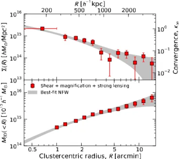
Figure 9.Top: surface mass density profileΣ(R) (squares) derived from a joint SL, WL distortion and magnification (WL+SL) likelihood analysis of ourHST+Subaru lensing observations. The gray area represents the best-fit NFW profile for the mass profile solutionΣ(R). Bottom: the cumulative mass
M2D(<R) (red squares) as derived from the full lensing analysis. The gray area
is the NFW fit (1σconfidence interval) to the WL+SL constraints as described above.
(A color version of this figure is available in the online journal.)
whereρsis the characteristic density, andrsis the characteristic
scale radius at which the logarithmic density slope is isothermal. The halo virial mass is then given by integrating the NFW profile (Equation (9)) out to the virial radiusrvir,Mvir≡M(<rvir). We
specify the projected NFW model with the halo virial mass, Mvir, and the degree of concentration,cvir ≡rvir/rs. We refer
all of our virial quantities to an overdensity ofΔc≡Δvir≈138
based on the spherical collapse model using the fitting formula by Kitayama & Suto (1996, their Appendix A).32
We constrain the model parameters p=(Mvir, cvir, κc) with our full-lensing mass profiles. Theχ2function for our SL+WL
32 Δvir≈140 using the fitting formula by Bryan & Norman (1998).
observations is33
χ2(p)= i,j
[si− ˆsi(p)]Cij−1[sj− ˆsj(p)], (10)
whereˆsiis the model prediction for the convergence profilesiat θiandCis the full covariance matrix ofsdefined asC=C+Clss,
withClssbeing the cosmic covariance matrix responsible for the
uncorrelated LSS projected along the line of sight. For details, see Umetsu et al. (2011b).
Our best-fit NFW model to the combined lensing constraints (Equation (10)) is shown in Figure9 as the gray shaded area. To summarize our results from this analysis, we obtain a total virial mass estimate ofMvir = (2.13+0−0..4944)×1015Mh−1 ∼
(3±0.6)×1015M
with the minimized χ2 of 10 for 9 dof (see a summary in Table5). We will compare and discuss all of the mass estimates yielded by the different modeling and reconstruction methods explored in the paper in Section9.1.
At larger radii, a flattening of the mass profile is observed, possibly indicative of the surrounding LSS. The deviation of the profile from a single spherical NFW halo at large radius is indicative of substructure associated with this cluster region, and therefore merits a more careful 2D analysis, which we present in the next sections.
7.2. Mass Profile Reconstruction Using Two-dimensional Shear and Magnification
We follow Umetsu et al. (2012) to extend the one-dimensional (1D) Bayesian method above (Section 7.1) into a 2D mass distribution by combining the spatial shear pattern (g1(θ), g2(θ))
with the azimuthally averaged magnification measurements nμ(θ) (Section 4.2), imposing a set of azimuthally integrated constraints on the underlying κ(θ) field.34 For details of the method, we refer the reader to Umetsu et al. (2012, their Appendix A.2).
By combining complementary WL distortion and magnifica-tion data in a non-parametric manner, we construct a 2D mass
33 The calibration uncertainties in observational parameters, such as the
background mean depths,β(back)(orzs,eff) andβ(red), have already been
marginalized over in the Bayesian mass profile reconstruction.
34 Since the degree of magnification is locally related toκ, this will essentially
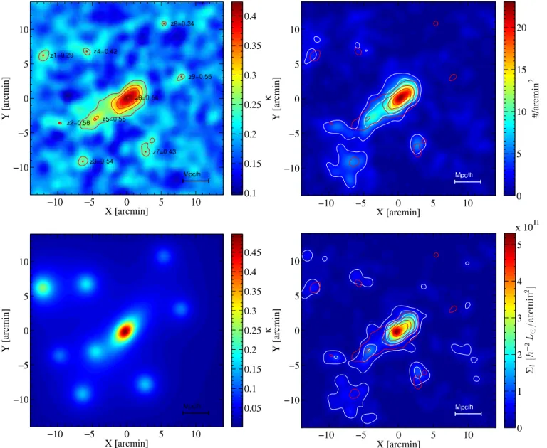
Figure 10.Top left: linear reconstruction of the dimensionless surface-mass density distribution, or the lensing convergenceκ(θ)=Σ(θ)/Σcrit, reconstructed from Subaru distortion data. The lowest red contour represents our detection level at 2.5σκ, with further increments of 2σκ. The red points denote the locations of the nine significant mass peaks identified above 2.5σκ. Top right: surface number density distributionΣn(θ) of green galaxies, representing cluster member galaxies. White contours show 5σnincrements starting at 2.5σn. Also overlaid are the red contours of the convergence, showing very good agreement between the DM and the galaxy distributions. Bottom left: dimensionless surface-mass density distribution reconstructed from the multi-halo shear-fitting analysis, comprising the NFW halos fitted to the nine main mass peaks detected in Figure10. The most massive central component was fitted by an elliptical-NFW model, whereas the other peaks are fitted by a simple NFW model. The parameters of each halo fit are given in Table5. Bottom right: luminosity density distributionΣl(θ) of green galaxies, representing cluster member galaxies. The white contours show 5σlincrements starting 2.5σlin number density. Also overlaid are the red contours of the convergence.
(A color version of this figure is available in the online journal.)
map over a 48×48 grid with 0.5 spacing covering the cen-tral 24×24field.35We show in Figure13(black circles) the azimuthally averaged radial mass profileΣ(R) produced from the resulting mass map, given in 10 linearly spaced radial bins spanning fromθ=1.5 to 16. The innermost bin with the hor-izontal bar represents the mean interior mass densityΣ(<1.5) as marked at the area-weighted centerθ=1. We find a model-independent constraint on the total enclosed mass withinθ≈7 to beM2D=(3.4±0.6)×1015Mh−1.
We fit an NFW + mass-sheet model (Equation (8)) to the WL radial mass profile derived here by minimizing the total χ2 function defined as in Equation (10), marginalizing over
35 The magnification analysis is limited within the central 24×24region
where the number counts of red background galaxies are reliably measured.
the mean background depth uncertainty in zs,eff. We find the
total virial mass to beMvir =(2.23+0.44
−0.38)×1015Mh−1. We
summarize all of the results from our analyses in Table5and discuss the differences in Section9.1.
8. SPATIAL MASS DISTRIBUTION ANALYSIS