Vol 9, No 1 (2017)

Implementation and Optimization of RWP Mobility

Model in WSNs Under TOSSIM Simulator

Lyamine Guezouli

, Kamel Barka

, Souheila Bouam

and Abdelmadjid Zidani

Computer Science Department, Lastic Laboratory, University of Batna 2, Batna 05078, Algeria

Abstract: Mobility has always represented a complicated phenomenon in the network routing process. This complexity is mainly facilitated in the way that ensures reliable connections for efficient orientation of data. Many years ago, different studies were initiated basing on routing protocols dedicated to static environments in order to adapt them to the mobile environment. In the present work, we have a different vision of mobility that has many advantages due to its 'mobile' principle. Indeed, instead of searching to prevent mobility and testing for example to immobilize momentarily a mobile environment to provide routing task, we will exploit this mobility to improve routing. Based on that, we carried out a set of works to achieve this objective.

For our first contribution, we found that the best way to make use of this mobility is to follow a mobility model. Many models have been proposed in the literature and employed as a data source in most studies. After a careful study, we focused on the Random Waypoint mobility model (RWP) in order to ensure routing in wireless networks. Our contribution involves a Random Waypoint model (in its basic version) that was achieved on the TOSSIM simulator, and it was considered as a platform for our second (and main) contribution, in which we suggested an approach based RWP where network nodes can collaborate and work together basing on our recommended algorithm. Such an approach offers many advantages to ensure routing in a dynamic environment. Finally, our contributions comprise innovative ideas for suggesting other solutions that will improve them.

Keywords: Mobility Model, Wireless Sensor Network, Random Waypoint, Routing.

1.

Introduction

In recent years, the technology of wireless networks has been growing thanks to technological developments in various areas related to microelectronics. In addition, with the emergence of Wireless Sensor Networks (WSNs), new themes have been opened and new challenges have emerged to meet the needs of individuals and the requirements of several areas application (industrial, cultural, environmental): observation of rare species life, monitoring of the infrastructure structure, optimization of treatment for patients, etc. These issues motivate many researchers. Indeed, despite the remarkable progress in this field, there are still many problems to solve. Thus, new protocols have been proposed to address the control of the medium access, routing, mobility etc. in sensor networks.

Regarding mobility, traditional Wireless Sensor Networks (WSNs) are developed using static nodes (SNs) [1]. These networks can be applied in numerous applications such as healthcare [2], military, industrial, monitoring, tracking based on multimedia sensor [3] and many other fields [4,5]. Hence, a lot of research and propositions are made for static scenarios. Nevertheless, the advanced technology involves applying more complex applications, which require mobility of its nodes. Mobility of nodes can enlarge WSN applications

[6]. Moreover, mobility can prolong the nodes lifetime, since data transfer between two nodes does not usually use the same relayed nodes in the path route. In addition, it serves to increase connectivity between nodes, since mobile nodes can help the communication between two isolated nodes [7]. It also helps to extend the coverage area of interest [8]. However, mobility can cause some challenging problems, like disconnection of nodes during the handover process. Other issues related to the nodes mobility are resource management, topology control, quality of services, security and routing protocol.

In a MWSN, there is at least one mobile entity and the remaining sensors are static. Mobile entities are able to communicate with neighboring sensors. In accordance with the role played, mobile entities can be either mobile base station, which acts as network data collector, or mobile sensors that detect changes in the environment or serve as data relay nodes. The mobility of the mobile SB patterns or mobile sensors could be used to improve network performance, such as the network lifetime. These mobile units can be introduced naturally or artificially placed. The mobility model of each mobile entity is generally determined according to the specific application and the size of the WSN.

In reality, mobility and deployment design of a MWSN is a complex problem that involves design requirements, mobility capability of mobile sensors, network environment, and application constraints such as time requirements. According to these design constraints, mobility strategy, collaborative model, the data packets and the routing protocol should be approached with caution in terms of network performance. The purpose of our work is divided into two objectives. Firstly we make the implementation of a mostly used mobility model by researchers (namely Random WayPoint mobility model - RWP) under one of the simulator dedicated to WSN (that is TOSSIM). That We Consider this implementation is paramount in the research field, as the RWP model is wide used among researchers (field of wireless networks). Secondly, We are interested to apply a variant of the mobility model RWP (named Routing-Random WayPoint "R-RWP") on the whole network in order to maximize the coverage radius of the Base Station (which will be fixed in our study) and thus to optimize the period the end-to-end delay for data delivery (this is to optimize Routing).

The paper is organized as follows:

represents the heart of our work. Afterwards, we continue with a presentation of different simulators dedicated to wireless sensor networks, then we introduce our contribution consists in introducing the RWP mobility model in TOSSIM simulator.

In the second part, we first present the works that are interested to optimize routing in mobile environment. Then, we present our contribution that consists of an update of RWP mobility model to optimize routing in such a mobile environment. We end with a presentation of the results obtained through simulation, and also a comparison with the basic RWP is presented.

This work will be completed with a conclusion and perspective.

2.

TOSSIM and mobility models

2.1. Related works

[9] analyze the performance of the mobility management scheme (i.e. PNEMO) with respect to RWP and CV mobility models. In order to implement an extensive simulation scenario as well as the modeling of the PNEMO scheme, new code is integrated with the current modules in NS 3 simulator environment. Simulation results show that the signaling requirements for these two models are much different. It is also indicated that the comparative handoff delay of PNEMO scheme may vary depending on different mobility model. [10]. have conducted detailed study of several entity and group mobility models that have been proposed in MANET research. Authors have proposed the new mobility model that covers some specific implementation area. Through simulations, Authors have found significant effect of attraction points in MANET performance. Because of attraction points, mobile nodes used to be accumulated in certain parts of simulation area forming small groups. Such accumulation around attraction point causes low packet delivery ratio compared to RWP mobility model. This result came because, nodes accumulate around attraction points, if source and destination node belongs in same cluster; delivering packets from source to destination does not take long time. If source and destination belongs to different cluster, packet gets lost or remains in buffer of some neighboring nodes.

[11] studied the connectivity of the network of MANETs considering Random Waypoint Mobility model by changing number of nodes, simulation time, length and width of the simulation area. Authors also studied the connectivity if agent nodes are used. They give an approximate idea of minimum number of nodes required to be deployed to achieve network connectivity of particular area if Random Waypoint Mobility model is considered. Authors also show the usefulness of agent nodes to improve connectivity if Random Waypoint Mobility pattern of the nodes are considered.

2.2. Mobility models

Mobility is an important factor in wireless networks. It represents the movement of mobile nodes (MNs) and how their speed and direction are changed over time. Mobility models represent or predict user's or wireless device’s movements. These models are often used to simulate or emulate the actual movement of the devices in terms of

geometry, speed, etc., in a geographic area. A significant body of literature [10] has shown that the mobility directly affects communication performance in terms of throughput and delay. Mobility models can be simulated in two ways: using traces obtained through real experiments, or generating synthetic data using the statistical characteristics. Traces are real mobility patterns that exist in life. Synthetic is trying to realistically represent the movement of users in the absence of traces availability. There are many different ways to classify synthetic mobility models such as individual and group mobility models “as shown in Table 1”.

Table 1. Classification of mobility models Mobility models

Group Mobility Models Individual Mobility Models Nomadic [12] Random Walk [13]

Column [13-12] Random WayPoint [14] Exponential Correlated

Random [15] Probabilistic Random Walk [13] Pursue [12] Random Direction [13] Reference Point [16] Gauss – Markov [17]

• Individual models, where the mobility of each node are determined independently of each other.

• Group models, which take into account the correlation of movements between some nodes. These models divide the nodes into several groups and end up a relationship between the mobile units belonging to the same group. In addition, there are three types of law of movement: random, deterministic and hybrid

• Random patterns are random arbitrary displacement and without environmental constraints. These are simple models to implement and therefore widely used.

• Deterministic models, are based on traces (behaviors of users observed in actual systems).

• Hybrid models achieve a compromise between simplicity and realism, but are difficult to implement.

Among the individual models, we can cite: Random Waypoint, Random Direction, and Gauss-Markov. RPGM (Reference Point Group Model) and Sanchez models are the most used group mobility models. The Manhattan models (representing the movement of nodes in an urban area) and Freeway (modeling the movements of vehicles on a road network) are hybrid models based on the use of maps. We will describe more precisely in what follows the Random Waypoint model, the model on which we will base our study.

2.3. Random Waypoint Model

This model was first used by Johnson and Maltz in the evaluation of the routing protocol DSR [18] and was then refined by the same authors. The Random Waypoint is used to model all scenarios in which the nodes move toward a destination, take a pause time at arrival, then move to another destination, and so on. In this model each node chooses randomly, as a destination point of coordinates (x, y) in the surface of simulation, and a speed between 0 and Vmax. The node trips to the chosen destination with the selected speed. Upon arrival, the node takes a pause time before to again choose a new destination and a new speed to repeat the same process. Studies have been made on this model since it is the model most often used in the simulations due to the ease of its implementation. Some studies have treated the initialization of this model and the convergence time of simulations in the case where the nodes begin by taking a pause time. In [19], it is shown that the Random Waypoint, in its current form, does not reach a state of equilibrium, but rather that the speed is decreased without interruption while the simulation progresses, which can distort the results. Based on the carried out analyzes, the authors propose a simple solution which is to choose a strictly positive value for the minimum speed.

Figure 1 shows example traveling pattern of a mobile node using the random waypoint mobility model starting at a randomly chosen point or position (133, 180); the speed of the mobile node in the figure is uniformly chosen between 0 and 10 m/s [13].We note that the movement pattern of a mobile node using the random waypoint mobility model is similar to the random walk mobility model [13] if pause time is zero. In most of the performance investigations that use the random waypoint mobility model, the mobile nodes are initially distributed randomly around the simulation area. This initial random distribution of mobile nodes is not representative of the manner in which nodes distribute themselves when moving.

Random Waypoint applied for each mobile p the following instructions:

do {

Step 1: Select a new value for DestP uniformly in each direction.

Step 2: Select a new value for Vp uniformly on the interval [Vmin, Vmax].

Step 3: Move it mobile p to DestP with speed Vp; Step 4: Select a new value for PauseP uniformly on

the interval [Pmin, Pmax]. Step 5: Pauses a PauseP duration; }

While (end of simulation time) Such as:

• DestP : Cartesian coordinates of the point towards which the mobile p.

• Vp : speed mobile p defined on the interval [Vmin, Vmax].

• PauseP : mobile p pause time defined on the interval [Pmin, Pmax].

2.4. Wireless Sensor Network Sımulators

Sensor network simulators are many and varied. This makes choosing the best very difficult simulator for a generic application. Indeed, each is differentiated by other characteristics that make him the best for a very specific application, under defined conditions. However, the same simulator may be not the good simulator in other circumstances or for other applications.

• Ns (network simulaton) (also known as the ns-2) is a network of discrete event simulator. It is popular in the research community by its extensible nature, nature as free software and the availability of a rich documentation on the internet. This simulator is instead used for the simulation of routing protocols and emission / reception and especially for research in the ad-hoc networks. • OPNET (Optimum Performance Network) is a network

simulation tool very powerful and very complete. OPNET is based on an intuitive graphical interface; the use and mastery are relatively easy. In fact, it has three levels: the network domain, the node domain and process domain. This is a simulator of WSN, object oriented, written in C and C ++ with a very rich library but it is not available to everyone. In fact, OPNET is only available under a commercial license.

• OMNeT ++ is a discrete event simulator. It is based on a component-oriented architecture, the modules are written in C ++. OMNeT was primarily designed to simulate the communication in networks but thanks to its flexible architecture and generic, it was then used for many other applications. Although OMNeT is not a network simulator itself, it is gaining wide popularity as a network simulation platform to the scientific community and the industrial area.

• TOSSIM is the TinyOS simulator. Indeed, this is a simulator / emulator discrete event sensor networks equipped with the TinyOS operating system. It is disseminated by the availability of its code and its nature as free software. TOSSIM can run on Linux or Windows. Its great advantage over many other sensor networks simulators is that it supports different types of nodes in WSN. Indeed, TOSSIM can simulate the operation of mica, imote, MICA2, MICA2-dot, micaz, telos telos-HC08, telosa, telosb and tmote. In addition, it can simulate a very large number of nodes in a single simulation. Simulations with TOSSIM give us an idea about the functioning of the network, the transmission / reception, the radio links between nodes, error messages, etc.

Table 2: Overview of simulators characteristics dedicated to WSNs

2.5. Implementation of mobility within RWP model into TOSSIM

In this section, we will detail the main steps to implement the RWP mobility model in Tossim and this using two programming languages Java and Python, simulation thereafter be made with the Tossim simulator.

In TOSSIM simulator, each node is represented by the MOTE.java class, which is an extension of the SimObject.java class.

To provide mobility to the nodes, we have to add a new function (called mobilitymodel(X,Y,Z,S) ) in the main class SimObject.Java.

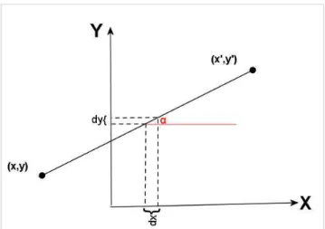
This function moves a given node from a position (X, Y, Z) to the destination (X ', Y', Z '), this movement will be based on a predetermined speed S as shown below.

However, in order to reach the destination (x ', y', z '), the node has to travel a distance (As shown in Error! Reference source not found.)

Figure 2: Representation of a node displacement from a position (x, y, z) to a destination (x', y', z')

(1) This distance is represented by a set of steps, the cardinal of this set (Nsteps) is calculated by the function CalcNSteps(de) according to the distance .

Each step must be performed in a dt time, such as:

⇒

⇒

Thereafter, we continue our work with a 2D plane, the third axis Z will be practically the same results as those of X and Y (As shown in Error! Reference source not found.).

Figure 3: Representation of a node displacement from a position (x, y) to a destination (x', y') with angle. In order that the node reaches the destination, the node jumps step by step. To jump one step, the node will update its current coordinates (Xt, Yt), this update is the representation of a projection of a step by the axes x, y as following:

(3) (4) At the first, Xt, Yt have initially the position X, Y respectively.

When the node arrives at its destination, we can conclude that he had traveled (along each axis) as follows:

(5) (6) Since the travel time by one step (dt) is really restricted (become zero), the equations mentioned above become as follows:

(7) (8) Such as: ts is the time simulation at the current position. Now, to better optimize our functions, we need to calculate the cos and sin

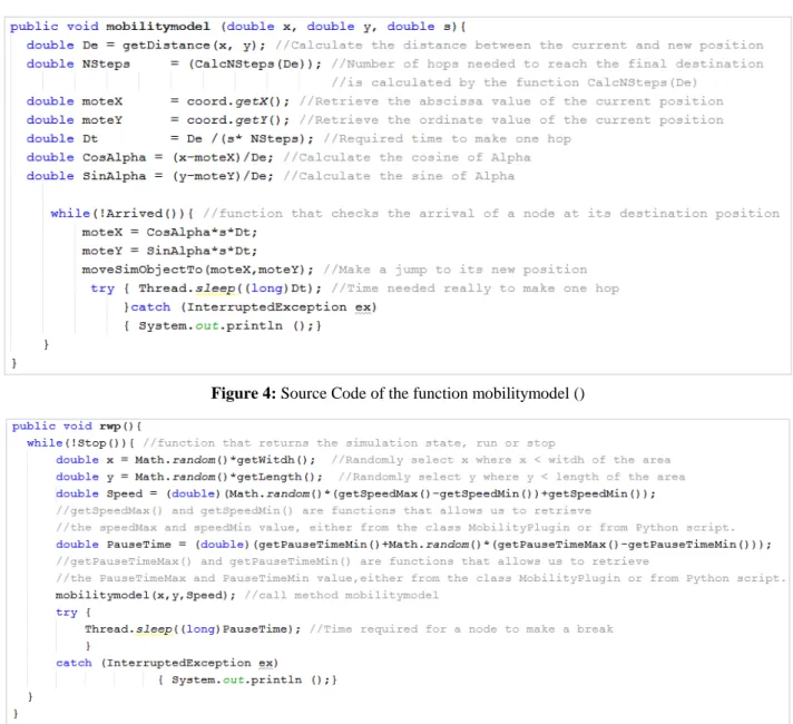
(9) (10) As conclusion, we proceeded to programming a function to include all these equations, and to ensure the mobility of a node, we must make a simple call to this function named mobilitymodel (X, Y, S) with parameters: Coordinates to the new position and Speed.

Hereinafter, the source code of the function mobilitymodel(X,Y,S).

This function represented in Error! Reference source not found. is able to be used to set any mobility model to simulate the movement of nodes in a network.

However, to ensure mobility based on RWP model, we used a new method (named RWP()) in SimObject.java class.

Architecture Standard Extension for

Consumption

Ns-2 Oriented Object 802.11,

Bluetooth…

No

OPNET Oriented Object 802.11,

802.16, mobile IP

No

OMNeT oriented component 802.11 No

Figure 4: Source Code of the function mobilitymodel ()

Figure 5: Source Code of the method rwp ()

This method determines for each node N (were selected in a random manner):

• its new position (X', Y') included in the simulation area, • its speed ‘S’ in the interval [SpeedLow - SpeedHeight], • its pause time ‘Time’ in the interval [PauseTimeMin,

PauseTimeMax].

Obviously, this method will call the function mobilitymodel(X,Y,S) as with parameters the first two defined above (i.e. position (X', Y') and S). Once at the desired position, node N will mark a pause time ‘Time’. The process will be repeated for each cycle until the end of the simulation.

The source code of the method rwp() is represented in Error! Reference source not found..

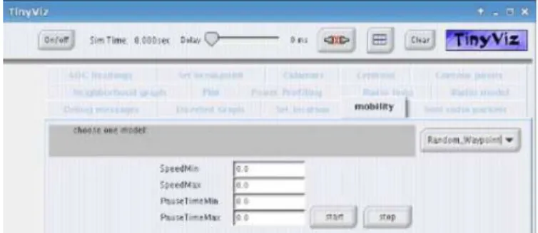
To view the movement of the nodes constituting the network in the simulation area, and to determine the appropriate parameters and to choose the appropriate mobility model, we implement in TinyViz a new interface (new plugin) called 'Mobility'.

However, to execute the simulation, we had to choose between a silent execution with a simple python script, or using the plugin 'Mobility' in TinyViz.

• With Python: In this type of execution, we will not see any visual representation of nodes in the network. We created a script mobility.py where we called the method RWP() for each node with class mote. We created this method in the package sim.script.reflect.*.

• With TyniViz: A plugin must be a subclass of net.tinyos.sim.Plugin. As a first step, we added a subclass MobilityPlugin.java

This subclass displays an interface allowing the user to choose the mobility model among many, then to enter the settings for the selected model (in our study, we were only interested by the RWP model):

o4 TextField as respectively: SpeedLow, SpeedHeight, PauseTimeMin, PauseTimeMax.

o2 Buttons: Start, which allows to start the simulation, and the stop button that stops the simulation.

To start the simulation by the Start button, we will launch the RWP model for each node in the simulation area.

Figure 6: The mobility plugin subclass interface.

2.6. Simulation results

There are mobility metrics which can be used to observe the mobility policies. Relative velocity, maximum velocity, acceleration, pause time are some examples. Those metrics can be observed for different mobility models and can conclude some facts regarding the mobility characteristic of those models. Varying those characteristics, we can draw how much those metrics are important for a protocol operation. For our study, we use the following metrics as evaluation metric to test the performance of our proposed mobility model (R-RWP proposed in the next part) compared to the mobility model (RWP).

• Packet delivery ratio : Packet delivery ratio counts the number of packets originated by the source and number of packets received by the receiver. During communication, nodes move from its position continuously with different velocity. We can compare the ratio of packets send by sender and received by receiver to evaluate the effect of our changes parameter of mobility over the performance of network.

• Average end to end delay : Packet delay is time that packet takes from source node to destination. In MANET, packet relays from several intermediate nodes. So, delay of a path is summation of all the links along that path. Link fluctuates during the mobility of nodes. Some links along path may have high delay comparing to others. Average value gives the value that can be compared with other results. Average packet delay increases with mobility in MANET.

The simulation results will be presented and discussed in the second part to make the necessary comparisons.

3.

R-RWP - A variant of RWP to improve

routing in WSNs

3.1. Related works

In the literature, there are two categories among the methods for routing in mobile networks. The first concerns the methods where sensors based their arguments on the positions of their one or two hops neighbors. The second is composed of methods which define a geographic region and disseminate to the interior of this region a message to reach the destination. These two categories will focus respectively the names neighborhood-based routing and region-based routing.

For Neighborhood-based routing, methods in this category are mostly adaptations of routing methods for static networks. They assume that the displacement sensor

maintains the same distribution in the deployment area than that present in the case where the network is static. Thus, all the methods described above for static networks can be adapted to the context of mobility. The major disadvantage of these routing techniques is that the sensors must always ask the positions of their neighbors to one or two hops to send a message. Specifically, when a sensor needs to send a message to a destination, it sends a first message to request the positions of its neighbors (the operation is repeated by each of the neighbors, when knowledge of the positions of two-hop neighbors is required). After the response of neighbors, the sensor selects the next relay node and makes him follow the message. It is preferable, considering mobile sensors to avoid such message exchanges.

However, for the Region-based routing category, the sensors need to know just their own position and the position of the destination. When a source wants to send a message to a destination, it defines a geographic region containing its position and that of the destination and he sends his message through this region to reach the destination. The methods [20,21,22,23] are examples of this. The geographic areas may take different forms: for example, in [21] the region used is a rectangle, whereas in [23] is the case of an ellipse. Once the region is defined, the source sends its message and when a sensor receives it, it tests depending on its position if it belongs to the region and, if appropriate, forwards the message. In order to consume as little energy as possible, it is for these methods to define the smallest possible area or select a subset of relay nodes within the region. This is the author’s work, for example, in [22,23].

It should be noted again that all of these methods assume that the sensors know their positions and, if necessary, their neighbors with accuracy.

The technique of routing in mobile sensor networks which is proposed in the following of this paper will essentially make possible to lighten the operation of routing in the network regardless of the positions of nodes. Indeed, it is a solution based on a mobility model, the mobility of sensor nodes is a very influential factor in this type of networks. We try through this work to exploit the benefits of this mobility. In the following sections, we give a brief description of mobility models, we expose the RWP model and expose our algorithm of the proposed approach, and we end up with simulation results.

3.2. Performance of the Routing Protocols with the Mobility Models

In [24] the authors presents an accurate evaluation of the impact of the mobility models on the performance of routing protocols, this evaluation requires testing multiple mobility patterns and different routing protocols. Otherwise, the observations made and the conclusions drawn from the simulation studies may be misleading.

Table 3: Ranking of routing protocols PDR (%) over different mobility models [24].

Model

Protocol

RWP EGM ST GM RD

Flooding 99.2 98.2 96.8 98.2 96

RGP 92 90 88 86 83

AODV 78 74 72 75 73

OLSR 76 69 65 68 61

In our study, we will consider these results to the choice of routing protocol used in our approach. We can deduce that in the case of a mobile environment, flooding presents the most interesting routing protocol in such cases. Also, in conjunction with the flooding, the mobility model that seems interesting is the RWP, hence our choice for such a model. 3.3. Algorithm of the proposed R-RWP model

We propose in this work a new way to route the information collected from mobile sensors nodes, without necessarily having to use or modify a robust routing protocol for such an operation. The principle of our method is based on a mobility model.

Indeed, the mobile sensor nodes must follow a mobility model to move in the environment. Our method is an optimization of the RWP model to generate a new model: R-RWP (Routing - Random WayPoint) able to route information in a mobile environment.

The algorithm of our R-RWP model is as follows:

The nodes move freely in the environment (depending on model RWP).

During his pause time, each node Y which has information for BS (high % of information in the memory of the node), updates its one hop neighbor table (Vy) and verify:

If BS ∈ Vy

TPy = ∞ (The node Y is stabilized to ensure

communication with the BS)

If Memroy of Y is not empty

(Y sending data to the BS and frees its

memory)

For each Xi (Xi ≠ BS & TPXi ≠∞) direct neighbor of Y:

(Y informs its neighbors that it has a direct

link with BS)

If the Xi is interested by the BS (Memory of Xi is not

empty):

∥ TPXi = ∞

TPXi = 0

TPy = 0

3.4. Simulation and results

We use TOSSIM [25,26] for simulating our approach. TOSSIM is a discrete event simulator for TinyOS sensor networks.

TinyOS [26] is a system developed and supported primarily by the American University of Berkeley, which offers the download under the BSD license. Thus, all sources are available for numerous hardware targets.

TinyOS is an open-source operating system designed for Wireless Sensor Networks. It respects an architecture based on a combination of components, reducing code size required for its implementation. This is in compliance with the constraints observed by sensor networks memories.

TOSSIM’s primary goal is to provide a high fidelity simulation of TinyOS applications. For this reason, it focuses on simulating TinyOS and its execution, rather than simulating the real world. While TOSSIM can be used to understand the causes of behavior observed in the real world, it does not capture all of them, and should not be used for absolute evaluations.

We compared the performance of our approach (R-RWP) with the one based on RWP in its basic version.

About metrics for routing, we based our simulations on two scenarios: The first scenario will be used to measure the performance of our proposal in terms of transmitted messages and a second one will measure the latency for the delivered data.

Also, for the metrics concerning mobility, two scenarios will be discussed, one that calculates the number of neighborhood, in an amount of time, for a station that has a direct link with the BS. For the second scenario, we try to find out the number of active links between the BS and its neighbors.

3.4.1 Parameters used in the simulation scenarios

First of all, we assume that the environment is without any obstacles during the entire duration of simulation.

environment), and will be disabled during the startup phase (the first Fifteen minutes) to allow time for the sensors to capture data. Network’s links packet loss rate probability is 5%, the duty cycle of each node is fixed at five minutes and the sleep period for each node is zero minute. For mobility pattern, each node moves according to the random waypoint mobility model (RWP) such as the minimum and maximum speeds are 0,05m/s and 0.3m/s, respectively. These simulations were run during one hour. It should be noted that the pause time used in our various scenarios is fixed for a period of five seconds. To optimize the energy of the network, each mobile sensor node will have its radio switched on during each pause marked by this sensor.

Figure 7: Initial dispersion of nodes in the environment Each scenario has been played 100 times taking into account the period of heating and cooling of the network, the collection of results only starts after 900s of simulation (time required to begin capturing information from the environment) and stops 300s before the end of the simulation.

Table 4 summarizes the parameters used.

Table 4: Parameter values used in simulations

Parameters Values

Observation area 100 m × 100 m Nodes number 100

Base station position (50,50) Communication range 16 m

Packet data max size 10 bytes Memory space size 100 bytes Packet loss rate on each link 5%

Min speed 0.05 m/s Max speed 0.3 m/s Sleep period 0 min

Duty cycle 5 min Simulation time 1 hour 3.4.2 Simulation results

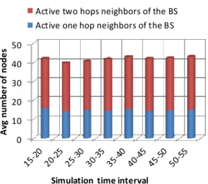
Figure 8 represents the sum of one and two hops neighbors of BS. These results are grouped to better perform the necessary comparisons.

It appears that based on the metric relating to the number of nodes in the BS Neighborhood, we find, generally, a significant number of nodes which is the effect of using RWP.

Figure 8: Number of neighbors with BS (one hop)

We can notice that the number of active nodes is almost identical to the number of one hop neighbors, especially in the beginning of the simulation. This happens because every node has to transmit a datum to the BS during a specific cycle and can be noticed at the beginning of the simulation where a time startup of 15 minutes is leaved before transmitting captured data to the BS. This period allows collecting an important amount of data in sensor nodes caches (3 messages in every node’s cache).

The simply difference that we can notice between the two histograms is due to the packet loss rate (the probability that a node can lose packets) that we specified in the simulation parameters. The end of the simulation shows that there is a little increase in the histograms difference which is a logical result because the network becomes gradually lighter in terms of sensor nodes caches memories.

Now back to reveal the results obtained for the two-hops neighbors. The Error! Reference source not found. shows the results.

0 20

A

v

g

N

u

m

b

e

r

o

f

n

o

d

e

s

Simulation time interval Active two hops neighbors of the BS

Two hops neighbors of the BS

The two hops neighborhood seems to be more important compared to the one hop one. This can be explained by the fact that a two hops neighbor node can be himself a neighbor to multiple one hop nodes during the whole period of a determined cycle (fixed to 5 minutes in our simulations). About the difference between active neighbors and non-active ones, the interpretation is the same as for the earlier figure concerning the one hop neighborhood.

Indeed, the number of two-hops neighborhood seems important, hence the necessity to exploit the situation to transit as soon as the data captured by the mobile sensors. After all these results, we can deduce an interesting large number of two hops neighborhood of BS, it will exploit it to ensure optimal routing in delays mainly realistic.

Thereafter, we are studying the routing-related metrics to test the reliability of the routing side in our approach.

Formally, we are interested in finding the probability that a mobile sensor node will be neighbor (direct or 2-hops) with the base station during a time interval.

0 10 20 30 40 50

A

v

g

n

u

m

b

e

r

o

f

n

o

d

e

s

Simulation time interval

Active two hops neighbors of the BS Active one hop neighbors of the BS

Figure 10: Neighborhood of the BS with R-RWP

However, as it appears in Figure 10, we can deduce that the probability that a node will be able to be in contact with the BS increases with our R-RWP solution, since our solution extends the BS coverage area by exploiting the two-hop neighbors.

Now, as the essential aim of any routing process is to deliver the data, and referred to simulation results we obtained, we made extraction results related to the number of messages received by the BS.

Figure 11 is a presentation of the results obtained after the simulation time.

Figure 11: Number of messages received by the BS with RWP & R-RWP

With RWP model, the delivery rate is less significant than with R-RWP for the simple reason that with the R-RWP, the BS communicates with one and two hops neighbors. But with RWP, the BS communicates only with one hop neighbors. Thus, with R-RWP the number of messages received by the BS will increase rapidly, which will certainly influence on the buffers occupancy rate of the mobile sensor nodes. Now, we'll look at the end-to-end delay that will have to wait a packet to reach the BS.

Error! Reference source not found. shows the simulation results.

Figure 12: Latency average with RWP & R-RWP

As we can see, the packets in RWP take a long time to communicate with BS. Indeed, this is the consequence that to begin the exchanging with the BS, a mobile node does not transmit its data to any other node, and keep its data until it detects the BS in its coverage area, from which time the exchange will begin.

However, with R-RWP the discovery of the BS will occur at the coverage area of the node of in question, and also at the coverage area of the neighboring nodes of the node in question. This strategy provide us a considerable gain in the end to end delay, this is a result of collaboration between the mobile nodes.

3.5. Discussion

Regarding energy consumption, it is certainly clear that there's a proportional relationship between the exploitation of intermediate nodes (for routing information) and energy consumption.

The more the number of intermediate nodes in the network is important, the more the dissipation of energy will be significant. In our approach we have exploited more than 10% of nodes with the model RWP.

However, we have filled this degradation by a strategy of activation of radio antennas. However, in case of mobility, and to avoid interrupting communications, we have chosen to turn off the radio of wireless sensor nodes until they reach their pause time. During this pause time the mobile sensor looks for the BS to forward the concerned data.

4.

Conclusion and Future Work

In this work we proposed First of all an implementation of the RWP mobility model under TOSSIM simulator, hence the use of such model under this type of simulator will be just a manipulation case under TOSSIM interface.

After that, we designed a new routing method which is aware of mobility, and then we carried out a study that aims to test the performance of our approach in a mobile sensor environment. It should be remembered that our objective is to exploit the mobility of nodes to alleviate routing in such networks, especially because of large issues that can be raised during designing suitable routing protocols for such environment.

Thereafter, and as perspectives for this work, we plan to first compare the results with those performed on the basis of routing protocol dedicated for mobile sensor networks. Then we propose to study the behavior of our approach in an environment with obstacles. The study is in process; its principal is to find the ideal position for the BS.

References

[1] J. Yick, B. Mukherjee, and D. Ghosal, "Wireless sensor network survey," Computer Networks: The International Journal of Computer and Telecommunications Networking, vol. 52, no. 12, pp. 2292-2330, 2008.

[2] Stanković _{and Stanislava, "Medical Applications of} Wireless Networks," Transactions Journal on Internet Research, vol. 5, no. 2, pp. 9-23, July 2009.

[3] I. Boulanouar, A. Rachedi, S. Lohier, and G. Roussel, "Energy-aware object tracking algorithm using heterogeneous wireless sensor networks," 4th. IFIP/IEEE Wireless Days 2011, pp. 1 - 6, October 2011.

[4] S. Prasanna and S. Rao, "An Overview of Wireless Sensor Networks Applications and Security," International Journal of Soft Computing and Engineering (IJSCE), vol. 2, no. 2, May 2012.

[5] J. A. Stankovic, A. D. Wood, and T. He, "Realistic Applications for Wireless Sensor Networks," in Theoretical Aspects of Distributed Computing in Sensor Networks, 14312654th ed.: Springer, 2011, pp. 835-863.

[6] L. M. L. Oliveira, A. F. de Sousa, and J. J. P. C. Rodrigues, "Routing and mobility approaches in IPv6 over LoWPAN mesh networks," International Journal of Communication Systems, vol. 24, no. 11, pp. 1445-1466, November 2011.

[7] A. Ghosha and S. K. Das, "Coverage and connectivity issues in wireless sensor networks: A survey," Journal of Pervasive and Mobile Computing, vol. 4, no. 3, pp. 303–334, 2008.

[8] B. Liu, P. Brass, O. Dousse, P. Nain, and D. Towsley, "Mobility improves coverage of sensor networks," MobiHoc '05 Proceedings of the 6th ACM international symposium on Mobile ad hoc networking and computing, pp. 300-308, 2005.

[9] S. Islam, A. A. Hashim, M. Hadi Habaebi, S. A. Latif, and M. K. Hasan, "A simulation analysis of mobility

models for network mobility environments," ARPN Journal of Engineering and Applied Sciences, vol. 10, no. 21, 2015.

[10] S. Raj Bhandari, G. M. Lee, and N. Crespi, "Mobility Model for User's Realistic Behavior in Mobile Ad Hoc Network," Communication Networks and Services Research Conference (CNSR), 2010 Eighth Annual, pp. 102 - 107, May 2010.

[11] A. Pramanik, B. Choudhury, T. S. Choudhury, and W. Arif, "Simulative study of random waypoint mobility model for mobile ad hoc networks," Communication Technologies (GCCT), 2015 Global Conference on, April 2015.

[12] W. Chen and P. Chen, "Group mobility management in wireless ad hoc networks," Vehicular Technology Conference, 2003. VTC 2003-Fall. 2003 IEEE 58th, vol. 4, pp. 2202 - 2206, October 2003.

[13] T. Camp, J. Boleng, and V. Davies, "A Survey of Mobility Models for Ad Hoc Network Research," Wireless Communications for Mobile Computing (WCMC) : Special issue on Mobile Ad Hoc Networking : Research, Trends and Applications., vol. 2, no. 5, pp. 483-502, 2002.

[14] C. Bettstetter, H. Hartenstein, and X. Pérez-Costa, "Stochastic Properties of the Random Waypoint Mobility Model," Journal of Wireless Networks, vol. 10, no. 5, pp. 555 - 567, September 2004.

[15] M. Bergamo et al., "System design specification for mobile multimedia wireless network(MMWN)," Technical report, DARPA project DAAB07-95-C-D156, 1996.

[16] X. Hong, M. Gerla, G. Pei, and C. Chiang, "A Group Mobility Model for Ad-Hoc Wireless Networks," MSWiM '99 Proceedings of the 2nd ACM international workshop on Modeling, analysis and simulation of wireless and mobile systems, pp. 53-60, 1999.

[17] B. Liang and Z. J. Haas, "Predictive distance-based mobility management for multidimensional PCS networks," IEEE/ACM Transactions on Networking (TON), vol. 3, pp. 718-732, October 2003.

[18] D. B. Johnson, D. A. Maltz, and Y. Hu, "The Dynamic Source Routing Protocol for Mobile Ad Hoc Networks (DSR)," IETF MANET Working Group - INTERNET-DRAFT, July 2004.

[19] J. Yoon, M. Liu, and B. Noble, "Random waypoint considered harmful," INFOCOM 2003. Twenty-Second Annual Joint Conference of the IEEE Computer and Communications. IEEE Societies, vol. 2, pp. 1312 - 1321, April 2003.

[20] D. B. Johnson and D. A. Maltz, "Dynamic source routing in ad hoc wireless Networks," in Mobile Computing, Springer US, Ed. USA: Kluwer Academic Publishers, 1996, vol. 353, ch. 5, pp. 153-181.

[21] Y. Ko and N. H. Vaidya, "Location-aided routing (lar) in mobile ad hoc networks.," Wireless Networks , vol. 6, no. 4, 2000.

(TON), vol. 14, no. 3, pp. 479-491, 2006.

[23] X. Li, K. Moaveninejad, and O. Frieder, "Regional gossip routing for wireless," Mobile Networks and Applications, vol. 10, no. 1-2, pp. 61–77, 2005.

[24] J. Madjo, T. Kunz, Y. Zhou, M. St-Hilaire, and M. Biomo, "Unmanned Aerial ad Hoc Networks: Simulation-Based Evaluation of Entity Mobility Models’ Impact on Routing Performance," Special Issue Unmanned Aerial Systems, pp. 392-422, 2015.

[25] P. Levis, N. Lee, M. Welsh, and D. Culler, "TOSSIM: accurate and scalable simulation of entire TinyOS applications," SenSys '03 Proceedings of the 1st international conference on Embedded networked sensor systems, pp. 126-137, 2003.

[26] J. Li and G. Serpen, "Simulating Heterogeneous and Larger-Scale Wireless Sensor Networks with TOSSIM TinyOS Emulator," Conference Organized by Missouri University of Science and Technology - Washington D.C., vol. 12, pp. 374-379, 2012.

[27] I. Aloui, O. Kazar, L. Kahloul, S. Servigne, "A new Itinerary Planning Approach Among Multiple Mobile Agents in Wireless Sensor Networks (WSN) to Reduce Energy Consumption" International Journal Of Communication Networks And Information Security (IJCNIS), Vol. 7, No. 2, pp. 116-122, August 2015. [28] A. A. El Arbi, S. Alaoui,, H. Moha and Y. Qaraai,