Traf
fi
c-Flow Analysis for Fast
Performance Estimation of
Communication Systems
G´abor Lencse
Department of Telecommunications, Sz´echenyi Istv´an University of Applied Sciences, Gy¨or, Hungary
The traffic-flow analysis(TFA) is a promising method
for the performance estimation of communication sys-tems. TFA produces approximate results with much less computation (that is, much faster) than discrete-event
simulation of the system.
In the first step, TFA distributes the traffic in units of properly chosen size using the actual routing algorithm of the network. In the second step, TFA adjusts the time distribution of the traffic according to the finite capacities of the network.
It was found that the results of TFA approximate the results of the analytical method well.
Keywords: communication networks, performance anal-ysis, traffic modelling, discrete-event simulation, impor-tance sampling
1. Introduction
Simulation is a widely used method for the per-formance analysis(Jain, 1991)of
communica-tion systems. There is a large number of vari-ous methods used to describe the behaviour of complex systems. (Banks et al., 1996;
Brat-ley et al., 1986; J´avor, 1985; J´avor, 1993)The
simulation of large and complex systems re-quires a large amount of memory and comput-ing power that is often available only on a su-percomputer. Efforts are made to use multipro-cessor systems or clusters of workstations. The conventional synchronisation methods for par-allel simulation(e.g., conservative, optimistic)
(Fujimoto, 1990) use event-by-event
synchro-nisation and they are unfortunately not applica-ble to all cases, or do not provide the desiraapplica-ble speedup. The conservative method is efficient only if certain strict conditions are met. The
most popular optimistic method “Time Warp”
(Jefferson et al., 1987) often produces
exces-sive rollbacks and inter-processor communica-tion. The Statistical Synchronisation Method proposed by Pongor (Pongor, 1992) does not
exchange individual messages between the seg-ments but rather the statistical characteristics of the message flow. The method can produce excellent speed-up (Lencse, 1998a) but has a
limited area of application(Lencse, 1999).
made. Thetraffic-flow analysis(TFA)can
ful-fil this need. TFA is a combination of simulation and analytical and/or numerical methods.
Un-like detailed simulation, TFA does not distribute the traffic in the network packet by packet but in larger units of carefully chosen size. TFA determines the time distribution of the traffic separate from the spatial distribution. The com-putational cost of the whole procedure — and in this way the execution time too — may be much less than that of the detailed simulation of the system.
This paper is organized as follows: first, a gen-eral description of TFA is given, then the se-lected traffic model is depicted including its op-erations, next some critical questions are dis-cussed, afterwards an implementation of the method is shown, finally a case study is given: TFA is compared with the pure analytical me-thod.
This topic was identified as being of importance in the fast performance analysis of large com-munication systems.
2. General Description of the Method
2.1. The Networking Model of the Traffi c-Flow Analysis
The traffic-flow analysis assumes that the model of the network is built up by nodes (routers,
switches, etc.) and transmission lines. The
traffic of the network is generated by applica-tion modelsconnected to the nodes. The inten-sity and the time distribution of the traffic are described by a mathematical model (typically
statistics).
TFA is a general method which can work with various traffic models and routing algorithms. The requirements for the traffic model will be given after the basic description of the operation of TFA.
2.2. The Operation of the Method
A program which does traffic-flow analysis on the model of a network produces results in two phases.
Phase 1. — Determining the spatial distribution of the traffic
In the first phase, the applications in the model send the generated traffic to their destinations inrouting unitsof parametrised size. (Routing
units are the basic portions of the traffic that are handled together.) The nodes forward the
routing units according to the routing algorithm of the modelled network while the lines and the nodes record the characteristics of the traffic flowing through them. The nodes may use the line capacity values for the routing decisions, but the time distribution of the traffic is not in-fluenced by the finite capacities of the lines and nodes in this phase. The time distributions of the traffic transferred on various elements of the network are stored at the elements and will be summed up in the second phase according to the method described there.
Phase 2. —- Determining the time distribution of the traffic
In the second phase, we must sum up the trans-ferred traffic for the lines and nodes. The ad-dition uses the adad-dition operation of the traffic model. The operands are summed up first and the finite capacity is only taken into consider-ation at the end. This method will be detailed when discussing the selected traffic model.
2.3. Requirements for the Traffic Model
The traffic model must fulfil the following re-quirements:
It is possible to describe the intensity and time distribution of the traffic by a mathe-matical model called thetraffic model. The traffic model is closed for the operation of addition: that is, the summed up traffic will be characterised with the same methods as its components.
It is possible to calculate the effect of the finite capacities of the nodes and lines to the time distribution of the traffic. (The
traf-fic model is not necessarily closed for this calculation.)
conference, web, etc.) can be handled
to-gether or even in units of arbitrary size, as aggregated traffic model.
The traffic of all the source and destination node pairs can be handled in arbitrary order.
2.4. What are the Capabilities of the Traffi c-Flow Analysis?
TFA is able to determine some classic statisti-cal characteristics of the traffic on the nodes and lines of the network such as throughput, delay, etc.
TFA tells us the steady state behaviour of the network.
The application models handle together the traf-fic of several applications, that even alone may consist of large number of sent/received
pack-ets. As TFA takes statistics through the net-work, they do not need to be collected on the basis of a large number of observations. This
way, the execution time of the TFA of a
sys-temmay be a fractionof the execution time of
the detailed simulation of the same system. Of course, the choice of the size of the routing unit
(see 4.2.) and the characteristics of the traffic
model are compromises between the speed and the accuracy.
As we have mentioned, TFA takes into con-sideration the effect of the finite capacities of the nodes and lines to the time distribution only after the spatial distribution. What are the con-sequences? Let us consider an end-to-end path that contains a bottleneck: a relatively low ca-pacity line. This low caca-pacity line changes the time distribution of the traffic for the remainder of the path in the real system, but not in the TFA model. For this reason, TFA does not give us an exact picture of the traffic conditions of the network. However, it is still able to show if there is a bottleneck in the network, and if
there is one, TFA shows where it is. The
effec-tive solution of this important problem justifies the Traffic-Flow Analysis.
3. The Selected Traffic Model
For the description of the intensity and time dis-tribution of the traffic, we could use any mathe-matical or statistical characterisation form that
complies with the requirements above, however, now we will use the PDF of throughput and the PDF ofdelay. They can be interpreted as follows: if the value of the probability density function of the throughput distribution is p(x)
at the position of x, it means that the through-put takes the value x by the probability of p(x).
Similarly, the probability density function of the delay shows the probability of the various val-ues of the delay.
The traffic model should be able to describe the traffic adequately both in the nodes and on the lines. We apply the bit-throughput and packet-throughput distributions for these pur-poses. Only the PDF’s of the traffic generated by the application models are considered for the throughput analysis of the network. The delay distributions are determined only after summing up the traffic on these elements, when taking into consideration the finite line and node ca-pacities.
3.1. The Derivation of the Throughput
Under throughput we mean the number of bits or packets arrived in a time interval ofTlength. The value of theT parameter drastically influ-ences the obtained throughput distribution. We use the example of the bit-throughput distribu-tion of the lines for our consideradistribu-tions. A line can have only two states: either it carries traf-fic or not. (Multiplexed channels are treated as
separate lines.) In this way, ifT ! 0 then the
PDF of the bit-throughput of the line consists of two impulses, one of them can be found at 0 throughput and the other one is located at the line capacity. Their height gives the probabil-ity of the empty or busy state of the line. If
T ! 1, then the PDF of the bit-throughput
of the line is a single impulse that can only be found at the expected value of the traffic. Both cases produce useless results for us.
We should choose the value ofT so that the re-sulted PDF of the bit-throughput characterises the traffic of the application model best(that is,
the PDF of the bit-throughput carries the most information of the application we model). Of
to get the delay distribution of the traffic on the line? The answer depends on the purpose of TFA. Let us see two examples:
If we want to check whether the size of the buffer for the line is large enough, an impor-tant quantity is the time it takes to fill the buffer up:
Tf =
Buf f erSize LineCapacity
In this case,Tcan be determined as a certain portion ofTf, for exampleT =Tf=10.
If we want to check whether the end-to-end delay is less than a certain value, thenT can be determined as a certain portion ofTd, the allowed delay value for the given line.
3.2. Addition
We must sum up the throughput distributions at various points of the network. First, we sum up all the throughput distributions without any concern of the finite capacity of the line or node and finally apply the correction according to the finite capacity of the element.
Let us have look at how to add two throughput distributions. Letp(x)andq(x)denote the
prob-ability density functions of the two throughput distributions to add. In the result, ther(y)
prob-ability of they throughput is being contributed by all the cases when the throughput of the first source is x, and the throughput of the second source is(y ;x), considered the sources
inde-pendent, probabilities should be multiplied, so:
r(y)= y Z
x=0
p(x)q(y;x)dx
That means that the probability density func-tions of the throughput distribufunc-tions can be added by convolution.
In practice, we approximate the theoretically absolutely continuous probability density func-tions of the throughput distribufunc-tions by his-tograms. A cell of the histogram shows the probability that the throughput is between the
lower and upper limit of the cell. Now the con-volution is:
rl]= l X
k=0
pk]ql;k]
The histograms used for the traffic model are often produced by measurements on an existing network. Adaptive on-line density estimation methods like P2 (Jain and Clamtac, 1985)and
k-split(Varga and Babak, 1997)are particularly
useful for this purpose, although it is naturally also possible to collect and store all data during measurement and process them later off-line. For the purposes of TFA, k-split is more useful than P2, because it is possible to convert a k-split density estimate into an equi-distant histogram without loss of information. (In k-split, cell
sizes are a multiple of the smallest cell size; P2
does not have this property.) More information
about the properties of some statistics collection methods can be found in(Lencse, 1998b)
3.3. Correction for the Finite Capacity
The traffic that exceeds the line or node capacity is delayed and its service means an additional load that contributes to the load of the traffic arrived later. Let us discuss the problem in the case of a node and packet-throughput. How-ever, we should take care so that our results may be used for the lines too.
LetpT[k]denote the probability thatkpackets
arrive to the node in T time. In the begin-ning all the queues of the system are empty, so in the 1st T long time slice no waiting pack-ets contribute to the actual packet arrival. The node can route K packets in T time. For the analytical simplicity, let us accept that ifk>K
packets arrive, thenK out of the k packets are serviced and(k;K)will wait and will be added
to those that will arrive in the next interval of lengthT, and ifk K packets arrive then, all
thek packets are serviced. (This is not
neces-sarily true, it depends on the time distribution of the packet arrival within the T interval, but now we simplify the problem.) The probability
that no packets will be queued for the next time slot is:
p0 = K X
k=0
The probability that a certain number of pack-ets will remain in the queue is: p1 = 1; p0.
For this case, let us determine the number of packets that require service in the 2ndtime slot.
The tail of the distribution beginning from the value that gives the probability of the arrival of
(K+1)packets should be added to the PDF that
describes the arrival of the packets in the next
T long time slot. The addition can be done by convolution:
pxTk]= k X
l=0
pTl+K]pTk;l]:
The summation variable l expresses how many waiting packets contribute to those that will ar-rive in the next time slot.
The new PDF(pTk]
2, which describes the
sit-uation if the 2ndtime slot
)will be the weighted
sum ofpTk](the PDF that describes the arrival
in case of an empty queue)and p x
Tk](the PDF
that we got as a result of the convolution and describes the sum of the queuing and the newly arrived packets).
pTk]
2
= p0pTk]+p x Tk]:
Remark: pxTk]already contains the p1
weight-ing factor because the PDF of the tail was not normalised.
For this new PDF in the 2nd time slot, we can calculate the probabilities of the events if there will be no waiting packet or there will be some waiting packets that will be in the queue at the beginning of the 3rd time slot. Using these val-ues we can derivepTk]
3and afterwardsp
Tk]
4,
etc. Finally the system will reach its steady state, this is described bypTk] that shows the
probability that exactlykpackets require ser-vice in a T long time interval. (The word
“require” is to cover the difference between a packet that arrived in theTlong time interval or a packet that was in the queue before.)
LetPTk]denote the PDF that shows the
prob-ability that exactly k packets are serviced in a T long time interval. This function can be derived from pTk] by adding its tail from the
(K+1)-th cell to itsK-th cell. (The addition is
the standard mathematical “+”.)
PTk]= 8 > > <
> > :
pTk] k<K
1 P l=K
pTl] k =K
0 k>K
The traffic that is described by the tail from the
(K+1)-th cell ofpTk] is delayed. Let us
cal-culate the distribution of the delay caused by the finite capacity. LetDTi]denote the probability
that thepackets are delayed byinumber ofT
long time intervals.
DTi]= 8 > > > <
> > > :
K P k=0
pTk] i=0
(i+1)K P k=iK+1
pTk] i1
Now, let us see an example. We have chosen the parameters so that the effect of the capacity thresholding is quite visible.
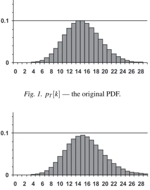
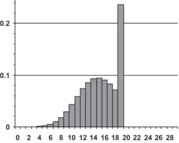
Fig. 1 and Fig. 2 show the original PDF and the result of the repeated convolutions, respectively. It can be observed that the expected value of the PDF was slightly moved to the right. Fig. 3 shows the result of the capacity thresholding.
Fig. 1. pTk]— the original PDF.
The distribution was limited to 20 cells num-bered from 0 to 19. In more than 23% of the cases the utilisation is 100%. The original value of cell 19 in Fig. 2 was 0:059, and 0:177 was
added to it due to the tail was cut off. Fig. 4 shows the PDF of the delay distrition. The probability of the 1 T delay is about 17:7%.
Fig. 3. PTk]— result of capacity thresholding.
Fig. 4. DTi]— delay distribution.
In the procedure above, we used histograms, with a cell size of 1. In the case of the bit-throughput histograms, and sometimes also in the case of the packet-throughput histograms, the size of the cells must be greater than one for efficiency. Then we need to consider the effect of the larger cell size and use the modified con-volution algorithm we will describe in the next chapter.
4. Discussion of Important Details
4.1. The Effect of the Finite Cell Size
If the size of the cells of the histogram is negligi-ble, the convolution is trivial(Fig. 5 and Fig. 6).
If the size of the cells of the histogram is not negligible, the convolution behaves like Fig. 7 and Fig. 8 show. The explanation is the fol-lowing: Letw denote the size of the cells. We number the cells from 0. The position of the
i-th cell is: iw(i+1)w], the position of the
j-th one is: jw(j+1)w], the position of the
Fig. 5.Density functions to add — ideal case.
Fig. 6.The result of the convolution — ideal case.
Fig. 7.Density functions to add — the cell size is not negligible.
middle points of the cells are: (i+0:5)w and
(j+0:5)w. The position of the resulting cell
is then: (i+j)w(i+j+2)w], that is exactly
the place of the(i+j)-th plus the(i+j+1)-th
cells. As the width of the resulting cell is 2wthe height of the cell must be divided by 2, so the result of the convolution remains a normalised probability density function.
4.2. Routing Units
When determining thesize of the routing unit
(SRU)we must consider the following issues:
The largerSRU we choose, the fewer messages are to be routed in the first phase and the less traffic model addition is to be performed in the second phase of TFA. However, if SRU is too large, the spatial distribution of the traffic may considerably differ from the one that is formed in the detailed simulation(and in the real
sys-tem). IfSRU is small, the spatial distribution of
the traffic may be quite precise, but the larger amount of messages to be routed and traffic models to be added slow down analysis. The
choice of SRU must be a reasonable
compro-mise that is made in the knowledge of the whole
system modelled.
The author would like to highlight another im-portant feature of TFA now. The facts thatSRU can be chosen for the applications of different types independently, and SRU < 1 is possible
assure the following advantage: if there is an application A whose traffic is just a small por-tion of the traffic of another applicapor-tion B, but for some reason it is very important for us to know its spatial distribution, TFA has an addi-tional comparative advantage over the detailed simulation. In this case, one has to continue the detailed simulation until he can collect enough samples from the traffic of application A. Mean-while the detailed simulation transfers much more from the traffic of the application B than it would be necessary for the statistics collection. If we use TFA and choose the value ofSRU for all the application types well, not much more has to be transferred from the traffic of any type of applications than it is necessary. This way TFA may serve theimportance sampling.
5. Application of TFA - an Example
Let us use a commercial network as an illustra-tion of the applicaillustra-tion of the method. A num-ber of different types of applications may use the network such as POS(Point Of Sale), ATM
(Automatic Teller Machine), file transfer, alarm
systems, etc. For TFA, all these applications will be modelled by the General Application Model(GAM). The most important parameter
of the GAM is the type of the applications it represents. The traffic generated by the GAM is determined by a number of parameters that are defined for all the different types of appli-cations.
As it was mentioned before, we use aggregated traffic model, so the GAM is able to represent the traffic of all the applications of its type(that
are connected to the given node). If the
rout-ing algorithm for the propagation of packets is symmetrical i.e. the same from A to B as from B to A, then the traffic between A and B can be handled together and the combined traffic is propagated from A to B. For example: a “client” generates the traffic model that describes its traf-fic towards one or more “servers” that receive the traffic model but generate no reply because the traffic model sent by the client represents the traffic of both directions(sent and received
by the client).
5.1. The Parameters of the GAM
We estimate the number of the different types of applications in the network, as well as their spatial distribution, and the time distribution of their activity during the day. In addition to that, for TFA, we have to determine what size of traffic can be handled together. Hence, the pa-rameters of the GAM are:
NApp(type) Number of Applications — the
number of all the applications of the given type
NAppPN(type, node)Number of Applications
Per Node — the number of all the applica-tions of the given type connected to the given node
PAc(type, day, time)Probability of Activity
SRU(type)Size of Routing Unit — the
max-imum size of the unit of the traffic(that can
be handled together) for the given type of
application
The reader may have noticed that for the de-scription of the users’ behaviour we consider the time of day and distinguish the days of the week too. The latter is justified, for example, by the different behaviour of the users on working days and on holidays. Of course, it is possible that for some applications the users’ behaviour depends on the position of the day within the month or in the season, but because this would give no theoretical novelty, we avoid the usage of unnecessarily many parameters.
The GAM generates traffic according to the number of the active applications:
NApp(typenodedaytime)
=
NApp(typenode)PActypedaytime)
NApp(type)
and issues the traffic(model)in at mostSRU(ty;
pe)size of units, where NApp and SRU are not
necessarily integers.
The traffic of the GAM can be categorized into a given number oftransaction types(
abbrevi-ated astt). The transactions are the basic units
of the traffic in our model of the considered commercial network.
5.2. Elimination of the Time Change within The Transactions
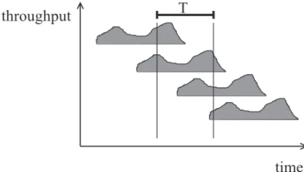
In our model, we suppose that the time change of the intensity of the transaction generation is relatively slow compared to both the T size of the throughput collection interval and the dura-tion of the transacdura-tions. So we consider that the starting time of the transactions in aT interval has a uniform distribution. Moreover, distribu-tion of the starting time of the transacdistribu-tions was very similar just before the beginning of thatT
interval. In this way, we may say that in a well chosenTinterval we take into consideration the whole traffic of the transactions beginning in thatT time interval.
Fig. 9.The elimination of the time change within the transactions — illustration.
5.3. Parameters of the GAM
Transactions of the GAM are also described by parameters. The parameters express what load the transactions of a given type cause for the lines and nodes, how many of them occur a day, and what their time distribution within the day is. The parameters of the transactions are:
Nfsjrg
b (tt)Number of Bits Sent | Received —
the number of bits sent or received by the application during a transaction of the given type
Nfsjrg
p (tt)Number of Packets Sent | Received
— the number of packets sent or received by the application during a transaction of the given type
Nc(tt)Number of Connection Set-ups — the
number of connections set-ups performed by the application during a transaction of the given type, typically 0 or 1, if this is possi-ble at all(for connection oriented protocols
only)
NTrPD(tt, day)Number of Transactions Per
Day — the number of transactions performed by an application of the given transaction type on a given day of the week
ITr(tt, day, time) Intensity of Transaction
generation — the value of the PDF at the given time that PDF describes the time dis-tribution of the transactions of the given type on the given day of week.
Remarks:
cause significant load for the nodes(
switch-es). E.g. the load caused by a connection
set-up may equal the load of the switching of 10 packets. This is the reason for intro-ducing the parameterNc.
2. ITr is defined for all the days of the week when there are transactions of the given type. Being a probability density function:
243600 Z
time=0
ITr(ttdaytime)=1
(the time is measured in seconds).
5.4. Transaction Generation with Poisso-nian Distribution
In our model, the active applications generate transactions according to a Poissonian process with parameter λ, that means the inter-arrival time has an exponential distribution with param-eterλ. Thus, the probability that k transactions are generated inT time is:
pTk]= (λT)
k
k! e
;λT :
The intensity of the transaction generation is:
λ(ttnodedayt)
=
NAppPN(typenode)NTrPD(ttday)
NApp(type)
ITr(ttdaytime)
Remark: as the transaction type(tt)determines
the application type(type),typecan be omitted
iftt is included.
Therefore the traffic model is built up by the transaction type-wiseλ,Ns
b,Nbr,Nps,Nrp,Nc pa-rameters.
5.5. Addition
Let us exploit the possibilities for simplifica-tion. Considering that the sum of two Poisso-nian distribution variables has also PoissoPoisso-nian distribution we can numerically add the λ val-ues of the same transaction type. (Either they
came from different sources or from the same
one, but were carried by a separate routing unit.)
Consequently, the network elements may col-lect the statistics of the transmitted traffic into a single scalar intensity variable for each transac-tion type. This is an important result, because thus we use scalar addition operations only(and
not convolutions)during the spatial distribution
phase.
While intensity values can be simply added up in the case of transactions of the same type, this cannot be done with transactions of different types as theirNs
b,Nbr,Nps,Nrp,Ncparameters may differ. Let us consider the sent bit-throughput as an example. We get the sent bit-throughput histogram from the histogram of the Poissonian distribution with parameter λ(tt) by
multiply-ing the cell width and dividmultiply-ing the cell height by
Ns
b(tt). These sent bit-throughput histograms
are then added up by convolution for all the transaction types.
The calculation is still not finished. To get the traffic of a line in one direction, we must add up the cumulated sent bit-throughput histogram of the given direction and the cumulated received bit-throughput histogram of the other direction. The capacity thresholding should be done the same way as described in 3.3.
5.6. Questions of the Efficient Implementation
To speed up the execution of TFA, we applied sometimesεvalues(given as parameters)to
ex-press the accuracy expected by the user. These are as follows:
εP Epsilon of Poissonian Tail— It is used when calculating the histogram of the Pois-sonian distribution from the transaction type-wise cumulatedλ value. If pTk] < εP for
a givenk, then the tail of the distribution is omitted fromk.
εA Epsilon of Addition — It is used to bound the result of the convolution in the above-mentioned manner. Without this, the number of the small probability cells could grow beyond measure so as the computation requirement of the further convolutions.
difference of pTk]
2 and the original p
Tk]:
firstChange. After each step we calculate the difference of pTk]
iandp Tk]
(i;1)
: actu-alChange. We may stop when:
actualChange<εCf irstChange:
As for efficiency, another important issue is the quantity of the human work used for the anal-ysis. To be economical with this, we have pre-pared an object-oriented library. Various ob-jects e.g. traffic generator, line, node, traffic sink, etc. are C++ classes with pure virtual
functions that are defined when implementing the layer 3 protocol of the analysed network. This solution requires less amount of work from the person who implements the model than us-ing only a predefined library of functions.
At present we do not apply it, but in the future the convolutions may be eliminated by using FFT and FFT;1transformations. It returns
es-pecially when the resolution of the histograms and/or the number of convolutions are high.
As a module of the Iminet network expert sys-tem, a TFA implementation applicable for the fast analysis of commercial networks was pre-pared for the Elassys Consulting Ltd.
6. Comparison of TFA and the Pure Analytical Method
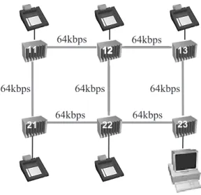
We use a simple network with 6 nodes for the comparison of the two methods. The nodes are connected by 64kbps lines according to the topology shown in Fig. 10. A server is con-nected to one of the nodes and is used by the terminals connected to the 5 other nodes. There are 150 terminals per node, and they are active with the probability of 60%. When they are active, they perform about 2 transactions per minute. One transaction of the terminals con-tains 5 sent and 4 received packets. The length distribution of the packets is uniform in the140
byte, 180 byte]interval.
Fig. 10.Topology of the network(Iminet graphics).
The nodes of the network are X.25 switches that use no fixed routing table rather adaptive algorithm. They find the minimal cost route for every new connection according to the fol-lowing conditions: there is a fixed switching cost (CSw) for every switch the path contains,
and the cost for the contained lines is in direct proportion to the number of already existing connections on the line. The factor isCpC(cost
per connection).
Let us determine the parameters of the TFA model. There is a single application type with one transaction type only, thus thetypeandtt pa-rameters will be omitted. The number of appli-cations in the system is: NApp=5150=750.
The 5 nodes each haveNAppPN = 150 number
of terminals that are active with the probabil-ity of PAc = 0:6. During a single transaction
the application sendsNbs = 6400 and receives
Nr
b = 5120 bits. The number of packets sent
is: Ns
p = 5, the number of packets received is:
Npr = 4, the number of connection set-ups is:
Nc = 1, and the number of all the transactions
per day is:
NTrPD =NAppPAc(2=60)243600
that is
NTrPD =1586400
value of the density function is constant all over the day:
ITr 1=86400
The size of the routing unit(SRU)is an
impor-tant parameter of the analysis, we executed TFA using different values for it.
Table 1, Table 2, and Table 3 show the results for the utilisation of the lines. We calculated the analytical values of the average utilisation of the lines and we give them in the first column for comparison. (Naturally, they are identical
in all the 3 tables.) To save space, only the
line anal. average s. dev. min. max. 11!12 15360 15337 66.5 15104 15488
12!13 23040 23009 108.8 22699 23232
21!22 23040 23063 127.5 22912 23296
22!23 53760 53792 153.9 53568 54101
11!21 3840 3863 167.6 3712 4096
12!22 11520 11528 178.3 11328 11626
13!23 42240 42209 198.0 41899 42432
Table 1.Line utilisation values —SRU=0:1.
line anal. average s. dev. min. max. 11!12 15360 15181 378.4 14080 15787
12!13 23040 22859 533.1 21333 23680
21!22 23040 23219 653.7 22613 24320
22!23 53760 53941 753.9 53120 55467
11!21 3840 4019 843.5 3413 5120
12!22 11520 11522 881.1 10453 12160
13!23 42240 42059 957.8 40533 42880
Table 2.Line utilisation values —SRU=1.
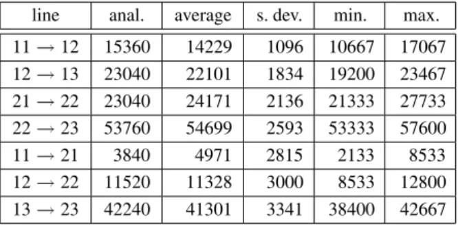
line anal. average s. dev. min. max. 11!12 15360 14229 1096 10667 17067
12!13 23040 22101 1834 19200 23467
21!22 23040 24171 2136 21333 27733
22!23 53760 54699 2593 53333 57600
11!21 3840 4971 2815 2133 8533
12!22 11520 11328 3000 8533 12800
13!23 42240 41301 3341 38400 42667
Table 3.Line utilisation values —SRU=10.
sent bit-throughput is presented, the received bit-throughput carries no further information concerning the spatial distribution of the traf-fic. As the application models wait for a ran-dom delay between the sending of the constive routing units, the result of TFA depends on the actual representation of these random numbers. We performed TFA a great number of times, averaged the results, computed the standard de-viation, determined the minimum and the max-imum values. As we will not have “analyti-cal values” when applying TFA for a real life problem, we used the formula of the empirical deviation:
σ = v u u u t
N P i=1
(xi; x)
2
N;1
Examining the results, we can point out that in the case ofSRU = 0:1, the deviation is always
less than 5with higher load it is less than 1%, or even 0:5%. The difference between the
mini-mal and maximini-mal values is little, thus in this case a single experiment gives good approximation with high probability.
In the case of SRU = 10 the average values
are still good approximations of the analytical values (except for the 11 ! 21 line) but the
minimal and maximal values differ much, thus in this case really a great number of experiments are needed. Let us examine what causes the sig-nificant difference from the analytical value for the 11 ! 21 line. The analytical method has
shown that this line carries only 18 transactions
(in expected value). Naturally, this value
can-not be approximated well in the caseU = 10.
The problem can be handled by decreasingSRU and/or increasing the number of experiments,
but it is not always necessary. In this partic-ular case if we do not intend to decrease the line capacity below 64kbps just wish to decide whether 64kbps is enough for all the lines, the exact bit rate values of a lines are not important for us if we know they are much less than the line capacity.
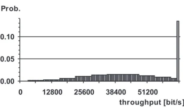
Besides the average, let us examine the bit-throughput distributions and delay distributions of the lines. Let us select two interesting lines. The first one is line 22 ! 23. The analytical
is higher than the 80% of the 64kbps that is con-sidered to be safe according to the well-known rule of thumb.
Fig. 11.The bit-throughput distribution of line 22!23.
Fig. 12.The delay distribution of line 22!23.
Fig. 13.The bit-throughput distribution of line 13!23.
Fig. 14.The delay distribution of line 13!23.
A Fig. 11 shows the bit-throughput distribution of line 22!23. It is conspicuous, that the line
is fully utilised with nearly 50% probability. It results in the delay distribution is displayed in Fig. 12. The application of a 128k line is worth considering here.
Fig. 13 shows the bit-throughput distribution of line 13 ! 23. Here, the probability of 100%
utilisation is less than 14%. The delay distribu-tion(Fig. 14)can be considered as acceptable.
In the case of the other lines, full utilisation has no significant probability thus the analysis of their traffic is of no interest for us.
This example demonstrated how TFA could be used for revealing bottlenecks in a network.
7. Conclusions
The reader was introduced to the traffic-flow analysis describing its networking model, gen-eral operation and capabilities enlarging upon the selected traffic model and its operations. After the discussion of some critical details an actual implementation of TFA was presented. Finally, a case study was given comparing the results of TFA to those of the pure analytical method. We have found that the results of TFA approximate well the results of the pure analyt-ical method.
We conclude that TFA can be an efficient method for the fast approximate performance analysis of large communication systems.
The direction of the future research may be the comparison of TFA and the detailed simulation applying them for the analysis of more complex networks (that cannot easily be studied in the
analytical way) concerning both the accuracy
of the results and the execution time.
8. Acknowledgements
The results recited in this paper arose from the R&D project of Elassys Consulting Ltd that deals with information technology and simu-lation of communication systems.
References
1] BANKS, J.; J. S. CARSON; B. L. NELSON
Discrete-Event System Simulation. Prentice Hall, Upper Sad-dle River, New Jersey, 1996.
2] BRATLEY, P.; B. L. FOX; AND L. E. SCHRAGE A
Guide to Simulation. Springer-Verlag, New York, 1986.
3] FUJIMOTO, R. M. Parallel Discrete Event
Simula-tion.Communications of the ACM 33(1990), no.
10, pp. 31-53
4] JAIN, R.; ANDI. CHLAMTACThe P
2 Algorithm for Dynamic Calculation of Quantiles and Histograms Without Storing Observations.Communications of the ACM28(1985), no. 10, pp. 1076-1085.
5] JAIN, R.The Art of Computer Systems Performance
Analysis. John Wiley & Sons, New York, 1991.
6] J ´AVOR, A. (editor) Simulation in Research and
Development. North-Holland, Amsterdam, 1985.
7] J ´AVOR, A. Petri Nets in SimulationEUROSIM
Sim-ulation News Europe, 1993, no. 9, pp. 6-7.
8] JEFFERSON, D; B. BECKMAN; F. WIELAND; L.
BLUME; M. DILORETO; P. HONTALAS; P. LAROCHE;
K. STURDEVANT; J. TUPMAN; V. WARREN; J. VEDEL;
H. YOUNGER ANDS. BELLENOT. Distributed
Simu-lation and the Time Warp Operating System. Pro-ceedings of the 12th SIGOPS — Symposium on Operating System Principles,(1987), pp. 73-93.
9] LENCSE, G. Efficient Parallel Simulation with the
Statistical Synchronization Method.Proceedings of the Communication Networks and Distributed Sys-tems Modeling and Simulation (CNDS’98), San Diego, CA.(1998. Jan. 11-14)SCS International,
pp. 3-8.
10] LENCSE, G. Statistics Collection for the Statistical
Synchronisation Method.Proceedings of the 10th European Simulation Symposium (ESS’98), Not-tingham, UK.(1998. Oct. 26-28)SCS Europe, pp.
46-51.
11] LENCSE, G. Applicability Criteria of the
Statisti-cal Synchronization Method. Proceedings of the Communication Networks and Distributed Systems Modeling and Simulation (CNDS’99), San Fran-cisco, CA. (1999. Jan. 17-20) SCS International,
pp. 159-164.
12] PONGOR, GY. Statistical Synchronisation: a
Differ-ent Approach of Parallel Discrete EvDiffer-ent Simulation.
Proceedings of the 1992 European Simulation Sym-posium (ESS’92), Dresden, Germany.(1992. Nov.
5-8)SCS Europe, pp. 125-129.
13] VARGA, A; AND BABAK FAKHAMZADEH The
K-Split Algorithm for the PDF Approximation of Multi-Dimensional Empirical Distributions without Storing Observations. Proceedings of the 9th Eu-ropean Simulation Symposium(ESS’97), Passau,
Germany. (1997. Oct. 19-22) SCS Europe, pp.
94-98.
14] VARGA, A. K-split — On-Line Density Estimation
for Simulation Result Collection. Proceedings of the 10th European Simulation Symposium (ESS’98),
Nottingham, UK.(1998. Oct. 26-28). SCS Europe,
pp. 41-45.
Received:May, 2000
Accepted:September, 2000
Contact address:
G´abor Lencse Department of Telecommunications Sz´echenyi Istv´an University of Applied Sciences H´ederv´ari u. 3. H-9026 Gy¨or Hungary e-mail:[email protected] http://www.hit.bme.hu/phd/lencse