UNDERSTANDING SPECIES DISTRIBUTION AND DIVERSITY: INSIGHTS FROM TEMPORAL OCCUPANCY
Sara Jeanne Snell Taylor
A dissertation submitted to the faculty at the University of North Carolina at Chapel Hill in partial fulfillment of the requirements for the degree of Doctor of Philosophy in the Department
of Biology.
Chapel Hill 2020
ii © 2020
Sara Jeanne Snell Taylor ALL RIGHTS RESERVED
iii ABSTRACT
Sara Jeanne Snell Taylor: Understanding species distribution and diversity: insights from temporal occupancy
(Under the direction of Allen H. Hurlbert)
Understanding the processes underlying community assembly is one of the primary
goals of ecology. Studying communities can be complex because they often encompass a diverse
array of interacting taxonomic groups and trophic levels. Additionally, community makeup
changes in response to disturbances, environmental factors, interspecies interactions, and
anthropogenic alterations to habitat. Despite these challenges, discovering the drivers of
community assembly and dynamics will improve our ability to understand how ecosystems
function and conserve biodiversity effectively.
Typically, characterizing community assembly uses species abundance, which
provides information about which species are currently present in the community, but does not
address which species are consistent members of a community versus species poorly suited to the
habitat they are observed in. This distinction is critical when considering questions such as
estimating community biodiversity, community composition, and temporal turnover. One way to
address this issue is by using the metric of temporal occupancy, or how frequently a species is
observed at a given site within its community.
To understand how temporal occupancy affects our understanding of ecological
systems, I tested the prevalence and impact of species who appear infrequently in their
iv
distributions, species richness correlation with environmental heterogeneity, temporal turnover,
and species-area relationships using 7 taxonomic groups.
Once these patterns have been examined from the perspectives of transient and
non-transient species from a diversity of communities, I investigated the abiotic and biotic
determinants of avian temporal occupancy in North America. Then, I applied the metric of
temporal occupancy to commonly used species distribution models (SDMs) to determine
whether avian species distributions are better predicted using temporal occupancy as opposed to
presence and absence.
Finally, I tested whether temporal occupancy provides robust inferences for
identifying core and transient species using simulations. I simulated species dynamics over time
with varying habitat heterogeneity and detection to understand core and transient structure within
a community without the added noise of a biological system. Together, these studies improve
scientific insight into community ecology and allow us to predict how communities will respond
v
vi
ACKNOWLEDGEMENTS
First, I would like to thank my advisor, Allen Hurlbert, for his dedicated mentorship over the course of my graduate career. He encouraged me to become a thoughtful and
independent scientist by providing insightful feedback on thoughts and ideas and imparting a strong foundation for coding, which has become my passion in graduate school. His feedback also helped me become a stronger writer and presenter. Additionally, I am deeply grateful to my committee; John Bruno, Charles Mitchell, James Umbanhowar, and Ethan White, for their feedback and support throughout graduate school. John Bruno enthusiastically supported my research and provided valuable feedback on my ideas and visualizations. Charles Mitchell provided thoughtful comments for all of my chapters and was eager to discuss ideas with me throughout my graduate career. James Umbanhowar provided statistical support for each of my chapters and was always available to discuss statistical issues or coding problems. Ethan White provided macroecological and avian expertise for each of my projects, helping shape the primary questions of several of my chapters.
vii
I am grateful to my lab mates, Robbie Burger, Molly Jenkins, and Grace Di Cecco, who have enriched my professional and personal experience in graduate school. Robbie Burger was instrumental in helping me develop ideas in my first years of graduate school, and helped me navigate through each graduate school milestone, even when he had moved on to new positions. Molly Jenkins provided helpful feedback on manuscripts and presentations in my first years of graduate school, as well as maintained an infectiously positive presence in the lab. Finally, Grace Di Cecco has been a strong collaborator and great friend. We have collaborated on multiple projects, including a chapter of my dissertation, and I am excited to continue working with her on future projects.
I am incredibly grateful to my family and friends, whose support was instrumental throughout graduate school. My parents, Terry and Sandra Snell, instilled an early love of
biology in me and have supported me in every personal and professional endeavor. Thank you so much for always being available to talk, sending care packages and cards, and always keeping a positive perspective. I am also incredibly grateful to my in-laws, Sheldon and Ann Taylor, who have enthusiastically supported me throughout college and graduate school and warmly
viii
ix
TABLE OF CONTENTS
LIST OF TABLES ... xii
LIST OF FIGURES ... xiii
CHAPTER 1: INTRODUCTION ... 1
REFERENCES ... 4
CHAPTER 2: THE PREVALENCE AND IMPACT OF TRANSIENT SPECIES IN ECOLOGICAL COMMUNITIES ... 6
INTRODUCTION ... 6
METHODS ... 9
Data ... 9
Analysis ...11
RESULTS ...15
DISCUSSION ...17
Impacts of Transient Species on Ecological Inference ...20
Considerations ...23
Conclusions ...25
x
CHAPTER 3: THE RELATIVE IMPORTANCE OF BIOTIC AND ABIOTIC DETERMINANTS OF TEMPORAL OCCUPANCY FOR AVIAN SPECIES IN
NORTH AMERICA ...37
INTRODUCTION ...37
METHODS ...39
Bird data ...39
Biotic drivers ...40
Abiotic drivers ...41
Temporal occupancy and detectability...42
Analysis ...44
Competitor null model ...46
RESULTS ...47
DISCUSSION ...51
REFERENCES ...57
CHAPTER 4: DOES TEMPORAL OCCUPANCY PREDICT AVIAN SPECIES DISTRIBUTIONS BETTER THAN PRESENCE-ABSENCE? ...67
INTRODUCTION ...67
METHODS ...69
RESULTS ...72
DISCUSSION ...74
xi
CHAPTER 5: DOES TEMPORAL OCCUPANCY PROVIE ROBUST INFERENCES FOR IDENTIFYING CORE AND TRANSIENT SPECIES? AN INFERENCE
CHECK FOR TEMPORAL OCCUPANCY SIMULATIONS ...87
INTRODUCTION ...87
METHODS ...89
Simulation model ...89
Simulation analysis ...91
RESULTS ...92
DISCUSSION ...93
REFERENCES ...98
CHAPTER 6: CONCLUSION... 107
REFERENCES ... 111
APPENDIX A: SUPPLEMENTARY MATERIAL FOR CHAPTER 2 ... 112
Sampling standardization of community time series datasets ... 112
Null model analysis of species abundance distributions and temporal turnover ... 113
Supplemental tables and figures ... 117
APPENDIX B: SUPPLEMENTARY MATERIAL FOR CHAPTER 3... 125
xii
LIST OF TABLES
Table 3.1: Bayesian hierarchical model results for the fixed effects of environmental z-score and competitor abundance on focal species temporal occupancy. ...61 Table 3.2: Regression model of the effect of continuous traits
and categorical traits on logit-transformed RC. ...61
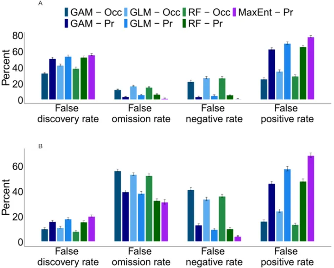
Table 4.1: Definitions of error rates and the best performing input variable for each
cross-validation metric. ...81
Table 5.1: Table of terminology for each classification of temporal occupancy and
population viability discussed in the simulation output. ... 100
Table A2.1: Linear mixed model results for the effect of elevational heterogeneity, taxa, and community size on the proportion of transient species. ... 117
Table C4.1: Paired t-tests for each temporal validation error rate using all three model types (GLM/GAM/RF), comparing temporal occupancy and presence SDMs. ... 132 Table C4.2: Paired t-tests for each spatial validation error rate using all three model types
xiii
LIST OF FIGURES
Figure 2.1: Schematic of properties of transient species. ... 32 Figure 2.2: Description of the compiled time-series datasets. ...33 Figure 2.3: The mean proportion of species in an assemblage that are transient, core, or
intermediate. ...34 Figure 2.4: Linear models of the proportion of transient species as a function of sample area and sample community size for hierarchically scaled datasets and rescaled proportion of
transients using median community size. ...35 Figure 2.5: Comparison of common ecological patterns between full communities and
communities excluding transient species. ...36 Figure 3.1: Violin plots demonstrating the distribution of unique variance in focal temporal occupancy explained by environmental variables, summed abundance of all competitors, and Rc for all and main competitor abundance. ...62
Figure 3.2: The top 15 focal species ranked by variance explained by scaled competitor
abundance. ...63 Figure 3.3: The top 15 focal species ranked by variance explained by deviation from optimal environmental conditions. ...64 Figure 3.4: The ability of environmental variables, competitor abundance, or both combined to predict spatial variation in temporal occupancy compared to spatial variation in abundance based on linear regression R2s. ...65
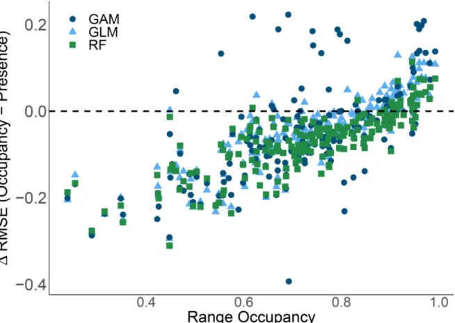
Figure 3.5: Competitor null model analysis for one and all focal species. ...66 Figure 4.1 Map depicting 11 SDMs of the Yellow-throated Vireo. ...82 Figure 4.2 Comparisons of root mean square error (RMSE) for species distribution models using temporal occupancy based on 15-years of data versus presence. ...83 Figure 4.3: Comparisons of root mean square error (RMSE) for species distribution models using temporal occupancy based on 5-years of data versus presence. ...84 Figure 4.4: Plot of the difference of each species’ RMSE for temporal occupancy – presence SDM output versus range occupancy. ...85 Figure 4.5: Average error rates (+/- standard error) across all species for temporal
xiv
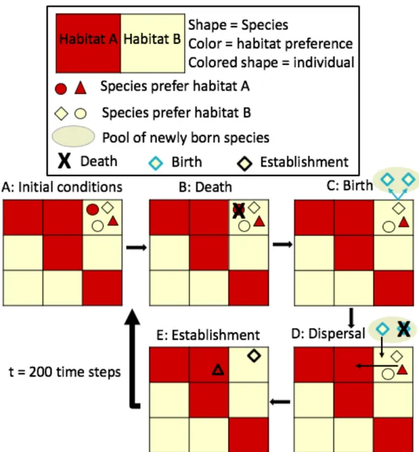
Figure 5.2 Schematic demonstrating how error rates are calculated on the simulation results. . 102
Figure 5.3: Sample landscape of one simulation run using two sets of parameters. ... 103
Figure 5.4: Mean number of biologically core and biologically transient species richness for each combination of detection probability and landscape similarity... 104
Figure 5.5: Percent of biologically core species that were incorrectly inferred to be transient and biologically transient species that were incorrectly inferred to be core. ... 105
Figure 5.6: Distribution of abundance of biologically core species correctly (black) and incorrectly (grey) classified using temporal occupancy. ... 106
Figure A2.1: A hypothetical dataset with 3 sites that have been sampled with variable intensity over time and the subsampling threshold is the smallest value for which the % of available site-years exceeds 50%. . ... 113
Figure A2.2. Null model analyses of Figue 2.5A. ... 115
Figure A2.3. Null model analyses of Figure 2.5C. ... 116
Figure A2.4. Visualization of each data subsets used for analyses in the manuscript. ... 118
Figure A2.5. The impact of different thresholds on the proportion of transient species in assemblages from different taxonomic groups. ... 119
Figure A2.6. The impact of scale on the proportion of transient species as in Figure 2.4 , where transient species are defined as those with temporal occupancy ≤ 10%. ... 120
Figure A2.7. The impact of scale on the proportion of transient species as in Figure 2.4 , where transient species are defined as those with temporal occupancy ≤ 25%. ... 121
Figure A2.8. Impact of excluding transient species on four ecological patterns as in Figure 2.5, where transient species are defined as those with temporal occupancy ≤ 10%... 122
Figure A2.9. Impact of excluding transient species on four ecological patterns as in Figure 2.5, where transient species are defined as those with temporal occupancy ≤ 25%... 123
Figure A2.10. Turnover calculation using Bray-Curtis index rather than the Jaccard index used in Figure 2.5C.. ... 124
Figure B3.1.Relationships between temporal occupancy and NDVI. ... 125
Figure B3.2. Comparison of estimates below and above the Centroid NDVI. ... 126
xv
Figure B3.4. The ability of environmental variables, most widespread competitor abundance, or both combined to predict spatial variation in temporal occupancy
compared to spatial variation in abundance based on linear regression R2s. ... 128
Figure B3.5. The ability of environmental variables, most predictive competitor abundance, or both combined to predict spatial variation in temporal occupancy
compared to spatial variation in abundancebased on linear regression R2s. ... 129
1
CHAPTER 1: INTRODUCTION
Characterizing how species assemble is critical for determining why species persist at
sites within in their range (Cody & Diamond, 1975; Connor & Simberloff, 1983). Generally,
species require specific environmental conditions to succeed in a particular habitat, but often
they do not occur everywhere the environment is suitable (Hutchinson 1957, Chesson 2000,
Gaston 2003). This discrepancy could be due a number of factors other than the environment,
ranging from biotic interactions to dispersal ability. Determining how species are affected by
environmental and biotic conditions can allow us to understand how species assemble within
their communities as well as how they persist throughout their range.
Traditional terrestrial species distribution analyses have used environmental factors such
as temperature, precipitation, elevation, and tree cover as the primary determinants of whether a
species would be able to survive in a habitat and what combination of factors would form its
optimal climate (Guisan & Thuiller, 2005; Johnson, 1924). More recently, studies have
demonstrated that including interspecific interactions can create a more complete and accurate
species distribution models (Belmaker et al., 2015; Bruno et al., 2003; Guisan & Thuiller, 2005)
and that biotic factors such as interspecific interactions can strongly determine species ranges,
even at large scales (Belmaker et al., 2015; Mönkkönen et al., 2017; Ricklefs, 2012). Therefore,
considering both environmental limitations as well as biotic factors is necessary to fully describe
2
Traditionally, species distributions were modeled in terms of presence/absence (Diamond
& Hamilton, 1980; McCoy & Heck, 1987) or as a snapshot in time of spatial abundance patterns
(Mönkkönen et al., 2017), providing limited information about the temporal structure of the
community. More recently, several studies have considered the temporal structure of
communities by using temporal occupancy, the frequency with which a species occurs at a given
site, and demonstrate unique information about species distribution and community assembly
(Magurran and Henderson 2003, Ulrich and Ollik 2004, Coyle et al. 2013, Supp et al. 2015,
Umaña et al. 2017, Snell Taylor et al. 2018). Considering both temporal and spatial aspects is
critical when considering ecological community patterns and I seek to determine when to use
temporal occupancy in ecological analyses, how temporal occupancy performs relative to other
occurrence metrics, and how often the differences in temporal occurrence within communities
affects ecological patterns.
One question well suited for temporal occupancy data is how to characterize diversity
and composition of ecological communities. The traditional method for studying community
composition is through taxonomic surveys monitored over time. We typically assume that
species observed in taxonomic surveys are regular inhabitants of a local population, yet new
evidence shows that some species may be irregular visitors that are poorly suited to the local
conditions, have negative local population growth rates, and rarely interact with other members
of the community (Taylor et al., 2018). Grinnell (1922) first coined the term "accidental" to refer
to this kind of species, which is observed inconsistently at a site over time in contrast to the more
regular and predictable members of an assemblage. Subsequent authors have referred to them as
"occasional", "vagrant", "transient", "tourist", or "sink" species, and they have been observed in
3
Magurran & Henderson, 2003; Novotný & Basset, 2000; Petersen et al., 2015; Pulliam, 1988;
Southwood et al., 1982; Supp et al., 2015; Ulrich & Ollik, 2004). These species are unique from
resident, or core, community members and the only method to detect them is surveying sites over
multiple time points.
In this dissertation, I used temporal occupancy to gain a comprehensive view of the
drivers of community assembly and determinants of species range. First, I analyzed how
transient species affect community assembly across multiple taxa and ecosystems to gain a sense
of how prevalent these species are in their communities. Second, I considered how abiotic and
biotic factors determine avian temporal occupancy across North America. Third, I quantified
how using temporal occupancy or presence and absence affected avian species distribution
4
REFERENCES
Belmaker, J., Zarnetske, P., Tuanmu, M.-N., Zonneveld, S., Record, S., Strecker, A., &
Beaudrot, L. (2015). Empirical evidence for the scale dependence of biotic interactions.
Global Ecology and Biogeography, 24(7), 750–761.
Bruno, J. F., Stachowicz, J. J., & Bertness, M. D. (2003). Inclusion of facilitation into ecological theory. Trends in Ecology & Evolution, 18(3), 119–125.
Chesson, P. (2000). General Theory of Competitive Coexistence in Spatially-Varying Environments. Theoretical Population Biology, 58(3), 211–237.
Cody, M. L., & Diamond, J. M. (1975). Ecology and Evolution of Communities. Harvard University Press.
Connor, E. F., & Simberloff, D. (1983). Interspecific Competition and Species Co-Occurrence Patterns on Islands: Null Models and the Evaluation of Evidence. Oikos, 41(3), 455–465.
Costello, M. J., & Myers, A. A. (1996). Marine Biodiversity Turnover of transient species as a contributor to the richness of a stable amphipod (Crustacea) fauna in a sea inlet. Journal of Experimental Marine Biology and Ecology, 202(1), 49–62.
Coyle, J. R., Hurlbert, Allen H., & White, E. P. (2013). Opposing Mechanisms Drive Richness Patterns of Core and Transient Bird Species. The American Naturalist, 181(4), E83–E90.
Diamond, A. W., & Hamilton, A. C. (1980). The distribution of forest passerine birds and Quaternary climatic change in tropical Africa. Journal of Zoology, 191(3), 379–402.
Dolan, J. R., Ritchie, M. E., Tunin-Ley, A., & Pizay, M.-D. (2009). Dynamics of core and occasional species in the marine plankton: Tintinnid ciliates in the north-west Mediterranean Sea. Journal of Biogeography, 36(5), 887–895.
Gaston, K. J. (2003). The Structure and Dynamics of Geographic Ranges (1st ed.). Oxford University Press.
Grinnell, J. (1922). The Role of The “Accidental.” The Auk, 39(3), 373–380.
Guisan, A., & Thuiller, W. (2005). Predicting species distribution: Offering more than simple habitat models. Ecology Letters, 8(9), 993–1009.
Hutchinson, G. E. (1957). Concluding Remarks. Population Studies: Animal Ecology and Demography. Cold Harbor Symposia on Quantitative Biology, 22, 415–427.
5
Magurran, A. E., & Henderson, P. A. (2003). Explaining the excess of rare species in natural species abundance distributions. Nature, 422(6933), 714–716.
McCoy, E. D., & Heck, K. L. (1987). Some Observations on the Use of Taxonomic Similarity in Large-Scale Biogeography. Journal of Biogeography, 14(1), 79–87.
Mönkkönen, M., Devictor, V., Forsman, J. T., Lehikoinen, A., & Elo, M. (2017). Linking species interactions with phylogenetic and functional distance in European bird assemblages at broad spatial scales. Global Ecology and Biogeography, 26(8), 952–962.
Novotný, V., & Basset, Y. (2000). Rare species in communities of tropical insect herbivores: Pondering the mystery of singletons. Oikos, 89(3), 564–572.
Petersen, E. D. S., Rossi, L. C., & Petry, M. V. (2015). Records of vagrant bird species in Antarctica: New observations. Marine Biodiversity Records, 8, e61 (6 pages).
Pulliam, H. R. (1988). Sources, Sinks, and Population Regulation. The American Naturalist,
132(5), 652–661.
Ricklefs, R. E. (2012). Habitat-independent spatial structure in populations of some forest birds in eastern North America. The Journal of Animal Ecology, 82(1), 145–154.
Southwood, T. R. E., Moran, V. C., & Kennedy, C. E. J. (1982). The Richness, Abundance and Biomass of the Arthropod Communities on Trees. Journal of Animal Ecology, 51(2), 635–649.
Supp, S. R., Koons, D. N., & Ernest, S. K. M. (2015). Using life history trade-offs to understand core-transient structuring of a small mammal community. Ecosphere, 6(10), 1–15. Taylor, S. J. S., Evans, B. S., White, E. P., & Hurlbert, A. H. (2018). The prevalence and impact
of transient species in ecological communities. Ecology, 99(8), 1825–1835.
Ulrich, W., & Ollik, M. (2004). Frequent and occasional species and the shape of relative-abundance distributions. Diversity and Distributions, 10(4), 263–269.
Umaña, M. N., Zhang, C., Cao, M., Lin, L., & Swenson, N. G. (2017). A core-transient
6
CHAPTER 2: THE PREVALENCE AND IMPACT OF TRANSIENT SPECIES IN ECOLOGICAL COMMUNITIES
INTRODUCTION
Ecologists frequently conduct taxonomic surveys to characterize the diversity and composition of ecological assemblages. While many of the species observed in these surveys represent local populations, some may be irregular visitors that are poorly suited to the local conditions, have negative local population growth rates, and rarely interact with other members of the community. Grinnell (1922) first coined the term "accidental" to refer to this kind of species, which is observed inconsistently at a site over time in contrast to the more regular and predictable members of an assemblage. Subsequent authors have referred to them as
"occasional", "vagrant", "transient", "tourist", or "sink" species (Southwood et al. 1982, Pulliam 1988, Costello and Myers 1996, Novotný and Basset 2000, Magurran and Henderson 2003, Ulrich and Ollik 2004, Dolan et al. 2009, Coyle et al. 2013, Petersen et al. 2015, Supp et al. 2015). By definition, a species with a negative population growth rate in a particular area is not
7
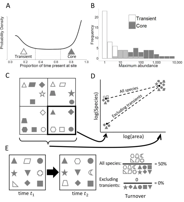
"core" species (Figure 2.1A; Costello and Myers 1996, Magurran and Henderson 2003, Coyle et al. 2013, Umaña et al. 2017). Unlike Hanksi’s core-satellite hypothesis that distinguishes species based on their spatial distribution, transient species are distinguished by their occurrence at a site over time, and species that are transient in one location may be core members of an assemblage elsewhere (Hanski and Gyllenberg 1993). The existence of a mode at low temporal occupancy indicates that transient species may make up a larger proportion of ecological assemblages than has typically been acknowledged.
Previous studiesfound that core species presence is more strongly tied to the
environment and other deterministic factors, while transient species presence is more strongly determined by stochastic factors (Magurran and Henderson 2003, Coyle et al. 2013, Umaña et al. 2017). Because much of the ecological theory related to species coexistence, niche partitioning, and biodiversity assumes that species directly interact and occur only in suitable environments, the presence of these transient species has the potential to skew our understanding of ecological systems. Indeed, transient species have been shown to differ from core species with respect to the shape of species abundance distributions (Figure 2.1B; Magurran and Henderson 2003), the relative importance of density-dependence versus environmental stochasticity (Magurran and Henderson 2003, Ulrich and Ollik 2004), the primary drivers of species richness (Coyle et al. 2013), and life history traits (Supp et al. 2015). We expect transient species may influence the slope of species-area relationships, since species that are transient may make up a
8
time (Figure 2.1E). Thus, a wide variety of classic ecological patterns may differ depending on whether transient species are considered, including biodiversity patterns that have the potential to influence conservation and management decisions.
Given the potential impact of transient species on understanding and managing ecological systems, it is important to understand more about how common transient species are and how their prevalence varies with taxonomic group, ecosystem types, environmental context, and scale. There are reasons to expect that several of these factors may influence the prevalence of transients. First, species from taxonomic groups with strong dispersal abilities like birds
commonly show up in habitats and regions in which they are not expected (Grinnell 1922, Coyle et al. 2013), whereas organisms with limited dispersal should do so much less frequently.
9
prevalence because the scale at which assemblages are sampled can vary by several orders of magnitude.
Here, we undertake the first systematic evaluation of the prevalence and predictors of transient species in ecological communities. We use data from over 19,000 community time series from terrestrial, aquatic, and marine ecosystems across seven major taxonomic groups to: 1) evaluate the prevalence of transient species and how it varies with taxonomic group,
ecosystem type, and habitat heterogeneity; 2) assess the scale-dependence of transient species prevalence and correct for scale to make consistent comparisons across groups; and 3) examine how the inclusion of transient species in community-level analyses impacts four commonly analyzed ecological patterns including the shape of species-abundance distributions, drivers of species richness, species-area relationships, and temporal turnover.
METHODS Data
10
11 Analysis
Following Coyle et al. (2013), we operationally defined a species as transient at a site if it was observed in 33% or fewer of the temporal sampling intervals, and assessed the
prevalence of transients as the proportion of species in the assemblage below this threshold (Figure 2.1A). We also evaluated more restrictive definitions using maximum temporal occupancy thresholds of 10% and 25% to evaluate the impact of this decision. Results were qualitatively similar for the three different thresholds (Figure A2.6-S6).
Although many authors have used the bimodality of temporal occupancy distributions (e.g., Figure 2.1A) to identify transient species in this way (Magurran and Henderson 2003, Dolan et al. 2009, Coyle et al. 2013), some species will be incorrectly classified due to imperfect detectability. Species with low detectability due to low density or traits or behaviors that make them difficult to detect may be persistent at a site but only detected in a small proportion of samples (MacKenzie et al. 2006, Henderson and Magurran 2014). As such, estimates of the proportion of transient species based on observed temporal occupancy are likely higher than the true numbers. A full exploration of the detailed influence of imperfect detection is beyond the scope of this paper, but we are developing simulation-based approaches to understand precisely how it influences estimates of the proportion of transients as well as the identification of
individual species (Hurlbert unpublished data).
12
regional habitat heterogeneity as would be expected of true transients while it was not positively correlated with vegetation which would be expected to impede species detections. In addition, similar studies using habitat preference-based transient designations (Belmaker 2009) have yielded similar conclusions to those using occupancy based approaches (Coyle et al. 2013). Finally, the results in this paper are similar for species that are comprehensively surveyed and those that are less thoroughly sampled (see Results and Considerations). So, while there is no doubt that misclassifications will occur, for large data compilations like this one that lack both detailed habitat preference data for species and the necessary sampling methods to estimate detection probabilities, occupancy based approaches appear to provide a reasonable approximate classification. We address these issues further in the Considerations section of the Discussion.
We evaluated the effect of spatial scale on the perceived prevalence of transient species using the subset of datasets that included sampling at hierarchically nested spatial scales (24 out of 88 datasets). We used a linear mixed model (lmer in the lme4 R package; Bates et al. 2015) to quantify how the proportion of transient species in an assemblage varied with the spatial scale (log-transformed sample area, a fixed effect) over which the assemblage was characterized, taxonomic group (a fixed effect), and the interaction between scale and taxonomic group,
allowing for random slopes and intercepts by dataset. For the three plankton datasets
13
that is more comparable than sampling area across groups. The lmer function output does not provide values due to uncertainties in the appropriate degrees of freedom. We calculated p-values by assuming that our sample sizes (in the thousands) were large enough such that the Wald’s t-values were effectively z-distributed (Luke 2017).
To assess how well our two measures of scale captured variation in the proportion of transient species, we calculated 1) the R2 for a simple linear model with scale as the sole
predictor, and 2) the marginal R2 (Nakagawa and Schielzeth 2013) for the mixed model
described above, which reflects the proportion of variance explained by only the fixed factors in the model. We focus primarily on comparing these values between our two scale measures rather than interpreting the absolute values themselves, which can be challenging for mixed effects models (LaHuis et al. 2014). Finally, we used our mixed model to generate predictions for how the proportion of transient species varies between taxonomic groups controlling for community size. We used a fixed community size of 102 individuals, the median community size for all assemblages.
To explore the influence of habitat heterogeneity on the prevalence of transient species in terrestrial assemblages we calculated the variance in elevation within a 5 km radius of each terrestrial assemblage using a 30 arc-second digital elevation model DEM of North America (GTOPO30), acquired from the USGS Earth Resources Observation and Science Center (EROS). We then fit a linear mixed model to predict the proportion of transients species using the same model structure described above (log10 community size ,taxonomic group, and their
14
Finally, we quantified the influence of transient species on a suite of commonly studied ecological patterns including species-abundance distributions (SADs), species-area relationships (SARs), temporal turnover, and correlates of species richness. We did this by comparing the form of these patterns when using data on the entire community to the same pattern generated after excluding species that were identified as transients (i.e. those species with temporal
occupancy ≤ 33%). We fit two distributions for species-abundance, the logseries and the Poisson lognormal to the combined abundance data across years for each time-series. Magurran and Henderson (2003) proposed that transient species should be better fit by the logseries and core species by the lognormal, meaning that excluding transient species should result in improved fits by the lognormal. We compared the fits of the two distributions based on AICc model weights.
Analysis of species-area relationships was restricted to datasets with hierarchical spatial sampling. Power function relationships were fit to each assemblage using linear regression on log-transformed data (Xiao et al. 2011) to predict the number of species observed from the area sampled. The fitted exponents of the relationships were compared. Mean temporal turnover was calculated using both the mean of the Jaccard dissimilarity index (Krebs 1999) and the Bray-Curtis index (Bray and Bray-Curtis 1957) between all adjacent time samples in each community time series. Analyses of the drivers of species richness were restricted to data from the Breeding Bird Survey of North America since it was the only dataset that employed consistent sampling across large spatial scales with a large number of replicates. For this last set of analyses we used two environmental correlates that are known to be important for determining richness in this dataset, the Normalized Difference Vegetation Index (NDVI), a remotely sensed estimate of
15
species), as well as correlation coefficients for transient species richness alone to further illuminate differences.
The act of excluding transient species decreases assemblage richness, and this decrease in richness itself may impact estimates of turnover or the fit of different SAD models independent of whether the species excluded were transients. To confirm that observed differences in these ecological patterns was due to the exclusion of transient species specifically, we conducted a null model analysis where, for each assemblage, we randomly removed the same number of non-transient species as there were non-transient species (Appendix B). This was done 1000 times for each assemblage and for each null assemblage we calculated turnover metrics and SAD model fits. The species-area relationship and species richness correlations are patterns based on richness itself, and thus the critical question is whether the proportion of transient species varies
systematically with either spatial scale or environmental predictors. We evaluate this directly rather than using a null model for these two community patterns.
The complete set of R scripts for data cleaning and processing are available on Github (http://www.github.com/hurlbertlab/core-transient).
RESULTS
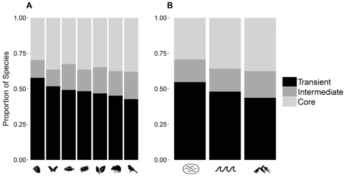
Assemblages from all ecosystem types and taxonomic groups included a substantial proportion of transient species, and relatively few species with intermediate temporal occupancy (Figure 2.3). The proportion of an assemblage made up of transient species varied with
16
transient, while birds had the lowest proportion of species classified as transients at 30%. Terrestrial ecosystems had the lowest proportion of transient species (37%) followed by marine (48%) and freshwater (55%) systems (Figure 2.3B).
There was a negative effect of sampling area on the proportion of transients in a community, but scaling relationships varied substantially in both slope and intercept across datasets and taxonomic groups (Figure 2.4A; simple R2 = 0.28, marginal R2 = 0.06). When we
characterized the scaling relationships using total community size based on the total number of individuals in an average sample instead of sample area the relationship was considerably stronger (Figure 2.4B; simple R2 = 0.43, marginal R2 = 0.12). Communities at scales in which
large numbers of individuals are sampled have few transient species, while communities at scales in which small numbers of individuals are sampled have proportionally more transient species, regardless of taxonomic group. After controlling for scale (community size), birds—one of the taxonomic groups with the lowest representation of transient species based on the raw survey data—became comparable to terrestrial invertebrates, which had the second highest
representation of transient species based on raw data (cf. Figure 2.3A and 4C). Mammal and plankton communities had the lowest average proportion of transient species in scale-corrected datasets at approximately 40%. Controlling for sampling scale, the proportion of transients in an assemblage no longer varied across type of ecosystem (Figure 2.4D). Elevational heterogeneity was found to have a positive effect (β = 0.023, t = 8.96, p < 10-16) on the proportion of transient
17
whereas assemblages excluding transient species were universally better fit by a lognormal distribution (Figure 2.5A). This shift to the lognormal was greater when excluding transient species compared to the null expectation generated by randomly excluding non-transient species (Appendix B). The strength of species richness drivers varied depending on whether transient species were included or not, because transient species exhibited environmental correlations of opposite sign to non-transient species (Figure 2.5B). As such, excluding transient species led to a stronger positive correlation between richness and the vegetation index NDVI, (0.52 versus 0.44), and a stronger negative correlation with mean elevation (-0.29 versus -0.07). Species turnover was always higher when transient species were included than when they were excluded, with an average deviation of 0.097 ± 0.166 (Figure 2.5C; see Figure A2.10 for similar results based on Bray-Curtis), and this deviation was greater compared to the null expectation from randomly excluding non-transient species (Appendix B). Finally, the exponent of the species-area relationship was typically higher when excluding transients (average deviation = 0.088 ± 0.114; Figure 2.5D). All results were similar using more conservative occupancy thresholds to define transient species (Figures A2.8-A2.9).
DISCUSSION
18
in distinct ways (Magurran and Henderson 2003, Ulrich and Ollik 2004, Coyle et al. 2013, Umaña et al. 2017), which highlights the need to better understand the contexts in which
transient species are expected to be prevalent and the potential impact transient species may have on ecological inferences.
The largest source of variation in the proportion of transient species observed in a community is related to spatial scale. For communities sampled at multiple spatial scales, the proportion of transient species decreased with increasing scale, as species were more likely to be observed and actually persist over larger sampling areas. While the scale-dependence of species richness is well understood (Rosenzweig 1995, Harte et al. 2009), the scale-dependence in the proportion of transient species within ecological assemblages is a newly described finding that has implications for the proper analysis of source-sink dynamics (Pulliam 1988; Amarasekare 2004) and metacommunity models (Leibold et al. 2004). If empirically the proportion of
transient species in an assemblage is high, then the scale at which that assemblage was measured is probably too small to represent a metacommunity patch with self-sustaining populations. The proportion of transient species in even larger regional assemblages potentially sheds light on the frequency of long distance, interregional dispersal events.
19
would have led to the conclusion that transient species were much more common in freshwater than terrestrial ecosystems.
Similarly, correcting for scale led to less variation in the distribution of the proportion of transient species across taxonomic groups (Figure 2.3C compared to 3A), and some groups that would have been inferred to differ substantially in the prevalence of transients were actually found to be comparable. Nevertheless, differences in the prevalence of transient species were evident among taxonomic groups even when controlling for spatial scale. Invertebrate, plant, and bird communities had the highest proportion of transient species while plankton and mammal communities had the lowest. While these taxonomic groups differ in many respects precluding a rigorous analysis, differences in traits related to dispersal ability and habitat specialization in particular are predicted by metacommunity theory (Leibold et al. 2004) to increase the likelihood of species being temporarily observed in areas where they are not well adapted and hence being recorded as transients. For example, birds have strong dispersal ability relative to the other taxonomic groups and there are numerous records of individuals spotted far outside their
geographic range and in unexpected habitats (Grinnell 1922). Similarly, plants with passive seed dispersal may be transported great distances and may consequently be more likely to be observed in unsuitable habitat (Willson 1993). Small mammals have more limited dispersal, which may explain why mammal communities (dominated in our dataset by small mammal communities) have a lower proportion of transient species on average. The plankton datasets examined in this study came primarily from lakes, and low rates of dispersal between lakes could explain the low proportion of transient species for this group.
20
populations in most locations. The low prevalence of transient species in plankton communities may also be explained by this phenomenon, as Hutchinson (1961) noted "paradoxically" that most plankton species are generalists that compete for the same limited resources. Specialist species, on the other hand, will only maintain populations in select locations with suitable conditions, allowing mass effects (Shmida and Wilson 1985, Leibold et al. 2004) or accidental dispersal to result in transient occurrences in other areas.
In addition to trait differences among taxa, variability in the prevalence of transient species was related to environmental heterogeneity. Transient species were more prevalent in communities with higher elevational heterogeneity, which extends the findings of Coyle et al. (2013) from birds to a broader range of taxa. Homogeneous landscapes tend to have
homogeneous communities (Stegen et al. 2013, Stein et al. 2014) and a site within such a landscape is unlikely to receive immigrants from poorly adapted species compared to a site in a heterogeneous landscape with a more diverse species pool from more diverse habitats. Indeed, environmental heterogeneity and species richness are frequently positively related (Stein et al. 2014), and our results indicate this may be due in part to an increase in transient species rather than an increase in habitat specialists (Gaston et al. 2007, Stein et al. 2014).
Impacts of Transient Species on Ecological Inference
21
distributions have been associated with different processes structuring the community (McGill et al. 2007, Connolly et al. 2014). Building on the results of Magurran and Henderson (2003), we show that including transient species—which typically occur at lower average abundance than non-transients—results in more logseries-like SADs while excluding them results in more lognormal distributions. This result is consistent with the idea that different processes influence the community assembly of transient versus core species (Henderson and Magurran 2014, Supp et al. 2015).
Should transient species be included in analyses of SADs? The answer will depend largely on the general framework and theories being tested. Based on theoretical grounds, many SAD models may be more appropriately applied to all species observed, or only to the set of species that strongly interact and maintain viable populations. For example, tests of neutral theory (Hubbell 2001) or metacommunity theory (Leibold et al. 2004) should include all species, as those theories explicitly allow for rare immigration events. In contrast, tests of resource allocation based niche apportionment models (MacArthur 1957, Tokeshi 1990)or purely niche based community assembly (Chase and Leibold 2003) are more appropriately applied only to assemblages of non-transient species which presumably exert stronger selection on each other. While the SAD may not be sufficient on its own to infer community structuring processes
(Cohen 1968, Volkov et al. 2005, Baldridge et al. 2016, Connolly et al. 2014), it is one of several ecological patterns that may collectively shed light on such mechanisms (McGill et al. 2007, Blonder et al. 2014). As such, consideration of transient species has the potential to influence our understanding of local community structure.
22
scale. Estimates of temporal turnover were always higher when transients were included in assemblages. This occurs because transient species are only present over a small fraction of a time series, resulting in higher turnover in species composition within a community over time (Magurran and Henderson 2010). Whether or not to include transient species in analyses involving temporal turnover depends on the question, and in some cases, the most useful information may result from analyzing the data both with and without transients. For example, when trying to understand how turnover relates to global change (Brown et al. 1997, Suding et al. 2008) we are likely interested in the influence on turnover in both groups, but since they are expected to be different and driven by different processes analyzing them separately will provide better inference.
While the inclusion of transient species inflated temporal turnover estimates, it led to lower estimates of spatial turnover as reflected in the slope of species-area relationships. This is because a greater proportion of the species list at small spatial scales are identified as transient compared to at a larger scale. As such, including transient species increases richness more at small scales than large, resulting in a shallower species-area relationship and lower spatial turnover (Figure 2.1D). For meta-analyses of the species-area relationship (Drakare et al. 2006), any of the factors that affect the proportion of transient species in an assemblage (scale,
23
indicating that consideration of transients is important for understanding local to regional scale ecological systems.
Finally, inclusion of transient species also influenced the strength of continental scale correlates of species richness. Excluding transient species increased the explanatory power of both NDVI and elevational heterogeneity. Transient species correlations were opposite of those observed for core species, consistent with our general findings on the relationships between environment and heterogeneity (Coyle et al. 2013). Because the proportion of transient species varies along environmental gradients, the perceived importance of environmental drivers of species richness and other ecological patterns may also change when excluding transient species. In this example, the inclusion of transients weakens the perceived support for a species-energy relationship (Wright 1983, Hurlbert 2004) compared to when only non-transients were
considered. Given the impact on a wide range of ecological patterns, the decision to include or exclude transient species in a community analysis is an important one that should be made by considering the nature of the conceptual framework or theory being investigated.
Metacommunity-like frameworks that explicitly consider low probability dispersal events between local sites are best evaluated using all species observed during sampling, but in many purely niche-based community assembly analyses, it will be necessary to remove transient species or risk making improper inferences.
Considerations
24
assemblage, much less across hundreds to thousands of sites across broad geographic extents. The bimodality of temporal occupancy distributions (e.g., Figure 2.1A) has led many authors to suggest that temporal occupancy can be used to distinguish these transient species from more core members of a community. However, it can sometimes be difficult to tease apart whether
species of low occupancy are truly transient or simply have low density or detectability (Henderson and Magurran 2014). We used a maximum occupancy threshold of 33% as our operational definition of transient species (Coyle et al. 2013), and the results we report here were similar using stricter thresholds of 10% or 25% (Figures C2.2-C2.6). If the focus were on a single community, then the accuracy of identifying transient species might be improved by a combination of assessing the shape and natural break points of each community's particular occupancy distribution, and incorporating information on species habitat preference as done by Belmaker (2009) for coral reef fish. Alternatively, when the sampling design allows for the estimation of detection probabilities it should be possible to correct for these issues using
occupancy modeling (MacKenzie et al. 2006). Independent validation of transient status (e.g., by evidence of breeding, or knowledge of habitat affinities) or occupancy modeling based
approaches should be considered when possible, and analyses along environmental gradients should carefully consider how detectability might vary along such gradients (Coyle et al. 2013). However, for many groups detailed information on habitat preferences or estimates of true population persistence is not readily available, and a definition based on a universal occupancy threshold is currently the most feasible option for analyzing hundreds or thousands of
assemblages for cross-taxon comparisons like those presented here.
25
Coyle et al. 2013). There is additional evidence from our results that using this raw occupancy based approach provides a reasonable approximate classification. First, the misclassification rate should presumably be lower when defining transient species using stricter occupancy thresholds, and so the consistency of our results across multiple thresholds lends some confidence to this approach. Second, for certain taxonomic groups and modes of data collection the assemblage data provide nearly complete censuses of all individuals within a static sample (e.g. plant stems within a quadrat or fish in a seine net). In these communities, imperfect detection should have little influence on estimates of occupancy (at the scale of sampling). The similarity of results in this study across groups that tend to be thoroughly surveyed (e.g., plants and fish) and those that are less intensively sampled (e.g., birds and butterflies) suggests that our results are not driven heavily by misclassifying imperfectly detected species. A detailed understanding of when and to what extent imperfect detection probabilities influence the assessment of the prevalence and impact of transient species will require simulation based approaches (Hurlbert unpublished data).
Conclusions
26
27 REFERENCES
Adler, P. B., E. P. White, W. K. Lauenroth, D. M. Kaufman, A. Rassweiler, and J. A. Rusak. 2005. Evidence for a General Species–Time–Area Relationship. Ecology 86:2032–2039. Azaele, S., A. Maritan, S. J. Cornell, S. Suweis, J. R. Banavar, D. Gabriel, and W. E. Kunin.
2015. Towards a unified descriptive theory for spatial ecology: predicting biodiversity patterns across spatial scales. Methods in Ecology and Evolution 6:324–332.
Baldridge, E., D. J. Harris, X. Xiao, and E. P. White. 2016. An extensive comparison of species-abundance distribution models. PeerJ 4:e2823.
Bates, D., M. Maechler, B. Bolker, and S. Walker (2015). Fitting Linear Mixed-Effects Models Using lme4. Journal of Statistical Software, 67(1), 1-48. doi:10.18637/jss.v067.i01. Belmaker, J. 2009. Species richness of resident and transient coral-dwelling fish responds
differentially to regional diversity. Global Ecology and Biogeography 18:426–436. Blonder, B., L. Sloat, B. J. Enquist, and B. McGill. 2014. Separating Macroecological Pattern
and Process: Comparing Ecological, Economic, and Geological Systems. PLOS ONE 9:e112850.
Bray, J. R., and J. T. Curtis. 1957. An Ordination of the Upland Forest Communities of Southern Wisconsin. Ecological Monographs 27:326–349.
Brown, J. H., T. J. Valone, and C. G. Curtin. 1997. Reorganization of an arid ecosystem in response to recent climate change. Proceedings of the National Academy of Sciences 94:9729–9733.
Chase, J. M., and M. A. Leibold. 2003. Ecological Niches: Linking Classical and Contemporary Approaches. Interspecific Interactions. First edition. University of Chicago Press.
Cohen, J. E. 1968. Alternate derivations of a species-abundance relation. The American Naturalist 102:165–172.
Connolly, S. R., M. A. MacNeil, M. J. Caley, N. Knowlton, E. Cripps, M. Hisano, L. M. Thibaut, B. D. Bhattacharya, L. Benedetti-Cecchi, R. E. Brainard, A. Brandt, F. Bulleri, K. E. Ellingsen, S. Kaiser, I. Kröncke, K. Linse, E. Maggi, T. D. O’Hara, L. Plaisance, G. C. B. Poore, S. K. Sarkar, K. K. Satpathy, U. Schückel, A. Williams, and R. S. Wilson. 2014. Commonness and rarity in the marine biosphere. Proceedings of the National Academy of Sciences 111:8524–8529.
28
Coyle, J. R., Hurlbert A. H., and E. P. White. 2013. Opposing Mechanisms Drive Richness Patterns of Core and Transient Bird Species. The American Naturalist 181:E83–E90. Dolan, J. R., M. E. Ritchie, A. Tunin-Ley, and M.-D. Pizay. 2009. Dynamics of core and
occasional species in the marine plankton: tintinnid ciliates in the north-west Mediterranean Sea. Journal of Biogeography 36:887–895.
Dornelas, M., N. J. Gotelli, B. McGill, H. Shimadzu, F. Moyes, C. Sievers, and A. E. Magurran. 2014. Assemblage Time Series Reveal Biodiversity Change but Not Systematic Loss. Science 344:296–299.
Drakare, S., J. J. Lennon, and H. Hillebrand. 2006. The imprint of the geographical, evolutionary and ecological context on species–area relationships. Ecology Letters 9:215–227.
Gaston, K. J., R. G. Davies, C. D. L. Orme, V. A. Olson, G. H. Thomas, T.-S. Ding, P. C. Rasmussen, J. J. Lennon, P. M. Bennett, I. P. F. Owens, and T. M. Blackburn. 2007. Spatial turnover in the global avifauna. Proceedings of the Royal Society of London B: Biological Sciences 274:1567–1574.
Gotelli, N. J., and R. K. Colwell. 2001. Quantifying biodiversity: procedures and pitfalls in the measurement and comparison of species richness - Gotelli - 2001 - Ecology Letters - Wiley Online Library.
Grinnell, J. 1922. The Role of The “Accidental.” The Auk 39:373–380.
Hanski, I., and M. Gyllenberg. 1993. Two General Metapopulation Models and the Core-Satellite Species Hypothesis. The American Naturalist 142:17–41.
Harte, J., A. B. Smith, and D. Storch. 2009. Biodiversity scales from plots to biomes with a universal species–area curve. Ecology Letters 12:789–797.
Henderson, P. A., and A. E. Magurran. 2014. Direct evidence that density-dependent regulation underpins the temporal stability of abundant species in a diverse animal community. Proc. R. Soc. B 281:20141336.
Hubbell, S. P. 2001. The Unified Neutral Theory of Biodiversity and Biogeography. http://press.princeton.edu/titles/7105.html.
Hurlbert, A. H. 2004. Species–energy relationships and habitat complexity in bird communities. Ecology Letters 7:714–720.
Hutchinson, G. E. 1961. The Paradox of the Plankton. The American Naturalist 95:137–145. Kitzes, J., and J. Harte. 2015. Predicting extinction debt from community patterns. Ecology
29
Krebs, C. 1999. Ecological Methodology. Second edition. Addison-Wesley Educational Publishers, Inc.
LaHuis, D. M., M. J. Hartman, S. Hakoyama, and P. C. Clark. 2014. Explained Variance Measures for Multilevel Models. Organizational Research Methods 17:433–451. Leibold, M. A., M. Holyoak, N. Mouquet, P. Amarasekare, J. M. Chase, M. F. Hoopes, R. D.
Holt, J. B. Shurin, R. Law, D. Tilman, M. Loreau, and A. Gonzalez. 2004. The metacommunity concept: a framework for multi-scale community ecology. Ecology Letters 7:601–613.
Luke, S. G. 2017. Evaluating significance in linear mixed-effects models in R | SpringerLink 49:1494–1502.
MacArthur, R. H. 1957. On the relative abundance of bird species. Proceedings of the National Academy of Sciences of the United States of America 43:293–295.
MacKenzie, D. I., J. D. Nichols, A. Royle, K. H. Pollock, L. L. Bailey, and J. E. Hines. 2006. Bimodal occupancy-frequency distributions uncover the importance of regional dynamics in shaping marine microbial biogeography | bioRxiv. Elsevier/Academic Press.
Magurran, A. E., and P. A. Henderson. 2003. Explaining the excess of rare species in natural species abundance distributions. Nature 422:714–716.
Magurran, A.E. and P.A. Henderson. 2010. Temporal turnover and the maintenance of diversity in ecological assemblages. Philosophical Transactions of the Royal Society of London B: Biological Sciences 365:3611–3620.
McGill, B. J., R. S. Etienne, J. S. Gray, D. Alonso, M. J. Anderson, H. K. Benecha, M. Dornelas, B. J. Enquist, J. L. Green, F. He, A. H. Hurlbert, A. E. Magurran, P. A. Marquet, B. A. Maurer, A. Ostling, C. U. Soykan, K. I. Ugland, and E. P. White. 2007. Species
abundance distributions: moving beyond single prediction theories to integration within an ecological framework. Ecology Letters 10:995–1015.
McGlinn, D. J., and M. W. Palmer. 2009. Modeling the sampling effect in the species-time-area relationship. Ecology 90:836–846.
Nakagawa, S., and H. Schielzeth. 2013. A general and simple method for obtaining R2 from generalized linear mixed-effects models. Methods in Ecology and Evolution 4:133–142. Novotný, V., and Y. Basset. 2000. Rare species in communities of tropical insect herbivores:
pondering the mystery of singletons. Oikos 89:564–572.
30
Pulliam, H. R. 1988. Sources, Sinks, and Population Regulation. The American Naturalist 132:652–661.
Rosenzweig, M. L. 1995. Species Diversity in Space and Time. Cambridge University Press. Shen, T.-J., and F. He. 2008. An Incidence-Based Richness Estimator for Quadrats Sampled
Without Replacement. Ecology 89:2052–2060.
Shmida, A., and M. V. Wilson. 1985. Biological Determinants of Species Diversity. Journal of Biogeography 12:1–20.
Southwood, T. R. E., V. C. Moran, and C. E. J. Kennedy. 1982. The Richness, Abundance and Biomass of the Arthropod Communities on Trees. Journal of Animal Ecology 51:635– 649.
Stegen, J. C., A. L. Freestone, T. O. Crist, M. J. Anderson, J. M. Chase, L. S. Comita, H. V. Cornell, K. F. Davies, S. P. Harrison, A. H. Hurlbert, B. D. Inouye, N. J. B. Kraft, J. A. Myers, N. J. Sanders, N. G. Swenson, and M. Vellend. 2013. Stochastic and deterministic drivers of spatial and temporal turnover in breeding bird communities. Global Ecology and Biogeography 22:202–212.
Stein, A., K. Gerstner, and H. Kreft. 2014. Environmental heterogeneity as a universal driver of species richness across taxa, biomes and spatial scales. Ecology Letters 17:866–880. Suding, K. N., S. Lavorel, F. S. Chapin, J. H. C. Cornelissen, S. Díaz, E. Garnier, D. Goldberg,
D. U. Hooper, S. T. Jackson, and M.-L. Navas. 2008. Scaling environmental change through the community-level: a trait-based response-and-effect framework for plants. Global Change Biology 14:1125–1140.
Supp, S. R., D. N. Koons, and S. K. M. Ernest. 2015. Using life history trade-offs to understand core-transient structuring of a small mammal community. Ecosphere 6:1–15.
Tokeshi, M. 1990. Niche Apportionment or Random Assortment: Species Abundance Patterns Revisited. Journal of Animal Ecology 59:1129–1146.
Ulrich, W., and M. Ollik. 2004. Frequent and occasional species and the shape of relative-abundance distributions. Diversity and Distributions 10:263–269.
Umaña, M. N., C. Zhang, M. Cao, L. Lin, and N. G. Swenson. 2017. A core-transient framework for trait-based community ecology: an example from a tropical tree seedling community. Ecology Letters 20:619–628.
31
White, A. E. 2016. Geographical Barriers and Dispersal Propensity Interact to Limit Range Expansions of Himalayan Birds. The American Naturalist 188:99–112.
White, E. P. 2004. Two-phase species–time relationships in North American land birds - White - 2004 - Ecology Letters - Wiley Online Library. Ecology Letters 7:329–336.
White, E. P., and A. H. Hurlbert. 2010. The Combined Influence of the Local Environment and Regional Enrichment on Bird Species Richness. The American Naturalist 175:E35–E43. Willson, M. F. 1993. Dispersal Mode, Seed Shadows, and Colonization Patterns. Vegetatio
107/108:260–280.
Wright, D. H. 1983. Species-Energy Theory: An Extension of Species-Area Theory. Oikos 41:496–506.
Xiao, X., E. P. White, M. B. Hooten, and S. L. Durham. 2011. On the use of log-transformation vs. nonlinear regression for analyzing biological power laws. Ecology 92:1887–1894. Yenni, G., P. Adler, and M. Ernest. 2016. Do persistent rare species experience stronger negative
32
Figure 2.1. (A) Bimodal distribution of temporal occupancy for North American birds from Coyle et al. (2013) illustrating one mode of "core" species observed consistently at sites and a mode of low occupancy "transient" species observed irregularly. (B) Core and transient species exhibit different species abundance distributions for the Hinkley Point fish assemblage
(Magurran and Henderson 2003). (C) Four contiguous quadrats in which species (different shapes) may be core (shaded) or transient (open). (D) The species-area relationships for (C) depending on whether transient species are excluded or not, using the lower right panel to
represent the smallest area. Because every species is core in at least one quadrat, species richness at the largest scale is the same for the two relationships. (E) Temporal turnover (the Jaccard
log(area) log (S pe ci es
) All species
Exclud ing tra
nsient s
B
A
C
D
Transient Coretime !!
All species:
E
time !"
Excluding
transients: 0 = 0%
= 50%
33
index of dissimilarity) is much lower when transient species are excluded from the calculation, since they are the species most driving turnover.
Figure 2.2. Description of the compiled time-series datasets. The number of (A) datasets and (B) number of assemblages (log scaled) by ecosystem type (terrestrial, freshwater, marine) and by taxonomic group (C, D). (E) Boxplots of the number of species per assemblage by taxonomic group. (F) Boxplots of time series length by taxonomic group.
Birds
Plants
Mammals Fish
Invertebrates Benthos Plankton Terrestrial
34
35
Figure 2.4. Linear models of the proportion of transient species as a function of (A) sample area and (B) sample community size (summed abundance across all species) for each dataset with a spatially hierarchical sampling scheme. Datasets are color coded by taxonomic group and a solid black line represents the fit for all data. The proportion of transient species expected for a
hypothetical community of 102 individuals fitted to the linear model used in Figure 2.4B (the dotted vertical line represents the median community size across datasets) for a given (C) taxonomic group or (D) ecosystem based on linear mixed effects models (see text) using predicted values. Error bars represent the upper and lower limits of the 95% prediction interval from the predictInterval command of the merTools R package. No spatially hierarchical datasets were available to evaluate benthic invertebrates. See Figure 2.2 for icon key.
Simple R2 = 0.29 Marginal R2 = 0.01
36
Figure 2.5. Comparison of common ecological patterns between full communities and communities excluding transient species. (A) Histogram of Akaike weights for the logseries model of the species abundance distribution for all species (orange) and excluding transients (yellow); areas of overlap are in light orange. Because only two models were compared, Akaike weights close to 0 imply strong support for the lognormal model. (B) Environmental correlates of species richness (NDVI and elevation) including transients (orange), excluding transients (yellow), and transients only (pink). (C) Comparison of temporal turnover estimates when including or excluding transient species. Temporal turnover was quantified using the Jaccard dissimilarity index. Points are color coded by taxa and small blue circles represent the North American Breeding Bird Survey. (D) Comparison of species-area relationship exponents when including or excluding transient species. Points are the same as in (C).
0.5 0
37
CHAPTER 3: THE RELATIVE IMPORTANCE OF BIOTIC AND ABIOTIC DETERMINANTS OF TEMPORAL OCCUPANCY FOR AVIAN SPECIES IN NORTH
AMERICA
INTRODUCTION
38
traditional measures for describing species distributions, although any interpretations of observed temporal occupancy values must consider how detectability might vary across species and
environments to influence such patterns.
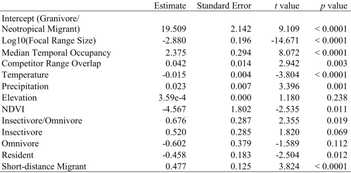
Generally, species require specific environmental conditions to succeed in a particular habitat, but often they do not occur everywhere the environment is suitable (Hutchinson 1957; Chesson 2000a, Gaston 2003). This distinction between the fundamental and realized niche is usually ascribed to interspecific interactions, such as where a species is outcompeted in parts of its suitable range by a superior competitor (Arif, Adams, & Wicknick, 2007; Connell, 1961; Cunningham, Rissler, Buckley, & Urban, 2016). Recent studies have demonstrated that including both positive and negative interspecific interactions can lead to more complete and accurate species distribution models (Belmaker et al., 2015; Blois, Zarnetske, Fitzpatrick, & Finnegan, 2013; Bruno, Stachowicz, & Bertness, 2003; Gotelli, Graves, & Rahbek, 2010; Guisan & Thuiller, 2005; Wisz et al., 2013). Interspecific competition for desirable habitat and resources may be the most relevant biotic interaction at large temporal and spatial scales of study and is the most studied biotic interaction for shaping species ranges (Sexton, McIntyre, Angert, & Rice, 2009). While many have argued for considering both environmental conditions and biotic factors in order to fully explain species’ distributions, there is not yet consensus on the relative
importance of these two categories of drivers, or on the types of species traits that might influence that relative importance.
39
temporal occupancy than abundance. We also examine whether species migratory and foraging traits can help explain why temporal occupancy is better predicted by abiotic variables for some species and biotic interactions for others.
METHODS Bird data
Birds are particularly suitable for modeling species ranges since they are well-studied and there is ample data on their presence over time at large spatial extents (Bennett, Clarke,
40 Biotic drivers
For each focal species, competitor species were identified as those species in the same
family with any area of overlapping geographic range and within a two-fold range of body mass (Dunning, 2007). These criteria are commonly used indicators of potential competitive
interactions in birds (Dhondt, 2012; Elsen, Tingley, Kalyanaraman, Ramesh, & Wilcove, 2017; Price, 1991; Yackulic, 2017). A comprehensive list of focal and associated competitor species is included in online supplemental material
(https://onlinelibrary.wiley.com/doi/full/10.1111/geb.13064). In some cases, potential
competitors from outside the focal species’ family were included when such interactions were specifically described in natural history accounts (e.g. American Redstart, Setophaga ruticilla and Least Flycatcher, Empidonax minimus, Sherry 1979). For each focal species, the competitor with the greatest percentage of breeding range overlap was also identified (hereafter, the most widespread competitor) based on BirdLife International shapefiles.
At each survey route r, we calculated an index of overall competitive pressure based on the summed abundance of all potential competitors relative to the focal species
𝑐!"#,% = ∑ '(,)
∑ '(,)*'+,) (1)
where ni,r and nj,r are the abundances of focal species i and the jth competitor of species i,