A MONTE CARLO METHOD TO ESTIMATE RADIATION DOSE FROM CONE BEAM COMPUTED TOMOGRAPHY
Jacob S. Dunn
A thesis submitted to the faculty at the University of North Carolina at Chapel Hill in partial fulfillment of the requirements for the degree of Master of Science in the
School of Dentistry (Oral and Maxillofacial Radiology).
Chapel Hill 2015
ABSTRACT
Jacob S. Dunn: A Monte Carlo method to estimate radiation dose from cone beam computed tomography
(Under the direction of John B. Ludlow)
Objectives: This study compares effective dose determination of four large field of view CBCT units (NewTom-3G, Galileos Comfort Plus, CS-9300, iCat-FLX,) using a Monte Carlo software analysis method (PCXMC) and dosimetry using anthropomorphic phantoms.
Methods: Previous research provided phantom effective dose comparisons. Field-of-view and phantom positioning were duplicated in the software. Software and phantom dosimetry values were compared. Descriptive statistics, chi-square, and logistic regression, were used to analyze the data. The null-hypothesis that there is no statistically significant difference between the dosimetry values of the anthropomorphic phantom and the calculated values of the PCXMC software was tested.
Results: PCXMC simulated scans produced dose values within 20% of the phantom dosimetry 48-58% of the time.
ACKNOWLEDGEMENTS
I would like to express my sincere appreciation for my mentor and committee for their unyielding support, and particularly for their ability (and faith) to operate from 10,000 feet.
TABLE OF CONTENTS
LIST OF TABLES ... vii
LIST OF FIGURES ... viii
LIST OF ABBREVIATIONS AND SYMBOLS ... ix
DEVELOPMENT OF MONTE CARLO ... 1
The Monte Carlo Method ... 2
THE USE OF MONTE CARLO WITH DENTAL CBCT: REVIEW OF LITERATURE ... 4
Monte Carlo Programs in Dentistry ... 4
Monte Carlo Programs and Dental CBCT ... 6
PCXMC Studies in the Literature ... 8
BACKGROUND ... 9
OBJECTIVES ... 12
MATERIALS AND METHODS ... 13
RESULTS ... 22
DISCUSSION ... 29
Limitations ... 30
PCXMC Previous Validation Studies ... 32
Organ doses ... 33
Future Directions... 35
CONCLUSIONS ... 36
APPENDIX 1: MAS INPUT VARIABLE ORGAN CHI-SQUARE ANALYSIS ... 37
APPENDIX 2: DAP INPUT VARIABLE ORGAN CHI-SQUARE ANALYSIS ... 41
LIST OF TABLES
Table 1: NewTom 3G Included Image Protocol ... 13
Table 2: Galileos Comfort Plus Included Image Protocols ... 14
Table 3: CS9300 Included Image Protocols ... 15
Table 4: iCat FLX Included Image Protocols ... 16
LIST OF FIGURES
Figure 1: PCXMC angle orientation relative to patient (As if looking up through the floor, so
patient left is 0 degrees) ... 18
Figure 2: PCXMC Positioning and scout window ... 19
Figure 3: NewTom 3G PCXMC effective dose estimates relative to phantom ... 22
Figure 4: Sirona Galileos Comfort Plus PCXMC effective dose estimates relative to phantom ... 23
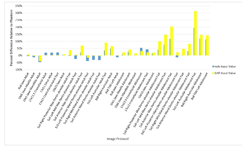
Figure 5: CS9300 PCXMC effective dose estimates relative to phantom... 24
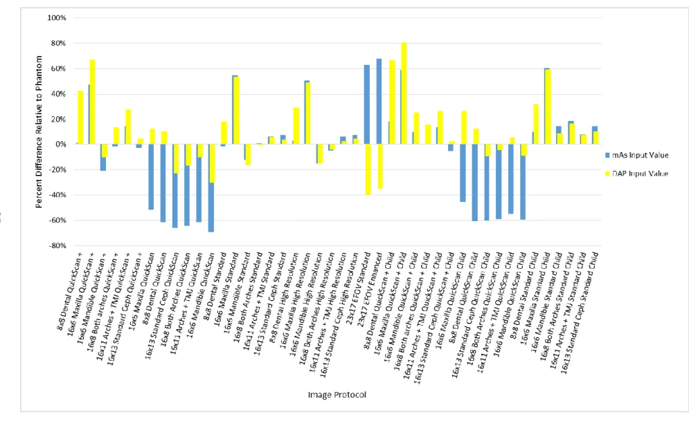
Figure 6: iCat FLX PCXMC effective dose estimates relative to phantom ... 25
Figure 7: Logistic Regression with mAs as the input variable. Variables examined included machine used, phantom used (adult or child), FOV location, FOV volume size, and phantom measured dose ... 26
Figure 8: Logistic Regression with DAP as the input variable. Variables examined included machine used, phantom used (adult or child), FOV location, FOV volume size, and phantom measured dose. ... 27
Figure 9: Percentage of PCXMC organ dose estimates within ±20% of phantom, with DAP or mAs as input variable. ... 27
Figure 10: Chi-square standardized residuals, with mAs as input value ... 28
Figure 11: Chi-square standardized residuals, with DAP as input value ... 28
LIST OF ABBREVIATIONS AND SYMBOLS
BREP Boundary representation (phantom) CBCT Cone beam computed tomography
DAP Dose area product
ENIAC Electronic Numerical Integrator and Computer
FOV Field of View
ICRP International Commission on Radiological Protection LANL Los Alamos National Laboratory
MC Monte Carlo
MDCT Multi-detector computed tomography MIRD Medical Internal Radiation Dose
MOSFET Metal-oxide-semiconductor field-effect transistor
MR Magnetic Resonance
NCRP National Council on Radiation Protection and Measurements ORNL Oak Ridge National Laboratory
OSLD Optically stimulated luminescent dosimeter RANDO Radiation analog dosimetry system
SID Source to image distance
SMV Submentovertex
TLD Thermoluminescent dosimeter
TMJ Temporomandibular joint
VCH Visible Chinese Human
Π The numerical value of the ratio of the circumference of a circle to its diameter. NOT made of cherry. Although a whole pie CAN be used to calculate π. Read on to find out!
DEVELOPMENT OF MONTE CARLO
“The first thoughts and attempts I made to practice [the Monte Carlo method] were suggested by a question which occurred to me in 1946 as I was convalescing from an illness and playing solitaires. The question was what are the chances that a Canfield solitaire laid out with 52 cards will come out successfully? After spending a lot of time trying to estimate them by pure combinatorial calculations, I wondered whether a more practical method than “abstract thinking” might not be to lay it out say one hundred times and simply observe and count the number of successful plays. This was already possible to envisage with the beginning of the new era of fast computers, and I immediately thought of problems of neutron diffusion and other questions of mathematical physics, and more generally how to change processes described by certain differential equations into an equivalent form interpretable as a succession of random operations.”1
These remarks were made by Stanislaw Marcin Ulam, a Polish-American scientist who was one of the primary contributors in the development of the Monte Carlo method. Born in 1909 Lviv, in a Polish area of now Ukraine that was then part of the Austro-Hungarian Empire, Ulam studied mathematics throughout Europe until he was invited in 1935 to come to the Institute for Advanced Study in Princeton, New Jersey.2 This led to opportunities for research at Harvard University in Cambridge, Massachusetts, until he became an assistant professor at the University of Wisconsin-Madison.2
had been working out calculations on the first general electronic computer, called the Electronic Numerical Integrator and Computer (ENIAC).4 While Ulam was reviewing these calculations, he realized that the faster calculating ability of this machine would allow the reality of a method of statistical analysis he had considered while playing solitaire during a previous convalescence.1 Von Neumann applied Ulam’s thought to a proposal to evaluate the behavior of neutrons during nuclear fission.5 Metropolis code named it “The Monte Carlo method” because Ulam had mentioned an uncle who frequented the Monte Carlo casinos.4 Together, they published an early, unclassified paper on the subject.6
The Monte Carlo Method
The Monte Carlo (MC) method is a statistical approach to solving problems in systems in which there is a degree of uncertainty. There are many methods to accomplish the task, but basic points include the following: the definition of the domain of possible inputs, the
generation of random inputs based on probability actions within that domain, the computation of results (calculating a successful ‘hit’ or not, based on the definition of the domain), and finally an aggregation of the results.7 A simple example of this would be an attempt to calculate the value of π. If a circle is circumscribed within a square and drawn on the floor, the ratio of the areas (circle to square) is π/4. If many, many pins were dropped at random within the entirety of the square, and counted at the end, the number of points within the circle relative to the entirety of the square would also be very close to the fraction, π/4.7 This is one basic example of using the Monte Carlo method, including the inherent random sampling, to solve a
mathematical problem.
of internal structures (organs) and characteristics of the organs (volume, shape, and attenuation). The distribution of the photons utilize both measurements and theoretical properties of x-rays.7 Kalos and Whitlock effectively describe the steps involved:
1. Pick a set of source variables (initial state of system). 2. Follow the x-ray until it interacts with an atom. 3. Determine whether the x-ray scatters
-if so, repeat from step 2; -if not, terminate the history.
Steps 2 and 3 are repeated until the x-ray photon is absorbed or is no longer capable of effecting the answer to any appreciable extent.
4. Repeat the whole process from step 1 as many times as necessary to achieve the accuracy needed for the solution.
5. Take arithmetic average of answers of all the histories.7
This sequence describing radiation transport in a system is essentially a “random walk” or a Markov chain, a process that has stepwise transitions involving randomness and
probability.9, 10 Each step is a collision event, which outcome depends on the characteristics of the radiation and interaction medium. Modeling of these collisions requires listing the possible events, then assigning the probability of each of those events occurring. Just like with
Hollywood actors, the life history of the photon is closely followed until interest in it is lost or it is terminated.7 Interest is lost when the photon is too low in energy to affect the answer, and termination occurs with a photoelectric effect or when it exits the system. To summarize, the process simulates an x-ray photon with “random position, direction, and time, which travels in straight-line segments whose lengths are random; the photon interacts with the atoms
THE USE OF MONTE CARLO WITH DENTAL CBCT: REVIEW OF LITERATURE
A search for the term ‘monte carlo’ on PubMed yields nearly 40,000 results, illustrating the near ubiquity of this technique within medical physics, physical sciences, engineering, computer science, applied statistics, mathematics, artificial intelligence, image processing, biology, and even finance and business.11, 12
A review of the literature was completed on PubMed with the assistance of the School of Dentistry librarian. The search used the terms “cone beam computed tomography AND
dosimetry AND ‘monte carlo’”, and “cone beam computed tomography AND dosimetry AND ‘monte carlo’ AND (dentistry OR dental)”, and “‘monte carlo’ AND (dentistry OR dental)”.
The majority of the articles involving cone beam computed tomography (CBCT) and Monte Carlo (MC) programs evaluate dose characteristics of the onboard CBCT as part of a linear accelerator used in image guided radiation therapy (IGRT).13-43 Additionally, dose
evaluations of the associated electronic portal imaging devices are also common.16, 21, 44-46 Other studies involve dose evaluation of multi-detector computed tomography (MDCT),47-57 mega voltage CT,58-61 medical CBCT involving neurology,62 fluoroscopy,63 angiography,64
mammography,65-67 and evaluation of internal radionuclides.68, 69 Of image quality interest are articles that evaluate CBCT scatter with the goal of image quality improvement through scatter reduction.70-72
Monte Carlo Programs in Dentistry
dose when adding rare earth filters,78 the electron paramagnetic resonance as a measure of dose within enamel,79 enamel beam hardening in micro CT,80 variations in light-induced fluorescence in enamel in the presence of caries,81 maxillofacial fluoroscopy82, and even estimates of caries in extended populations in Australia83.
Several studies use Monte Carlo methods to evaluate dose with dental plain film
radiography. Aps and co-workers investigated lateral radiographs and bitewing radiographs.84 Batista and co-workers looked at the dose in panoramic images from conventional and CBCT machines.85 Lee and co-workers (2012) studied the effect of collimation in cephalography.86 Nicopoulou-Karayianni and co-workers looked at radiation absorbed doses at titanium-bone interfaces in diagnostic dental radiography.87 Walker and co-workers proposed diagnostic references levels for intraoral and panoramic radiography.88
Dr. Julian Gibbs led several studies at Vanderbilt University involving Monte Carlo analysis and dental radiography.89-93 In 1982, Gibbs created a MC method to evaluate the dose distribution of an 80 kVp x-ray beam on a homogenous water phantom. He found no significant differences between the estimated doses and the doses measured with an ionization chamber. In 1984, he used the same MC program to evaluate dose from molar interproximal radiographs on a voxel CT phantom of an adult female cadaver. The voxels within the phantom were coded as air, lung, fat, muscle bone, or tooth, with attenuation factors coinciding with the then
contemporary ICRP Reference Man recommendations. X-rays were programmed to operate at 90 kVp. The sequence was run with a target-skin distance of 20 cm with round collimation, and 40 cm with rectangular collimation. Gibbs found that the use of long-cone technique with rectangular collimation would reduce the cancer risk by a factor of 2.9.90
In 1987, Gibbs and co-workers used the same MC program and same female cadaver phantom to evaluate the dose to sensitive organs during intraoral radiography. The
female cadaver phantom, Gibbs and co-workers simulated three radiographic examinations: chest, dental full mouth series, and dental panoramic. The investigators found that collimated dental examinations, while being less homogenous than the chest examination, concentrated dose to organs of the head and neck.92
In 2000, Gibbs used the same MC program and cadaver phantom to evaluate additional radiographic protocols, including submentovertex (SMV), temporomandibular joint (TMJ), cephalometric, and a chest PA and lateral images. Organ doses for each projection were
determined at 70, 80, and 90 kVp. Gibbs found that effective dose and effective dose equivalent calculations varied significantly between organs, depending on image protocol.93
Monte Carlo Programs and Dental CBCT
Fully six articles deal with dosimetry using Monte Carlo methods on dental CBCT.94-99 In 2010, Vassileva and co-workers used PCXMC (STUK, Helsinki, Finland) to estimate effective dose of the ILUMA Ultra CBCT (IMTEC Imaging, Ardmore, OK). Software estimated effective doses were lower than those calculated with RANDO (The Phantom Laboratory, Salem, NY) phantom dosimetry by Ludlow and Ivanovic by over 68% with ICRP 103 recommendations.97, 100
In 2011, Zhang and co-workers evaluated the 3D Accuitomo 170 unit (J Morita, Japan), using the BEAMnrc/EGSnrc MC code system to simulate x-ray generation, filtration, and collimation. Kerma free-in-air at the isocenter was validated by comparison against measured air kerma in water in a cylindrical water phantom. Discrepancies between the two
cm. For the Scanora, a 14.5x7.5 cm, 10x7.5 cm, and 6x6 cm FOV was included. Absorbed organ dose and effective dose were calculated. Of note is the fact that the thyroid was not part of the head/neck of any of the four phantoms, and as such, it was not included in the calculation of effective dose.99 The authors found that organ dose varied as much as 112% between phantoms, and that between the two machines examined, variation of organ doses between phantoms was greater than dose differences between machines. Effective dose varied up to 30% (in terms of coefficient of variation, defined as the ratio of standard deviation to the mean, expressed as a percentage). Differences in phantom anatomy were was surmised as the reasoning behind the difference in effective dose.
In 2012, Koivisto and co-workers evaluated effective dose on the Promax 3D CBCT (Planmeca, Helsinki, Finland) using new metal-oxide semiconductor field-effect transistors (MOSFET) dosimeter devices, and compared them with PCXMC estimated results. The dosimeters were placed in a RANDO phantom according to protocol described by Ludlow and co-workers.101 The field of view (FOV) was 8x8cm, and positioned to capture the oral cavity volume. The phantom scans and simulations were performed at various heights on the z-axis, to evaluate vertical positioning on effective dose. Both the phantom and the simulation noted a distinct relationship between the presence of the thyroid within the scan, (and accordingly that organ’s equivalent dose) and total effective dose. The difference between MOSFET measured and PCXMC estimated effective dose differed by as much as 52%, and differences in individual organ equivalent doses varied as much as 600%.102 Differences between the two were equated to differences in the mathematically modeled and physical phantom, regarding shape, volume, and positioning of the organs, particularly the thyroid. Additionally, the authors noted that small differences in phantom head position had a substantial effect on effective dose.102
chamber measurements and thermoluminescent dosimeters (TLD) in a water-filled Remab male adult phantom (Alderson Research Laboratory). The imaging protocols examined were the “Landscape 13cm” and “Extended Field of View (Cephalometric, E-FOV)”. Within the ionization chambers, percent difference between the two methods ranged up to 6%. Within the phantom, relative differences between the organ dose values (mGy to air) ranged 1-84%, although more than half had less than 13% difference. Statistical uncertainties of the MC program ranged 7-19% for dose values ≥1 mGy, and increased to 100-130% for values of 0.01 mGy.95
Morant and co-workers again in 2013 studied MC program EGS4 simulated doses on the iCat next-generation CBCT. The ICRP voxel adult male and female reference phantoms (AM and AF) were evaluated. Nine different FOVs were simulated. The authors found that organ and effective dose varied according to FOV, beam acquisition angles and positioning. The full head scan (23 x 17cm FOV) estimated effective dose was 47% less than the results of Ludlow and Ivanovic, however, Davies and co-workers showed reasonable agreement with the other imaging protocols.100, 103
PCXMC Studies in the Literature
A review of the literature was completed on PubMed with the search term “PCXMC.” Aside from the studies mentioned previously, the majority of studies involved radiography within the pediatric community.104-126 Other studies included fluoroscopy,127-133 angiography,134, 135 other interventional radiography,136-139 tomosynthesis,140-143 and CBCT as a part of image guided radiation therapy.144-146 On the more technical side, studies investigated dose relating to structural shielding,147 source-to-image distance (SID),148, 149 dose-area-product (DAP),150
BACKGROUND
Shortly after the initial discovery of x-rays by Wilhelm Roentgen, dentistry began incorporating radiology as a means of diagnosis.155 Through the years, the technology and use has kept pace with the increasing range and variation of treatment. The utilization of radiology in dentistry was expanded with the development of commercial panoramic tomography in the early 1960s.156 The parallel development of cone beam computed tomography (CBCT), although nearly thirty years later, also allowed new avenues and diagnostic abilities.157
The use of CBCT imaging has significantly increased within general dentistry,
endodontics, oral surgery, periodontics, and orthodontics.158-165 This increasing popularity of this technology is understandable with the ability of CBCT to reconstruct volumes, as well as present multi-planar simultaneous views, enabling the dental practitioner potentially much more information than previous two-dimensional radiography. Responding to the demand within the field, there are currently many firms that manufacture CBCT machines, with multiple models often produced within each company.166
radiation exposure from CBCT is usually lower than from CT, it is important to understand that risks of exposure still exist and that imaging principle of exposure parameters as low as
reasonably achievable (ALARA) still applies to CBCT examination protocols.171, 172
With ionizing radiation, concern exists with both deterministic effects of radiation, those effects produced above a certain threshold dose, and stochastic effects, those effects that are random and probabilistic.168, 173 With CBCT dose levels, the primary concern is with stochastic effects. Since limited data exists on radiation exposure and sequelae with small doses,
extrapolation is required from higher dose evaluation.168 A fundamental problem is that different CBCT units have different doses for similar exam protocols, and there is no
standardization of dose for a specific image.165 Accurate machine specific dosimetry is vital. The current standard for dosimetry incorporates anthropomorphic phantoms, those commonly used include the radiation analog dosimetry system (RANDO) phantom (The Phantom Laboratory, Salem, NY), ATOM phantom (CIRS, Norfolk, VA), as well as a several others.165, 174-185 This standard is time-consuming, costly, and technique sensitive.186 A simple, inexpensive, and accurate method needs to be developed to measure dose and assess risk for a given scan.
The parallel quest in medicine to develop effective and inexpensive dosimetry has led to mathematical software analysis. One such software analysis method, named Monte Carlo, has become prevalent. The development actually began with the research in the 1940s on radiation shielding for the Manhattan Project.12 Although the specific physical parameters of the project were known, the solutions were eluding the researchers using traditional mathematical
OBJECTIVES
This study compared effective dose determination of four large field of view CBCT units (CS-9300, NewTom-3G, iCat-FLX, and Galileos Comfort Plus) using a specific Monte Carlo software analysis method, PCXMC 2.0 (STUK, Helsinki, Finland), developed by Tapiovaara and co-workers for the Finnish Radiation Nuclear Safety Authority and dosimetry using
anthropomorphic phantoms. The program uses a mathematically determined computational phantom. That information was used with the 2007 Tissue Weight factors from the ICRP to calculate the effective dose.
As accurate dosimetry is an important step in minimizing patient risk during radiologic examinations, accurate methods are needed to assess that risk. Within medicine, dosimetry has advanced significantly, and Monte Carlo methods are widely used. The goal of this study is to extend verification of Monte Carlo methods to additional dental CBCT units, and compare the accuracy of this specific software analysis methodology with dental dosimetry using
MATERIALS AND METHODS
This study compares simulated effective dose results from PCXMC, a user friendly, commercially available Monte Carlo method software application, with the effective dose results from previous research using dosimeters placed in tissue equivalent anthropomorphic
phantoms. The previous research was completed by Ludlow and co-workers evaluating the NewTom 3G (Cefla Dental Group, Imola, IT) using a RANDO phantom and thermoluminescent dosimeters (TLDs), and the Galileos Comfort Plus HD (Sirona Dental Systems, Inc. Long Island City, NY), the CS 9300 (Carestream Dental, Atlanta, USA) and the iCat FLX (Imaging Sciences International, Hatfield, PA) using ATOM phantoms and optically stimulated dosimeters
(OSLDs).100, 101, 165, 192 Differences between the use of OSLs and TLDs, and the use of ATOM and RANDO phantoms were found to be less than 2% in the calculations of effective dose with ICRP 103 values.192 Table 1Table4 show the imaging protocols that were used on the physical
phantoms for each machine. These protocols were duplicated in the PCXMC software, using the input parameters listed in table 5.
Table 1: NewTom 3G Included Image Protocol
Full 30 x 30
Adult
8.1
362.2
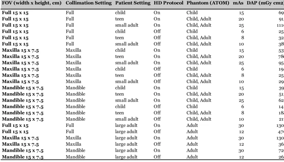
Table 2: Galileos Comfort Plus Included Image Protocols
Full 15 x 15 Full child On Child 15 697
Full 15 x 15 Full teen On Child, Adult 20 915
Full 15 x 15 Full small adult On Child, Adult 25 1110
Full 15 x 15 Full child Off Child 6 252
Full 15 x 15 Full teen Off Child, Adult 8 328
Full 15 x 15 Full small adult Off Child, Adult 10 387
Maxilla 15 x 7.5 Maxilla child On Child 15 537
Maxilla 15 x 7.5 Maxilla teen On Child, Adult 20 780
Maxilla 15 x 7.5 Maxilla small adult On Child, Adult 25 958
Maxilla 15 x 7.5 Maxilla child Off Child 6 194
Maxilla 15 x 7.5 Maxilla teen Off Child, Adult 8 252
Maxilla 15 x 7.5 Maxilla small adult Off Child, Adult 10 298
Mandible 15 x 7.5 Mandible child On Child 15 391
Mandible 15 x 7.5 Mandible teen On Child, Adult 20 513
Mandible 15 x 7.5 Mandible small adult On Child, Adult 25 622
Mandible 15 x 7.5 Mandible child Off Child 6 142
Mandible 15 x 7.5 Mandible teen Off Child, Adult 8 184
Mandible 15 x 7.5 Mandible small adult Off Child, Adult 10 217
Full 15 x 15 Full large adult On Adult 30 1301
Full 15 x 15 Full large adult Off Adult 12 470
Maxilla 15 x 7.5 Maxilla large adult On Adult 30 1301
Maxilla 15 x 7.5 Maxilla large adult Off Adult 12 362
Mandible 15 x 7.5 Mandible large adult On Adult 30 729
Mandible 15 x 7.5 Mandible large adult Off Adult 12 263
mAs DAP (mGy cm2) FOV (width x height, cm) Collimation Setting Patient Setting HD Protocol Phantom (ATOM)
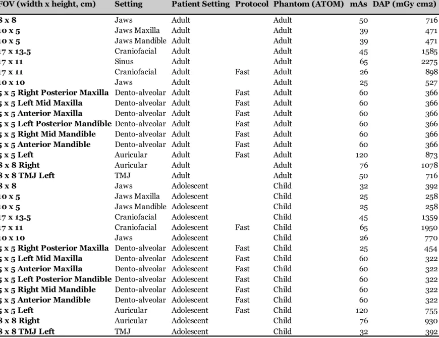
Table 3: CS9300 Included Image Protocols
8 x 8 Jaws Adult Adult 50 716
10 x 5 Jaws Maxilla Adult Adult 39 471
10 x 5 Jaws Mandible Adult Adult 39 471
17 x 13.5 Craniofacial Adult Adult 45 1585
17 x 11 Sinus Adult Adult 65 2275
17 x 11 Craniofacial Adult Fast Adult 26 898
10 x 10 Jaws Adult Adult 25 527
5 x 5 Right Posterior Maxilla Dento-alveolar Adult Fast Adult 60 366
5 x 5 Left Mid Maxilla Dento-alveolar Adult Fast Adult 60 366
5 x 5 Anterior Maxilla Dento-alveolar Adult Fast Adult 60 366
5 x 5 Left Posterior MandibleDento-alveolar Adult Fast Adult 60 366
5 x 5 Right Mid Mandible Dento-alveolar Adult Fast Adult 60 366
5 x 5 Anterior Mandible Dento-alveolar Adult Fast Adult 60 366
5 x 5 Left Auricular Adult Fast Adult 120 873
8 x 8 Right Auricular Adult Adult 76 1078
8 x 8 TMJ Left TMJ Adult Adult 50 716
8 x 8 Jaws Adolescent Child 32 392
10 x 5 Jaws Maxilla Adolescent Child 25 258
10 x 5 Jaws Mandible Adolescent Child 25 258
17 x 13.5 Craniofacial Adolescent Child 45 1359
17 x 11 Craniofacial Adolescent Fast Child 65 1950
10 x 10 Jaws Adolescent Child 26 770
5 x 5 Right Posterior Maxilla Dento-alveolar Adolescent Fast Child 25 454
5 x 5 Left Mid Maxilla Dento-alveolar Adolescent Fast Child 60 322
5 x 5 Anterior Maxilla Dento-alveolar Adolescent Fast Child 60 322
5 x 5 Left Posterior MandibleDento-alveolar Adolescent Fast Child 60 322
5 x 5 Right Mid Mandible Dento-alveolar Adolescent Fast Child 60 322
5 x 5 Anterior Mandible Dento-alveolar Adolescent Fast Child 60 322
5 x 5 Left Auricular Adolescent Fast Child 120 755
8 x 8 Right Auricular Adolescent Child 76 930
mAs DAP (mGy cm2) FOV (width x height, cm) Setting Patient Setting Protocol Phantom (ATOM)
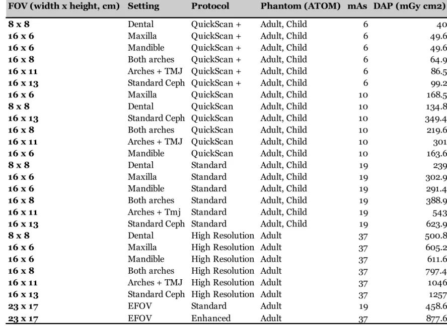
Table 4: iCat FLX Included Image Protocols
8 x 8
Dental
QuickScan +
Adult, Child
6
40
16 x 6
Maxilla
QuickScan +
Adult, Child
6
49.6
16 x 6
Mandible
QuickScan +
Adult, Child
6
49.6
16 x 8
Both arches
QuickScan +
Adult, Child
6
64.9
16 x 11
Arches + TMJ QuickScan +
Adult, Child
6
86.5
16 x 13
Standard Ceph QuickScan +
Adult, Child
6
99.2
16 x 6
Maxilla
QuickScan
Adult, Child
10
168.5
8 x 8
Dental
QuickScan
Adult, Child
10
134.8
16 x 13
Standard Ceph QuickScan
Adult, Child
10
349.4
16 x 8
Both arches
QuickScan
Adult, Child
10
219.6
16 x 11
Arches + TMJ QuickScan
Adult, Child
10
301
16 x 6
Mandible
QuickScan
Adult, Child
10
163.6
8 x 8
Dental
Standard
Adult, Child
19
239
16 x 6
Maxilla
Standard
Adult, Child
19
302.9
16 x 6
Mandible
Standard
Adult, Child
19
291.4
16 x 8
Both arches
Standard
Adult, Child
19
388.9
16 x 11
Arches + Tmj
Standard
Adult, Child
19
543
16 x 13
Standard Ceph Standard
Adult, Child
19
623.9
8 x 8
Dental
High Resolution Adult
37
500.8
16 x 6
Maxilla
High Resolution Adult
37
605.2
16 x 6
Mandible
High Resolution Adult
37
611.6
16 x 8
Both arches
High Resolution Adult
37
797.4
16 x 11
Arches + TMJ High Resolution Adult
37
1046
16 x 13
Standard Ceph High Resolution Adult
37
1257
23 x 17
EFOV
Standard
Adult
19
458.6
23 x 17
EFOV
Enhanced
Adult
37
877.6
DAP (mGy cm2)
FOV (width x height, cm) Setting
Protocol
Phantom (ATOM) mAs
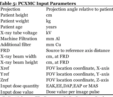
Table 5: PCXMC Input Parameters
PCXMC uses a computational phantom with anatomical data based on the mathematical hermaphrodite phantoms of Cristy and Eckerman.193-195 These phantoms describe patients of various ages: a new-born, 1 year-old, 5 year-old, 10 year-old, 15 year-old, and adult. The tissues simulated in PCXMC are soft tissue (1.04 g/cm3), lung tissue (0.296 g/cm3), and skeleton (1.40 g/cm3, newborn 1.22 g/cm3).193 Some changes have been made to the phantoms and internal organs to coincide with ICRP 103 tissue weighting factors.193 Examples of these changes include additions of the mouth mucosa, salivary gland, extrathoracic airways, and prostate, modelled with guidance from ICRP Publication 89 as well as other studies.193 In addition, the program allows phantom size to be adjusted to match patients of any weight or height. FOV can be freely adjusted relative to the patient.193
The program uses an Excel (Microsoft, Redmond, WA) spreadsheet for calculation of the total volume effective dose. Each line within the spreadsheet represents a single pulse of the scan. This means that a scan with 360 total pulses would have 360 lines in the spreadsheet. Within each line, the parameters of the machine and scan are entered. Projection represents the
Projection Projection angle relative to patient Patient height cm
Patient weight kg
Patient age years
X-ray tube voltage kV Machine Filtration mm Al Additional filter mm Cu
FRD Source to reference axis distance X-ray beam width cm, at FRD
X-ray beam height cm, at FRD
Xref FOV location coordinate, X-axis
Y ref FOV location coordinate, Y -axis
Zref FOV location coordinate, Z-axis
Input dose quantity EAK,EE,DAP,EAP or MAS Input dose value Dose value per image pulse
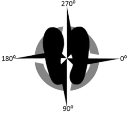
numerical angle of that individual pulse. The software angle orientation relative to the patient is represented in figure 1.
Figure 1: PCXMC angle orientation relative to patient
(As if looking up through the floor, so patient left is 0 degrees)
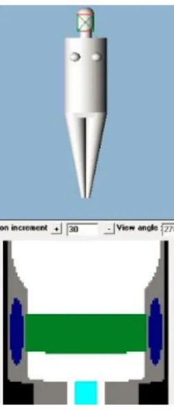
Considering the pathway of the source around the patient’s head, the starting angle of the first pulse and the ending angle of the last pulse were entered on the first and last lines respectively, with all the remaining intermediate pulse angles entered on the remaining lines.
The number of scan pulses and all pulse angles were obtained from the manufacturers, either from the machine documentation themselves, or through direct inquiry. Patient height, weight, and age similar to the phantom used in the correlating physical scan were entered. PCXMC settings for an adult 30 year-old are 178.6 cm height and 73.2 kg weight, and the child setting for a 10 year old is 139.8 cm height and 32.4 kg weight. This is similar in external
product documentation or directly from the manufacturer. The width and height of the x-ray beam field at the reference axis are calculated from the x-ray beam field at the receptor using trigonometry. Given the dimensions of the field at the receptor, the x-ray beam may be considered a square pyramid, with the source as the apex. The height of the pyramid is the source to receptor distance, obtained either from machine documentation or directly from the manufacturer. As the dimensions of the base and height of the pyramid are known, the field of view at the reference axis can be calculated.
The x-ray tube voltage was entered from the parameters of the specific scan. The x, y, and z references are the coordinates of the center of the rectangular scan field at the reference axis. PCXMC has a simulated scout window, shown in figure 2, which allows visual placement of the scan relative to the patient. Each simulated scan is situated to replicate phantom scan placement. The input dose quantity chosen for this research was mAs and dose area product (DAP). Each machine provides both mAs and DAP for each scan protocol. For each scan, these are divided by the number of scan pulses for that scan, and entered under the category “input dose value,” with the mAs per pulse on each line of the mAs scan, and the DAP per pulse on each line of the DAP scan. For each phantom scan protocol, one simulated scan was run using the mAs input value, and then another simulated scan using the DAP input value.
For the purpose of the mathematical evaluation, the program considers that the x-ray photons are emitted from a point source and then interact within the parameters specified in the scan (x-ray FOV size, patient reference axis, pulse angle, etc.). Pseudo-random numbers are generated to simulate photon direction, interaction distance, type of interacting atom,
interaction type with that atom, scatter angle, and energy loss. These photons are then followed in their interactions in the phantom using the probability of types of scatter or photoelectric absorption.193 The process of interactions is compiled to create a “photon history.” Many independent photon histories are created, which then are used to estimate the energy deposited in the simulated organs of the phantom.193
From this information, the program calculates the effective dose using both ICRP 103 and 60 values. The sum of each line effective dose is taken, representing the effective dose of the entire scan. For this study, only ICRP 103 values were evaluated. PCXMC 2.0 was run on a laptop computer (Lenovo, Morrisville, NC and Beijing, China) using Windows 7 (Microsoft, Redmond, WA).
Dosimetry values were calculated using these parameters and compared with phantom dosimetry results. The null hypothesis, that there is no statistically significant difference
between the dosimetry values of the anthropomorphic phantom and the calculated values of the PCXMC software, was tested.
RESULTS
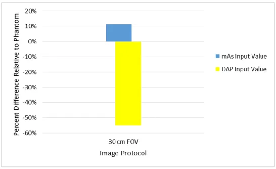
The percent difference of the PCXMC estimated doses relative to the phantom doses are given in figure 3-figure 6.
Figure 4: Sirona Galileos Comfort Plus PCXMC effective dose estimates relative to phantom
Figure 5: CS9300 PCXMC effective dose estimates relative to phantom
Figure 6: iCat FLX PCXMC effective dose estimates relative to phantom
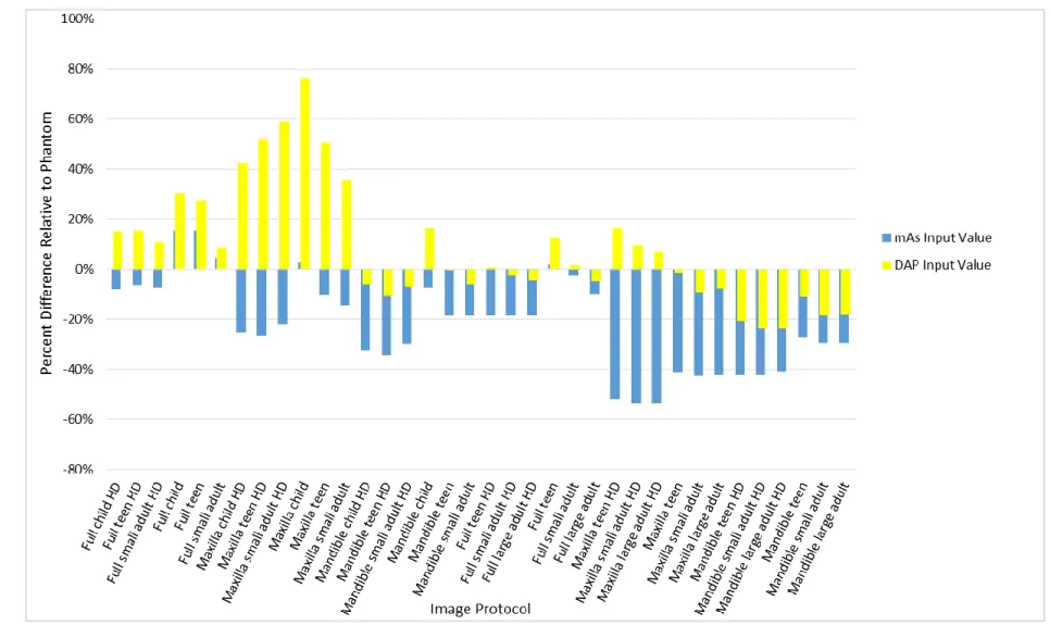
Using mAs as the input variable resulted in simulated effective doses at or below the ±20% target threshold 48% of the time. Increasing the threshold to ±30% would result in 60% success, and to ±50%, 77% success. Using DAP as the input variable resulted in simulated effective doses at or below the ±20% threshold 57% of the time. Increasing that threshold to ±30% would result in 70% success, and to ±50%, 82% success. Differences were as much as 300% on the CS9300 for certain small FOVs. Even though there are visual percent differences between using mAs or DAP, the chi-square analysis showed there was not a significant
association between input variable (mAs or DAP) and whether or not PCXMC predicted dose was within ±20% of the phantom measured effective dose χ2 (1)=1.791, p=.114.
The logistic regression results showed that the only consistently significant finding was FOV location. Those protocols strictly in the maxilla and above were less likely to stay below the target threshold, and those that encompassed both maxilla and mandible were more likely to stay below the target threshold. When mAs was used as the input variable, effective doses in larger volumes were slightly less likely to be below the target threshold. When DAP was used as the input variable, effective doses in the adult phantom were more likely to be below the target threshold. The results are shown in figure 7 and Figure 8.
Figure 7: Logistic Regression with mAs as the input variable. Variables examined included machine used, phantom used (adult or child), FOV location, FOV volume size, and phantom measured dose
Parameter DF Estimate SE
Wald Chi-Square
Pr > ChiSq
Machine CS9300 1 -0.1475 0.3429 0.1851 0.667
Machine iCat FLX 1 0.3782 0.4128 0.8396 0.3595
Phantom Used Adult 1 -0.5252 0.4698 1.2496 0.2636
Dose 1 -0.00338 0.00493 0.4701 0.493
FOV Location Full 1 2.0433 0.4315 22.4212 <.0001
FOV Location Maxilla 1 -1.5152 0.3899 15.1014 0.0001
FOV Volume (cm3) 1 -0.00089 0.00035 6.304 0.012
Figure 8: Logistic Regression with DAP as the input variable. Variables examined included machine used, phantom used (adult or child), FOV location, FOV volume size, and phantom measured dose.
The percentage of the software organ equivalent dose estimates that were within ±20% of the phantom measured doses are given in figure 9.
Figure 9: Percentage of PCXMC organ dose estimates within ±20% of phantom, with DAP or mAs as input variable.
Parameter DF Estimate SE
Wald Chi-Square
Pr > ChiSq
Machine CS9300 1 -0.6237 0.3343 3.4804 0.0621
Machine iCat FLX 1 -0.0098 0.3643 0.0007 0.9785
Phantom Used Adult 1 1.4437 0.4695 9.4547 0.0021
Dose 1 0.00597 0.00548 1.1836 0.2766
FOV Location Full 1 0.9107 0.3621 6.3241 0.0119
FOV Location Maxilla 1 -1.2947 0.3583 13.0584 0.0003
FOV Volume (cm3) 1 -0.00027 0.000222 1.4429 0.2297
In evaluating equivalent dose on the organs, the mucosa, salivary glands, and airway had the most estimates within the threshold using both mAs and DAP. Lymph nodes had none in both.
The chi-square analysis on the equivalent doses of all the organs shows that when using mAs as the input variable, there is a significant but only moderate association between the organ and whether the dose was within the phantom dose threshold (χ2 (9)=76.945, p<.001, Cramer’s V= .262). Using DAP as the input variable, the association was slightly stronger (χ2
(9)=168.714, p<.001, Cramer’s V= .388). Figure 10 and figure 11 show the standardized
residuals. Positive and negative values represents greater than or less than expected counts, and the number value represents the significance. All other organs were not significant. (See
Appendix 1 and 2)
Figure 10: Chi-square standardized residuals, with mAs as input value
Figure 11: Chi-square standardized residuals, with DAP as input value Organ Std. Residual
Salivary 4.2
Mucosa 3.6
Thyroid -3.2
Esophagus -3.9
Organ Std. Residual
Mucosa 7.3
Airway 4.6
Salivary 4.3
Skeleton -2.1
Brain -2.1
Esophagus -2.5
Thyroid -3.7
DISCUSSION
In evaluating of the significance of the FOV location, previous research has
demonstrated that when organs are partially within the x-ray field, doses can drastically differ between phantoms.197 While this doesn’t explain why mandibular FOVs were not significantly different, it does logically follow that as more organs are partially within the scan, the more variance between phantoms is encountered.
However, this does not explain the only significant finding relating to FOV size. When using mAs as the input variable, larger FOVs were slightly less likely of being within 20% of the phantom measured effective dose. Logically, it follows that a smaller FOV would have more organs partially within the scan, and accordingly, greater variability. Other than the fact that the likelihood ratio is so small (-0.00089) that it may be statistically, but not practically significant, this finding cannot be explained at this time.
The variance in adult versus child phantom when using DAP is consistent with previous research, that found significant changes in effective dose without any change in DAP.198
Additionally, studies have shown vast differences in conversion factors when attempting to equate DAP with effective dose.165, 199 In the protocols that scanned both adult and child
phantoms, DAP did not change between the two. Child phantom organ positioning may have an even greater effect on effective dose deviations in this instance, as more organs, particularly the thyroid, are included or proximal to the beam.192 Differences in organ position can have
Limitations
Initial concerns were regarding the machine specific FOV geometry, since PCXMC calculates the scan as a cylinder. Two of the machines evaluated, the NewTom 3G and Galileos, have spherical FOVs, while the CS9300 and iCat FLX have a cylindrical FOVs. However, no significant difference was found between the machines themselves.
Additionally, as PCXMC allows for FOV placement in all three planes (X, Y, and Z) the positioning scan, particularly with smaller protocols, will always be a potential source of error. While a scout window is present within PCXMC, positioning still requires human judgment. To test this, software scans were run with several cm differences in positioning. Estimated effective dose from the software varied less than 5% with different positions, unless the exam bordered the thyroid. Greater inclusion of the thyroid within the scan by moving the target inferiorly increased the estimated effective dose upwards of 15%, with dramatic increases in equivalent dose to the organ itself. However, the potential variation is still present, and is illustrated in several 5x5 FOV protocols in the CS9300, which demonstrated some of the highest variation in this study, with differences ranging from 3% to above 200 and 300% difference from the
phantom. PCXMC overestimated doses in 13 out of 14 instances. In this machine specific subset of imaging protocols, there was no consistency on location relative to percent difference
(posterior/anterior FOV, or maxillary/mandibular FOV)
Another significant potential source of error is the choice of the phantom itself. There are a few different types of computational phantoms. The phantom used in PCXMC is a
phantoms are “voxel” or “tomographic” phantoms. These phantoms use magnetic resonance (MR) or CT image information to construct organ and body structure.202 A third recent type of computational phantom has been developed – called “hybrid” or “boundary representation” (BREP) phantoms.184, 203 These phantoms have the benefit of being easily deformable – which allows the alteration to fit different organ shapes or different body types. These may be constructed with a polygonal mesh – a set of faces that determine the polyhedral shape of organs and other structures. These newer phantoms allow for simulation of particularly complex anatomies.184
The computational phantoms with more realistic anatomy have been compared to the initial stylized phantoms.197, 203-207 Exposure levels in organs between certain phantoms (and classes of phantoms) can vary significantly, and relate to organ shape and distribution.202, 207 Effective dose can depend strongly on the choice of phantom, organ positions, and field size and position.200 The phantom used in PCXMC includes soft tissue, lung tissue, and skeleton. The ATOM phantom includes soft tissue, spinal cord, spinal disks, lung, brain, and sinus, and the RANDO phantom includes soft tissue, lungs, and natural human skeletons.176, 177 Although phantom tissue attenuation factors aim to follow ICRP recommendations, there are natural variations between human bone and polymers, as well as inherent differences between
systems.177, 193 Even when comparing different phantoms of the same type (e.g. voxel phantoms with voxel phantoms), differences in effective dose have been found to range up to nearly
50%.206 Of note is when there is inability to alter the orientation of the phantom head within the scan to more appropriately model patient head positioning. Since positioning within the scan has been shown to make a significant difference on organ and effective dose,94, 96, 99, 198 this results in the fact that phantoms intended for general dosimetry may ultimately be limited and present with inherent variance when used in dental CBCT application.
PCXMC Previous Validation Studies
Studies comparing PCXMC with other Monte Carlo programs and phantoms have shown varying levels of agreement.139, 197 In evaluating PCXMC with MCNP, a Monte Carlo program from the Los Alamos National Laboratory (LANL) Schultz and co-workers found that while the PCXMC estimated individual organ doses during pediatric cardiology procedures sometimes varied considerably from the MCNP values, effective dose had more reasonable agreement.139 Since the effective doses evaluated were in mSv, the acceptable margin of error included differences of up to nearly 800 µSv.139
In comparing PCXMC with a voxel phantom and MCNPX (LANL, Los Alamos, NM), Smans and co-workers found increased differences in mean organ dose between phantoms when organs were partially within the x-ray field, as much as 700%.197 Even when the different phantoms underwent total body irradiation, differences in mean organ doses between the phantoms ranged from 1%-96%.197
Another study by Helmrot and co-workers found that software estimated absorbed doses agreed within ±50% of measured absorbed doses to the uterus.208 The difference between PCXMC estimates and measured absorbed dose in this study was commonly within the range of 0.1-0.2 mGy (100-200 µGy) and varied as much as 5mGy.208 Wood and co-workers evaluated the CBCT dose associated with a Varian on-board-imager CBCT (OBI, Varian Medical Systems, Palo Alto, CA) against RANDO phantom TLDs. The authors found that the majority of software estimated organ doses were within 20%.146 As the doses were in mGy, the smallest number difference was 0.3 mGy, or 300 µGy. Overall, even though PCXMC was shown to have
reasonable agreement with the comparison phantoms, Monte Carlo programs, and other dose measurements, the acceptable difference margin in those studies often exceeded the largest doses evaluated within this present study.
Organ doses
dosimetry accounts for lymph nodes by averaging from dosimeters near anatomical head and neck lymph node locations. Additionally, precision of the dose estimate may be low if the dose to the organ is low.193 Common doses in dental CBCT are 10-1000 times less than those
protocols used in studies cited previously. This primarily explains the low global success rate in organ dose estimation. This reiterates an important issue – since effective dose is compiled from organ doses, differences between phantoms can lead to significant variations in dose.
Figure 12: PCXMC lymph node dose calculation
Dental CBCT Dose concerns: Are they worth discussing?
a population of patients results in a public health concern that cannot be deemed insignificant.165 Thus, dental CBCT doses ARE worth discussing.
Future Directions
CONCLUSIONS
APPENDIX 1: MAS INPUT VARIABLE ORGAN CHI-SQUARE ANALYSIS
Organs Coded * mAs Hit Threshold? Crosstabulation
mAs Hit Threshold?
Total
NO YES
Organs Coded Marrow Count 89 23 112
Expected
Count 89.8 22.2 112.0
% within
Organs Coded 79.5% 20.5% 100.0%
% within mAs
Hit Threshold? 9.9% 10.4% 10.0%
% of Total 7.9% 2.1% 10.0%
Std. Residual -.1 .2
Thyroid Count 105 7 112
Expected
Count 89.8 22.2 112.0
% within
Organs Coded 93.8% 6.3% 100.0%
% within mAs
Hit Threshold? 11.7% 3.2% 10.0%
% of Total 9.4% .6% 10.0%
Std. Residual 1.6 -3.2
Esophagus Count 108 4 112
Expected
Count 89.8 22.2 112.0
% within
Organs Coded 96.4% 3.6% 100.0%
% within mAs
Hit Threshold? 12.0% 1.8% 10.0%
% of Total 9.6% .4% 10.0%
Std. Residual 1.9 -3.9
Skin Count 94 18 112
Expected
Count 89.8 22.2 112.0
% within
Organs Coded 83.9% 16.1% 100.0%
% within mAs
Hit Threshold? 10.5% 8.1% 10.0%
% of Total 8.4% 1.6% 10.0%
Std. Residual .4 -.9
Skeleton Count 91 21 112
Expected
Count 89.8 22.2 112.0
% within
Organs Coded 81.3% 18.8% 100.0%
% within mAs
% of Total 8.1% 1.9% 10.0%
Std. Residual .1 -.3
Salivary Count 70 42 112
Expected
Count 89.8 22.2 112.0
% within
Organs Coded 62.5% 37.5% 100.0%
% within mAs
Hit Threshold? 7.8% 18.9% 10.0%
% of Total 6.3% 3.8% 10.0%
Std. Residual -2.1 4.2
Brain Count 97 15 112
Expected
Count 89.8 22.2 112.0
% within
Organs Coded 86.6% 13.4% 100.0%
% within mAs
Hit Threshold? 10.8% 6.8% 10.0%
% of Total 8.7% 1.3% 10.0%
Std. Residual .8 -1.5
Airway Count 82 30 112
Expected
Count 89.8 22.2 112.0
% within
Organs Coded 73.2% 26.8% 100.0%
% within mAs
Hit Threshold? 9.1% 13.5% 10.0%
% of Total 7.3% 2.7% 10.0%
Std. Residual -.8 1.7
Muscle Count 89 23 112
Expected
Count 89.8 22.2 112.0
% within
Organs Coded 79.5% 20.5% 100.0%
% within mAs
Hit Threshold? 9.9% 10.4% 10.0%
% of Total 7.9% 2.1% 10.0%
Std. Residual -.1 .2
Mucosa Count 73 39 112
Expected
Count 89.8 22.2 112.0
% within
Organs Coded 65.2% 34.8% 100.0%
% within mAs
Hit Threshold? 8.1% 17.6% 10.0%
% of Total 6.5% 3.5% 10.0%
Std. Residual -1.8 3.6
Expected
Count 898.0 222.0 1120.0
% within
Organs Coded 80.2% 19.8% 100.0%
% within mAs
Hit Threshold? 100.0% 100.0% 100.0%
% of Total 80.2% 19.8% 100.0%
Chi-Square Tests
Value df
Asymp. Sig. (2-sided) Exact Sig. (2-sided) Exact Sig. (1-sided) Point Probability Pearson
Chi-Square 76.945
a 9 .000 .000
Likelihood
Ratio 82.788 9 .000 .
b
Fisher's Exact
Test .
b .b
Linear-by-Linear Association
26.943c 1 .000 .000 .000 .000
N of Valid
Cases 1120
a. 0 cells (0.0%) have expected count less than 5. The minimum expected count is 22.20.
b. Cannot be computed because there is insufficient memory.
c. The standardized statistic is 5.191.
Directional Measures Value Asymp. Std. Errora Approx. Tb Approx. Sig. Exact Sig. Nominal by Nominal
Lambda Symmetric .031 .013 2.353 .019
Organs Coded
Dependent .038 .016 2.353 .019
mAs Hit Threshold? Dependent
0.000 0.000 .c .c
Goodman and Kruskal tau
Organs Coded
Dependent .008 .002 .000d .000
mAs Hit Threshold? Dependent
.069 .014 .000d .e
a. Not assuming the null hypothesis.
b. Using the asymptotic standard error assuming the null hypothesis.
c. Cannot be computed because the asymptotic standard error equals zero.
d. Based on chi-square approximation
Symmetric Measures
Value
Approx.
Sig. Exact Sig.
Nominal by Nominal
Phi .262 .000 .000
Cramer's V .262 .000 .000
Contingency
Coefficient .254 .000 .000
APPENDIX 2: DAP INPUT VARIABLE ORGAN CHI-SQUARE ANALYSIS
Organs Coded * DAP Hit Threshold? Crosstabulation
DAP Hit Threshold?
Total
NO YES
Organs Coded Marrow Count 96 16 112
Expected
Count 92.9 19.1 112.0
% within
Organs Coded 85.7% 14.3% 100.0%
% within DAP
Hit Threshold? 10.3% 8.4% 10.0%
% of Total 8.6% 1.4% 10.0%
Std. Residual .3 -.7
Thyroid Count 109 3 112
Expected
Count 92.9 19.1 112.0
% within
Organs Coded 97.3% 2.7% 100.0%
% within DAP
Hit Threshold? 11.7% 1.6% 10.0%
% of Total 9.7% .3% 10.0%
Std. Residual 1.7 -3.7
Esophagus Count 104 8 112
Expected
Count 92.9 19.1 112.0
% within
Organs Coded 92.9% 7.1% 100.0%
% within DAP
Hit Threshold? 11.2% 4.2% 10.0%
% of Total 9.3% .7% 10.0%
Std. Residual 1.2 -2.5
Skin Count 111 1 112
Expected
Count 92.9 19.1 112.0
% within
Organs Coded 99.1% .9% 100.0%
% within DAP
Hit Threshold? 11.9% .5% 10.0%
% of Total 9.9% .1% 10.0%
Std. Residual 1.9 -4.1
Skeleton Count 102 10 112
Expected
Count 92.9 19.1 112.0
% within
Organs Coded 91.1% 8.9% 100.0%
% within DAP
% of Total 9.1% .9% 10.0%
Std. Residual .9 -2.1
Salivary Count 74 38 112
Expected
Count 92.9 19.1 112.0
% within
Organs Coded 66.1% 33.9% 100.0%
% within DAP
Hit Threshold? 8.0% 19.9% 10.0%
% of Total 6.6% 3.4% 10.0%
Std. Residual -2.0 4.3
Brain Count 102 10 112
Expected
Count 92.9 19.1 112.0
% within
Organs Coded 91.1% 8.9% 100.0%
% within DAP
Hit Threshold? 11.0% 5.2% 10.0%
% of Total 9.1% .9% 10.0%
Std. Residual .9 -2.1
Airway Count 73 39 112
Expected
Count 92.9 19.1 112.0
% within
Organs Coded 65.2% 34.8% 100.0%
% within DAP
Hit Threshold? 7.9% 20.4% 10.0%
% of Total 6.5% 3.5% 10.0%
Std. Residual -2.1 4.6
Muscle Count 97 15 112
Expected
Count 92.9 19.1 112.0
% within
Organs Coded 86.6% 13.4% 100.0%
% within DAP
Hit Threshold? 10.4% 7.9% 10.0%
% of Total 8.7% 1.3% 10.0%
Std. Residual .4 -.9
Mucosa Count 61 51 112
Expected
Count 92.9 19.1 112.0
% within
Organs Coded 54.5% 45.5% 100.0%
% within DAP
Hit Threshold? 6.6% 26.7% 10.0%
% of Total 5.4% 4.6% 10.0%
Std. Residual -3.3 7.3
Expected
Count 929.0 191.0 1120.0
% within
Organs Coded 82.9% 17.1% 100.0%
% within DAP
Hit Threshold? 100.0% 100.0% 100.0%
% of Total 82.9% 17.1% 100.0%
Chi-Square Tests
Value df
Asymp. Sig. (2-sided) Exact Sig. (2-sided) Exact Sig. (1-sided) Point Probability Pearson
Chi-Square 168.714
a 9 .000 .000
Likelihood
Ratio 168.875 9 .000 .
b
Fisher's Exact
Test .
b .b
Linear-by-Linear Association
70.876c 1 .000 .000 .000 .000
N of Valid
Cases 1120
a. 0 cells (0.0%) have expected count less than 5. The minimum expected count is 19.10.
b. Cannot be computed because there is insufficient memory.
c. The standardized statistic is 8.419.
Directional Measures Value Asymp. Std. Errora Approx. Tb Approx. Sig. Exact Sig. Nominal by Nominal
Lambda Symmetric .042 .013 3.033 .002
Organs Coded
Dependent .050 .016 3.033 .002
DAP Hit Threshold? Dependent
0.000 0.000 .c .c
Goodman and Kruskal tau
Organs Coded
Dependent .017 .002 .000d .000
DAP Hit Threshold? Dependent
.151 .022 .000d .e
a. Not assuming the null hypothesis.
b. Using the asymptotic standard error assuming the null hypothesis.
c. Cannot be computed because the asymptotic standard error equals zero.
d. Based on chi-square approximation
Symmetric Measures
Value
Approx.
Sig. Exact Sig.
Nominal by Nominal
Phi .388 .000 .000
Cramer's V .388 .000 .000
Contingency
Coefficient .362 .000 .000
REFERENCES
1. Eckhardt R. Stan Ulam, John von Neumann, and the Monte Carlo method. Los Alamos Science 1987;15:131-37.
2. Ulam SM. Adventures of a mathematician. New York: Scribner; 1976.
3. Everett CJ, Ulam S. Multiplicative Systems: I. Proc Natl Acad Sci U S A 1948;34(8):403-5.
4. Metropolis N. The Beginning of the Monte Carlo Method. Los Alamos Science 1987;15:125-30.
5. Richtmyer Rv, J. Statistical Methods in Neutron Diffusion. Los Alamos: Los Alamos National Laboratory; 1947.
6. Metropolis N, Ulam S. The Monte Carlo method. J Am Stat Assoc 1949;44(247):335-41.
7. Kalos MW, PA. Monte Carlo Methods, 2nd Edition. 2nd Edition ed. Darmstadt, Federal Republic of Germany: Wiley-Blackwell; 2008.
8. Lux I, Koblinger L. Monte Carlo particle transport methods: neutron and photon calculations. Boca Raton: CRC Press; 1991.
9. Norris J. Markov Chains. Cambridge, United Kingdom: Cambridge University Press; 1998.
10. Draper NR. The Cambridge Dictionary of Statistics, Fourth Edition by B. S. Everitt, A. Skrondal. International Statistical Review 2011;79(2):273-74.
11. PubMed search "monte carlo".
"http://www.ncbi.nlm.nih.gov/pubmed/?term=%22monte+carlo%22". 2015.
12. Rogers DW. Fifty years of Monte Carlo simulations for medical physics. Phys Med Biol 2006;51(13):R287-301.
14. Abuhaimed A, C JM, Sankaralingam M, D JG, McJury M. An assessment of the efficiency of methods for measurement of the computed tomography dose index (CTDI) for cone beam (CBCT) dosimetry by Monte Carlo simulation. Phys Med Biol 2014;59(21):6307-26.
15. Alaei P, Spezi E. Commissioning kilovoltage cone-beam CT beams in a radiation therapy treatment planning system. J Appl Clin Med Phys 2012;13(6):3971.
16. Teymurazyan A, Rowlands JA, Pang G. Monte Carlo simulation of a quantum noise limited Cerenkov detector based on air-spaced light guiding taper for megavoltage x-ray imaging. Med Phys 2014;41(4):041907.
17. Son K, Cho S, Kim JS, and co-workers. Evaluation of radiation dose to organs during kilovoltage cone-beam computed tomography using Monte Carlo simulation. J Appl Clin Med Phys 2014;15(2):4556.
18. Poirier Y, Kouznetsov A, Koger B, Tambasco M. Experimental validation of a kilovoltage x-ray source model for computing imaging dose. Med Phys 2014;41(4):041915.
19. McMillan K, McNitt-Gray M, Ruan D. Development and validation of a measurement-based source model for kilovoltage cone-beam CT Monte Carlo dosimetry simulations. Med Phys 2013;40(11):111907.
20. Fleckenstein J, Jahnke L, Lohr F, Wenz F, Hesser J. Development of a Geant4 based Monte Carlo Algorithm to evaluate the MONACO VMAT treatment accuracy. Z Med Phys 2013;23(1):33-45.
21. Ding GX, Munro P. Radiation exposure to patients from image guidance procedures and techniques to reduce the imaging dose. Radiother Oncol 2013;108(1):91-8.
22. Roberts DA, Hansen VN, Thompson MG, and co-workers. Kilovoltage energy imaging with a radiotherapy linac with a continuously variable energy range. Med Phys
2012;39(3):1218-26.
23. Qiu Y, Moiseenko V, Aquino-Parsons C, Duzenli C. Equivalent doses for gynecological patients undergoing IMRT or RapidArc with kilovoltage cone beam CT. Radiother Oncol 2012;104(2):257-62.
25. Kim S, Song H, Samei E, Yin FF, Yoshizumi TT. Computed tomography dose index and dose length product for cone-beam CT: Monte Carlo simulations. J Appl Clin Med Phys 2011;12(2):3395.
26. Kim S, Yoshizumi T, Toncheva G, and co-workers. Estimation of computed tomography dose index in cone beam computed tomography: MOSFET measurements and Monte Carlo simulations. Health Phys 2010;98(5):683-91.
27. Kim S, Yoshizumi TT, Toncheva G, Frush DP, Yin FF. Estimation of absorbed doses from paediatric cone-beam CT scans: MOSFET measurements and Monte Carlo simulations. Radiat Prot Dosimetry 2010;138(3):257-63.
28. Kim S, Yoo S, Yin FF, Samei E, Yoshizumi T. Kilovoltage cone-beam CT: comparative dose and image quality evaluations in partial and full-angle scan protocols. Med Phys 2010;37(7):3648-59.
29. Dobler B, Streck N, Klein E, and co-workers. Hybrid plan verification for intensity-modulated radiation therapy (IMRT) using the 2D ionization chamber array I'mRT MatriXX--a feasibility study. Phys Med Biol 2010;55(2):N39-55.
30. Ding A, Gu J, Trofimov AV, Xu XG. Monte Carlo calculation of imaging doses from diagnostic multidetector CT and kilovoltage cone-beam CT as part of prostate cancer treatment plans. Med Phys 2010;37(12):6199-204.
31. Wulff J, Ubrich F, Zink K. Comment on "Monte Carlo simulation of an x-ray volume imaging cone beam CT unit" [Med. Phys. 36, 127-136 (2009)]. Med Phys
2009;36(3):1039; author reply 40.
32. Spezi E, Downes P, Radu E, Jarvis R. Monte Carlo simulation of an x-ray volume imaging cone beam CT unit. Med Phys 2009;36(1):127-36.
33. Downes P, Jarvis R, Radu E, Kawrakow I, Spezi E. Monte Carlo simulation and patient dosimetry for a kilovoltage cone-beam CT unit. Med Phys 2009;36(9):4156-67.
34. Chow JC, Leung MK, Van Dyk J. Variations of lung density and geometry on
inhomogeneity correction algorithms: a Monte Carlo dosimetric evaluation. Med Phys 2009;36(8):3619-30.
36. Gu J, Bednarz B, Xu XG, Jiang SB. Assessment of patient organ doses and effective doses using the VIP-Man adult male phantom for selected cone-beam CT imaging procedures during image guided radiation therapy. Radiat Prot Dosimetry 2008;131(4):431-43.
37. Ding GX, Duggan DM, Coffey CW. Accurate patient dosimetry of kilovoltage cone-beam CT in radiation therapy. Med Phys 2008;35(3):1135-44.
38. Chow JC, Leung MK, Islam MK, Norrlinger BD, Jaffray DA. Evaluation of the effect of patient dose from cone beam computed tomography on prostate IMRT using Monte Carlo simulation. Med Phys 2008;35(1):52-60.
39. Ding GX, Duggan DM, Coffey CW. Characteristics of kilovoltage x-ray beams used for cone-beam computed tomography in radiation therapy. Phys Med Biol 2007;52(6):1595-615.
40. Vanderstraeten B, Reynaert N, Paelinck L, and co-workers. Accuracy of patient dose calculation for lung IMRT: A comparison of Monte Carlo, convolution/superposition, and pencil beam computations. Med Phys 2006;33(9):3149-58.
41. Reynaert N, Coghe M, De Smedt B, and co-workers. The importance of accurate linear accelerator head modelling for IMRT Monte Carlo calculations. Phys Med Biol
2005;50(5):831-46.
42. Spezi E, Lewis DG, Smith CW. Monte Carlo simulation and dosimetric verification of radiotherapy beam modifiers. Phys Med Biol 2001;46(11):3007-29.
43. Francescon P, Cavedon C, Reccanello S, Cora S. Photon dose calculation of a three-dimensional treatment planning system compared to the Monte Carlo code BEAM. Med Phys 2000;27(7):1579-87.
44. Chytyk-Praznik K, VanUytven E, vanBeek TA, Greer PB, McCurdy BM. Model-based prediction of portal dose images during patient treatment. Med Phys 2013;40(3):031713.
45. Teymurazyan A, Pang G. Monte Carlo simulation of a novel water-equivalent electronic portal imaging device using plastic scintillating fibers. Med Phys 2012;39(3):1518-29.
46. van Elmpt W, Petit S, De Ruysscher D, Lambin P, Dekker A. 3D dose delivery verification using repeated cone-beam imaging and EPID dosimetry for stereotactic body