PubMedCentral-PMC5065050.pdf

Automated quanti

fi

cation of cerebral edema following hemispheric

infarction: Application of a machine-learning algorithm to evaluate CSF

shifts on serial head CTs

Yasheng Chen

, Rajat Dhar

, Laura Heitsch

, Andria Ford

, Israel Fernandez-Cadenas

, Caty Carrera

,

Joan Montaner

, Weili Lin

, Dinggang Shen

, Hongyu An

, Jin-Moo Lee

⁎

a

Department of Neurology, Washington University, St. Louis, MO 63110, USA

b

Emergency Medicine, Washington University, St. Louis, MO 63110, USA

c

Stroke Pharmacogenomics and Genetics, Fundacio Docencia i Recerca MutuaTerrassa, Mutua de Terrassa Hospital, Terrassa, Barcelona, Spain

d_{Neurovascular Research Laboratory, Vall d'Hebron Institute of Research, Universitat Autonoma de Barcelona, Barcelona, Spain} e

Biomedical Research Imaging Center, University of North Carolina, Chapel Hill, NC 27599, USA

f

Dept. of Radiology, University of North Carolina, Chapel Hill, NC 27599, USA

g

Department of Brain and Cognitive Engineering, Korea University, Seoul 02841, Republic of Korea

h

Radiology, Washington University, St. Louis, MO 63110, USA

i

Biomedical Engineering, Washington University, St. Louis, MO 63110, USA

a b s t r a c t

a r t i c l e i n f o

Article history:

Received 24 June 2016

Received in revised form 22 September 2016 Accepted 24 September 2016

Available online 26 September 2016

Although cerebral edema is a major cause of death and deterioration following hemispheric stroke, there remains no validated biomarker that captures the full spectrum of this critical complication. We recently demonstrated that reduction in intracranial cerebrospinalfluid (CSF) volume (ΔCSF) on serial computed tomography (CT) scans provides an accurate measure of cerebral edema severity, which may aid in early triaging of stroke patients for craniectomy. However, application of such a volumetric approach would be too cumbersome to perform man-ually on serial scans in a real-world setting. We developed and validated an automated technique for CSF seg-mentation via integration of random forest (RF) based machine learning with geodesic active contour (GAC) segmentation. The proposed RF + GAC approach was compared to conventional Hounsfield Unit (HU) thresholding and RF segmentation methods using Dice similarity coefficient (DSC) and the correlation of volu-metric measurements, with manual delineation serving as the ground truth. CSF spaces were outlined on scans performed at baseline (b6 h after stroke onset) and early follow-up (FU) (closest to 24 h) in 38 acute ischemic stroke patients. RF performed significantly better than optimized HU thresholding (pb10−4in baseline and pb10−5in FU) and RF + GAC performed significantly better than RF (pb10−3in baseline and pb10−5in FU). Pearson correlation coefficients between the automatically detectedΔCSF and the ground truth werer= 0.178 (p = 0.285),r= 0.876 (pb10−6) andr= 0.879 (pb10−6) for thresholding, RF and RF + GAC, respective-ly, with a slope closer to the line of identity in RF + GAC. When we applied the algorithm trained from images of one stroke center to segment CTs from another center, similarfindings held. In conclusion, we have developed and validated an accurate automated approach to segment CSF and calculate its shifts on serial CT scans. This al-gorithm will allow us to efficiently and accurately measure the evolution of cerebral edema in future studies in-cluding large multi-site patient populations.

© 2016 The Authors. Published by Elsevier Inc. This is an open access article under the CC BY-NC-ND license (http://creativecommons.org/licenses/by-nc-nd/4.0/).

Keywords:

Active contour Cerebral edema CSF segmentation Ischemic stroke CT Mass effect Random forest

1. Introduction

Cerebral edema, the pathologic accumulation of excess water inside brain tissue, is a major cause of death and deterioration following ische-mic stroke and other brain injuries (Krieger et al., 1999; Rosenberg,

1999, 2000). Under the Monro-Kellie doctrine, compensation for this swelling must occur given the rigid confines of the cranium, with paral-lel reductions in the volume of other intracranial compartments such as blood and cerebrospinalfluid (CSF). If cerebral edema progresses be-yond the point where compensation has been exhausted, then intracra-nial compartmental pressure will rise, leading to brain herniation (Hacke et al., 1996). By opening the cranial vault (hence bypassing the restrictions of the Monro-Kellie doctrine), decompressive hemicraniectomy (DHC) is effective in preventing herniation and ⁎ Corresponding author at: Department of Neurology, Washington University School of

Medicine, 660 S. Euclid Ave, Campus Box 8111, St. Louis, MO 63110, USA.

E-mail address:[email protected](J.-M. Lee).

http://dx.doi.org/10.1016/j.nicl.2016.09.018

2213-1582/© 2016 The Authors. Published by Elsevier Inc. This is an open access article under the CC BY-NC-ND license (http://creativecommons.org/licenses/by-nc-nd/4.0/). Contents lists available atScienceDirect

NeuroImage: Clinical

death in patients with malignant cerebral edema after large hemispher-ic infarction (LHI) (Vahedi et al., 2007). This benefit requires early selec-tion of patients with malignant edema for DHC, ideally prior to development of herniation and within 48 h. Current approaches to sur-gical triage require high stroke severity coupled with large infarct seen either on delayed CT images or acute MRI (Thomalla et al., 2010). How-ever, neither NIHSS nor infarct volume is a direct measure of cerebral edema, leading to misclassification of patients for an invasive neurosur-gical procedure or delayed diagnosis until herniation occurs.

We have recently proposed that measuring reduction in CSF volume can provide a more direct and sensitive biomarker of edema. This can be accurately measured after volumetric segmentation of CSF from serial CT scans acquired at baseline and follow-up (FU) in patients with hemi-spheric infarction (Dhar et al., 2016). This CT-based approach may allow early and accurate identification of those at risk for developing malig-nant cerebral edema. However, manual segmentation of hemispheric CSF on two or more CT scans is time-consuming and impractical to apply to widespread rapid stroke triage decision-making. It is also im-possible for manual delineation to analyze the large datasets from multi-center stroke cohorts required to study the kinetics, predictive factors and genetic underpinnings of cerebral edema formation. Simple threshold-based approaches (as have been used to segment CSF on baseline stroke scans) may not accurately delineate CSF on FU CT scans where hypodense evolving infarct is hard to distinguish from sur-rounding CSF (Minnerup et al., 2011). The objective of this study was to develop an automated advanced CSF segmentation approach that is able to accurately quantify CSF volumetric changes from serial CT scans in the acute phase of ischemic stroke.

2. Materials and methods

2.1. Patients

We retrospectively identified patients with hemispheric infarction and cerebral edema of varying degrees from a stroke cohort enrolled in a prospective stroke study at two institutions. Eligibility criteria in-cluded: 1) baseline NIHSS≥8; 2) baseline head CT obtained within 6 h of stroke onset; 3) FU CT obtained at 6–48 h after stroke onset; 4) FU CT confirming hemispheric infarction and some degree of edema (i.e., sulcal and/or ventricular effacement with or without midline shift, MLS); 5) no parenchymal hematoma on FU CT. If more than one FU CT was performed, the scan closest to 24-hours was selected for analysis, as long as it was performed prior to any decompressive surgery. We have included 38 patients with hemispheric infarction, with 26 patients from Washington University/Barnes-Jewish Hospital, St. Louis, MO (center A) and 12 patients from Vall d'Hebron Hospital, Barcelona, Spain (center B). All subjects (or their proxy) provided informed con-sent and the study was approved by institutional review boards at

each center. Demographic and clinical characteristics of the study pop-ulation are given inTable 1.

2.2. Manual delineation

CSF was outlined using the MIPAV (Medical Image Processing, Anal-ysis, and Visualization) software package, as has been previously de-scribed (Dhar et al., 2016). CSF volume was segregated into compartments including hemispheric sulci and lateral ventricles, both ipsilateral (IL) and contralateral (CL) to the side of infarction. The third ventricle and the perimesencephalic and suprasellar cisterns were also outlined and included in total CSF volume. Total hemispheric CSF volume was quanti_fied on each CT scan as the sum of all CSF spaces and change in volume (ΔCSF) was calculated as the reduction in volume between these two scans (i.e., FU vs. baseline volume). Two raters sep-arately segmented CSF on a subset of scans and inter-rater reliability for manual volumetric segmentation of CSF was found to be 0.92. Manual CSF delineation was saved as image masks for comparison with auto-mated segmentation.

2.3. Pseudo-affine image registration

CT images consist of stacks of axial images with a thick slice separa-tion of 5 mm. In order to align CTs from different patients (with different orientation and head size) to a normalized frame to reduce geometrical variability, we adopted a pseudo af_fine registration to co-register all the CT images to a pre-chosen well-positioned template. In the affine trans-formation matrix, we restricted shears and rotations involving the foot to head direction, so that a 2D image slice remains a plane after transfor-mation. This warping process only allows 3D translation, in-plane rota-tion, scaling and shear. Following this registration step, the ground truth (i.e. manual) CSF segmentation masks were also transformed towards the template with the same transformation matrix. Besides making the sulci more consistently oriented, this warping process also allowed us to perform training of one random forest in this template frame for future deployment.

2.4. Random forest CSF classification

Our training-based CSF segmentation is a supervised learning pro-cess. Random forests (RF) (Breiman, 2001) has recently been applied to medical image segmentation with promising results (Geremia et al., 2011;Mitra et al., 2014). This hierarchical approach learns how to effi -ciently classify brain voxels by creating a large forest of multiple inde-pendent decision-trees derived from random subsets of the sample of CT scans provided (e.g. sets 1 through N, inFig. 1A). Initially, all samples in a subset (e.g. set 1 inFig. 1A) are pushed down from the root node of a tree to either the left or right branches (subsets S1 and S2) depending upon which route will achieve more ordered organization. Data is suc-cessively partitioned to optimize discrimination or until: 1) maximal tree depth is reached; 2) the minimal number of samples being divided is reached; or 3) all samples belong to the same class. RF then leverages this cluster of derived models to optimally segment each voxel (i.e. into CSF or other). To optimize classification, the Gini impurity index is re-duced through the splitting process. The calculation of this index is given in Eq.(1), withpkas the fraction of items labeled with valuek and the total cluster numberK. Gini impurity is a measure of how often an element is incorrectly labeled and it reaches zero when all the cases within a node all belong to a single class.

Gini¼∑K

k¼1pkð1−pkÞ ð1Þ

At each node split, the sum of Gini impurity from the two descen-dent nodes is less than the parent node. Finally, random forest takes ad-vantage of the concept of ensemble by training multiple trees with the repeated sampling of the training set. As a result, this supervised

Table 1

Demographic and clinical characteristics of the study population.

Variable/center Washington University, St. Louis

Vall d'Hebron, Barcelona

Number of subjects 26 12

Age, years 61 (52–80) 74 (56–82)

Gender, female 11 (42%) 5 (42%)

Race, white 18 (69%) 12 (100%)

Admission NIHSS 15 (10–19) 17 (11−21) Treated with tPA 21 (81%) 12 (100%) ASPECTS on baseline CT 9 (8–10) 9 (8–10) Time between baseline and FU,

hours

18 (13–34) 24 (18–27)

Midline shift, mla

0 (0–2.4) 0.5 (0–1.4)

Notes. Categorical variables are present as n (%); continuous variables are presented as medians (interquartile range).

a

Infarct volume and midline shift were assessed as visible on early FU CT scans.

Fig. 2.Demonstration of CSF segmentation results using Hounsfield Unit thresholding (A), RF (B) and RF + GAC (C) methods. Yellow regions represent the overlap between automated segmentation and ground truth (manual segmentation). Red and green regions represent under- and over-segmented CSF regions, respectively. (For interpretation of the references to color in thisfigure legend, the reader is referred to the web version of this article.)

learning method is able to cluster complex patterns within the sample while not over-fitting the data. An illustration of this machine learning method is given inFig. 1A.

Another advantage of RF classifier is that the prediction step is very efficient. The prediction of the class that one sample belongs to only in-volves pushing down the sample in each tree from the root node, and comparing one feature value with the stored threshold at the node to decide to travel either to the left or to the right descendant branch until a leaf node is reached. The calculation roughly takes the same amount of time as performing subtractions multiple times (depth of the tree∗number of trees).

In this study, we trained two random forest classifiers for baseline and FU scans, respectively. We utilized1-,2-and3-rectangle Haar-like features (features in a digital image used for object recognition) in our application computed through moving 1, 2 and 3 neighboring small squares (of size 5 × 5) in both horizontal and vertical directions one pixel at a time to span all the possible locations within a larger 11 × 11 window (Fig. 1B). The1-rectagle Haar-like features were com-puted as the average of the CT intensity inside the small square. The2 -rectangle Haar-like features were computed as the difference between

the averaged CT intensities from the two neighboring squares. The3 -rectangle Haar-like features were computed by subtracting the aver-aged CT intensity inside the center window from the summation of the average CT values inside the two outside squares. The training sam-ples were extracted from random locations from both CSF and non-CSF brain regions in a balanced manner. We empirically choose 100 trees for the random forest classifier and the training will converge when no more reduction in Gini index or until each leaf node of the tree containingb10 samples.

2.5. Geodesic active contour CSF segmentation

Active contour is a technique derived to aid in boundary detection. It deforms the initial segmentation contour to more precisely capture the region boundary, by optimization of a cost function incorporating edge information while maintaining smooth geometry. However, it requires the model to be initialized close enough to the region-of-interest and is therefore ideally incorporated (as we did here) as a sequential step to refine segmentation after the RF algorithm has initially defined the CSF regions. In this case, we employed the geodesic active contour

Fig. 4.The Dice similarity coefficients for CSF segmentation results with thresholding, RF, RF + GAC in both baseline (A) and FU (B) scans from the 10-fold cross validation (* indicating statistically significant difference). In baseline, the means and standard deviations of the DSC were 0.676 ± 0.086, 0.728 ± 0.062, 0.751 ± 0.059 for thresholding approach, RF and RF + GAC, respectively. These values in FU were 0.584 ± 0.151, 0.691 ± 0.077, 0.721 ± 0.064 for these three methods. RF performed significantly better than the thresholding approach (pb10−5at baseline and pb10−6at FU) and RF + GAC performed significantly better than RF (pb10−3at baseline and pb10−5at FU).

(GAC) approach, as developed byCaselles et al. (1997). The evolution of the curve is destined to a minimal distance Riemannian curve given the image to be segmented. Through the implementation of the level-set method, this approach is able to change topology automatically. This natural split and merging of the curves allow simultaneous segmenta-tion of multiple regions in the image.

2.6. Validation

The proposed approach was validated for both volumetric analysis of single and serial CT scans. As a background reference, we also included a Hounsfield Unit threshold-based CSF segmentation approach (Minnerup et al., 2011) to demonstrate the advantage of machine learn-ing methods for this task. The optimal HU threshold was found through an exhaustive search of the optimal value to maximize the averaged overlapping ratios between segmented CSF and the ground truth in all patients, and we performed this exhaustive search for both baseline

and FU scans separately. The thresholding approach has been applied previously for CSF volume calculation in baseline stroke CT images (Minnerup et al., 2011). The overlapping ratio is quantified as Dice sim-ilarity coefficient (DSC) as given in Eq.(2).

DSC¼_{j j þ}2_XjX∩Y_{j jY}j; ð2_Þ

in whichXandYrepresent the automatically segmented CSF space and the ground truth, respectively.

Validation was performed in two parts. First, we pooled all the sub-jects from the two centers into a 10-fold cross validation for both base-line and FU scans. In the second validation, we used images from center A as the training set to segment the images from center B. The purpose of this validation was to demonstrate that our approach was able to an-alyze large datasets from multiple imaging sites accurately (i.e., external validation). We employed DSC (Eq.(2)) as the metric to measure the similarity between the automatically segmented CSF spaces with the

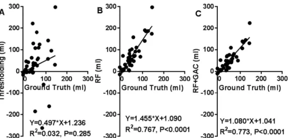
Fig. 6.The correlation between the automatically detectedΔCSF and the ground truth with thresholding (A), RF (B) and RF + GAC (C). The Pearson correlation coefficients werer= 0.178 (p = 0.285),r= 0.876 (pb10−6) andr= 0.879 (pb10−6) for thresholding, RF and RF + GAC, respectively. Compared to RF, the regression result of RF + GAC result is closer to the line of identity.

ground truth, with 1 indicating perfect similarity/overlap of the two techniques, and 0 indicating no overlap. We also calculated the Pearson correlation coefficients between the automatically detected CSF vol-umes,ΔCSF (between baseline and FU CT scan) with their correspond-ing ground truth (from manual delineation). The purpose is to evaluate the applicability of the proposed approach in processing both single scan and serial scans from the same patient.

3. Experiments and results

3.1. 10 fold cross-validation

We randomly divided the 38 subjects (26 from center A and 12 from center B) into 10 groups (2 groups having 3 subjects and 8 groups hav-ing 4 subjects) at baseline and FU separately. The randomly sampled Haar-like features from the training set were used to train the 10 RF classifiers (one for each group) in both baseline and FU. Exhaustive searches were performed tofind the optimal HU threshold to achieve the largest average DSC for baseline and FU scans, which were 25 and 23, respectively. Examples of automatically segmented CSF spaces by the HU thresholding, RF and the combined (RF + GAC) approaches on baseline and FU were given inFigs. 2 and 3, respectively. Qualitatively, the HU thresholding approach for CSF segmentation performed reason-ably well in baseline but poorly in FU scans when infarct-related hypodensity was present as a confounder. In baseline scans, the means and standard deviations of the DSCs were 0.676 ± 0.086, 0.728 ± 0.062, and 0.751 ± 0.059 for HU thresholding, RF and RF + GAC, respectively (Fig. 4A). The values in FU scans were

0.584 ± 0.151, 0.691 ± 0.077, and 0.721 ± 0.064 respectively for the three methods (Fig. 4B). With pairedt-tests, RF performed significantly better than HU thresholding in both baseline (pb10−4) and FU (pb 10−5). RF + GAC performed significantly better than RF in both baseline (pb10−3) and FU (pb10−5). The Pearson correlations between the au-tomatically detected CSF volumes with the corresponding ground truth are shown inFig. 5for these three methods. In baseline scans, the corre-lation coefficients werer= 0.774 (pb10−6),r= 0.946 (pb10−6) and r= 0.952 (pb10−6) for thresholding, RF and RF + GAC, respectively (Fig. 5A to C). In FU scans, the correlation coefficients werer= 0.447 (p = 0.005),r= 0.952 (pb10−6) andr= 0.951 (pb10−6) respectively for these three methods (Fig. 5D to F). The automatically detected CSF volumes from the two machine learning methods (RF and RF + GAC) had good correlations with ground-truth measures in both baseline and FU, but RF + GAC produced a slope closer to 1. For the analysis of changes in CSF volume in sequential scans, the Pearson correlation coef-ficients between the automatically detectedΔCSF and the ground truth werer= 0.178 (p = 0.285),r= 0.876 (pb10−6) andr= 0.879 (pb 10−6) for these three methods, respectively (Fig. 6A to C). As in the analysis of CSF volumes from single CT scans, the correlation of RF + GAC with the ground truth was closer to the line of identity than the one from RF alone.

3.2. Across center segmentation study

In order to demonstrate that our approach for edema quantification supports cross-center application, we used the 26 patients' CT scans ac-quired from center A as the training set and the CT scans of the

Fig. 8.The Dice similarity coefficients from thresholding, RF and RF + GAC from the cross-center analysis in baseline (A) and FU (B) scans (* indicating statistically significant difference). In baseline, the means and standard deviations were 0.673 ± 0.096, 0.730 ± 0.061, 0.758 ± 0.051 for thresholding, RF and RF + GAC, respectively. In FU, these values were 0.621 ± 0.102, 0.696 ± 0.072, 0.731 ± 0.061 for these three methods, respectively. RF performed significantly better than thresholding (p = 0.038 in baseline and p = 0.003 in FU) and RF + GAC performed significantly better than RF (p = 0.027 in baseline and p = 0.008 in FU).

remaining 12 patients from center B as the testing set. One example of automatically detected CSF space in baseline and FU with the proposed approach (RF + GAC) is shown inFig. 7. The means and standard devi-ations of DSC are shown inFig. 8, and the correlation between automat-ically detected CSF volume andΔCSF with the ground truth from RF + GAC are shown inFig. 9. In baseline scans, the means and standard deviations of DSC were 0.663 ± 0.107, 0.730 ± 0.061, and 0.758 ± 0.051 for HU thresholding, RF and RF + GAC, respectively (Fig. 8A). In FU, the means and standard deviations were 0.621 ± 0.102, 0.696 ± 0.072, and 0.731 ± 0.061 for these three methods (Fig. 8B). We found again that RF outperformed HU thresholding segmentation (p = 0.033 in baseline and p = 0.037 in FU) and RF + GAC outperformed RF (p = 0.027 in baseline and p = 0.008 in FU). The CSF volumes detected with RF + GAC were also significantly correlated with the ground truth mea-sures in baseline (r= 0.891, pb10−3), FU (r= 0.909, pb10−4), and ΔCSF (r= 0.844, pb10−3) (Fig. 9).

4. Discussion

In this study, we have developed and validated an automated ma-chine learning based approach for segmentation of CSF on serial CT im-ages of patients with hemispheric stroke. This approach allows accurate and rapid calculation ofΔCSF, a dynamic metric of cerebral edema. We have also demonstrated that our approach is versatile for the analysis of both single and serial CT scans from multiple stroke centers.

Our methods are different from previous image processing studies in stroke, which have largely focused on lesion segmentation using MRI during sub-acute or chronic stages. This study aimed to quantify the time-dependent evolution of cerebral edema by taking advantage of contrast provided by CSF as it shifts with increased intracranial pressure. Even though there are some lesion segmentation approaches using CT, which can be potentially adapted to our application, the lack of rigorous validation makes it difficult to predict the likelihood for success (Gillebert et al., 2014). Our approach shares some similarity to the pre-vious approaches which have utilized certain rules or features extracted from the image instead of relying solely on image intensity to perform segmentation (Matesin et al., 2001; Usinsskas et al., 2004, 2002). Some of these approaches might be incorporated into our learning based framework to unify the segmentation of edema and CSF, includ-ing the six Haralick features best describinclud-ing stroke and brain textures (Usinsskas et al., 2004) and histogram asymmetry between hemi-spheres (Maldjian et al., 2001). Likewise, we also adopted a machine learning approach for our task because we have demonstrated that CSF segmentation in CT scans of acute ischemic stroke patients is a more complex problem thanfinding an optimal threshold (even though head CT HU is an absolute measurement of the physical attenuation of a brain structure). RF has been demonstrated to be powerful in segmenting brain lesions with multimodal MRI images including T1,

T2, FLAIR and ADC at 3 months after stroke, which achieved a promising DSC of 0.60 ± 0.12 and significant correlation between segmented le-sion volume and the ground truth (Pearson correlation coefficient r= 0.76, pb10−4) (Mitra et al., 2014). In this study, we found that ad-dition of a GAC algorithm significantly improved overlap with ground truth CSF delineation compared with RF segmentation alone (i.e. higher DSC). RF and geodesic active contour complement each other well in CSF space segmentation. RF segmentation alone, though it can capture the CSF space globally, tends to over-segment CSF areas, which was se-quentially corrected by the geodesic active contour through locating nearby edges and removing false positive regions. As a result, we are able to achieve an average DSCN0.7 and close to line of identity in the correlation analysis of CSF volume andΔCSF. However, for practical pur-poses, the volumetric measurements of CSF obtained from the Haar-like feature based RF segmentation provided effectively as accurate quanti-tative results as those from the more computationally intensive sequen-tial GAC algorithm and may be adequate for analysis of cerebral edema from serial CT scans. GAC was able to further reduce false positive CSF regions as evidenced by improved DSC and a closer CSF volume to the line of identity when compared with the ground truth from manual delineation.

In this work, we chose to utilize CT instead of MRI for several rea-sons. CT's availability and imaging speed make it the ideal choice for ini-tial evaluation of stroke patients and detection of intracranial hemorrhage. CT also has less restrictive exclusion criteria compared to MRI, making it widely available (Rorden et al., 2012). CT has a much higher likelihood of serial imaging than MRI. The sequential CT changes after acute stroke reflects the underlying pathophysiological progres-sion from ischemic injury to infarction. Non-contrast CT follow-up re-veals infarct evolution, hemorrhagic transformation, cerebral edema and brain herniation (Nguyen and Mullins, 2006). By developing a reli-able automated segmentation tool, we can now perform large-scale studies to examine the dynamics of edema formation following ische-mic stroke, collected at multiple imaging centers. Indeed, we are plan-ning a large-scale study to examine genome-wide associations with our metrics of cerebral edema to discover novel genetic variants, genes and pathways that in_fluence the formation of edema.

In this study, we focused on segmentation of CSF rather than edema due to several complexities associated with the evolving hypodensity in brain CTs following ischemic stroke. Each 1% increase in tissue water leads to a decrease of 3 to 5% in X-ray attenuation and a decrease of 2.5 HU in CT, and hence edema contributes to hypodensity (Unger et al., 1988). However, infarcted brain tissue also becomes steadily more hypodense on CT (Vu and Lev, 2005). As a result, hypodensity results from a multitude of underlying causes, including edema, evolving in-farct, old lesions and leukoaraiosis, commonly seen in elderly patients (Vermeer et al., 2003). Therefore, CT hypodensity is a poor approxima-tion of edema, contaminated by infarcapproxima-tion and older lesions. It is known

that CT has limited ability to measure the size of early infarct (Saur et al., 2003) and CT hypodensity is insufficiently sensitive to quantify edema (Yoo et al., 2013).

In conclusion, we have validated an automated CSF quantification approach which is accurate and reliable, and can be applied to scans from multiple centers. CSF volume reduction may be a promising indi-cator of cerebral edema, because the CSF volume reduction is directly related to the increase in brain water resulting from cerebral edema, as described by the Monro-Kellie doctrine (Mokri, 2001).

Acknowledgements

The research was supported in part by the following grants from Na-tional Institutes of Health: 1R01HL129241 (to A.F.), 5K23HL129241 (to A.F.), 1R01NS082561-01A1 (to H.A.), R01NS084028 (to J.M.L.), R01NS085419 (to J.M.L.), P50 NS55977 (to J.M.L.) and UL1 TR000448.

I. F-C. is supported by the Miguel Servet programme (CP12/03298) Instituto de Salud Carlos III. C-C. is supported by NIH R01 grant, GENISIS project. Stroke Pharmacogenomics and Genetics Lab is supported by the Spanish stroke research network (INVICTUS), Generation Project (PI15/ 01978) and Pre-Test Stroke Project (PMP15/00022) Instituto de Salud Carlos III and Fondo Europeo de Deasarrollo Regional (ISCIII-FEDER). The Neurovascular Research Laboratory is supported by the Spanish stroke research network (INVICTUS), Pre-Test Stroke Project (PMP15/ 00022) and the European Stroke Network (EUSTROKE 7FP Health F2-08-202213) and Fondo Europeo de Deasarrollo Regional (ISCIII-FEDER).

References

Breiman, L., 2001.Random forests. Mach. Learn. 45, 5–32.

Caselles, V., Kimmel, R., Sapiro, G., 1997.Geodesic active contours. Int. J. Comput. Vis. 22, 61–79.

Dhar, R., Yuan, K., Kulik, T., Chen, Y., Heitsch, L., An, H., Ford, A., Lee, J.M., 2016.CSF volu-metric analysis for quantification of cerebral edema after hemispheric infarction. Neurocrit. Care. 24, 420–427.

Geremia, E., Clatz, O., Menze, B.H., Konukoglu, E., Criminisi, A., Ayache, N., 2011.Spatial decision forests for MS lesion segmentation in multi-channel magnetic resonance im-ages. NeuroImage 57, 378–390.

Gillebert, C.R., Humphreys, G.W., Mantini, D., 2014.Automated delineation of stroke le-sions using brain CT images. Neuroimage Clin. 4, 540–548.

Hacke, W., Schwab, S., Horn, M., Spranger, M., De Georgia, M., von Kummer, R., 1996. ‘Ma-lignant’middle cerebral artery territory infarction: clinical course and prognostic signs. Arch. Neurol. 53, 309–315.

Krieger, D.W., Demchuk, A.M., Kasner, S.E., Jauss, M., Hantson, L., 1999.Early clinical and radiological predictors of fatal brain swelling in ischemic stroke. Stroke 30, 287–292. Maldjian, J.A., Chalela, J., Kasner, S.E., Liebeskind, D., Detre, J.A., 2001.Automated CT seg-mentation and analysis for acute middle cerebral artery stroke. AJNR Am. J. Neuroradiol. 22, 1050–1055.

Matesin, M., Loncaric, S., Petravic, D., 2001.A rule-based approach to stroke lesion analysis from CT brain images. Image and Signal Processing and Analysis, 2001. Proceedings of the 2nd International Symposium on IEEE, pp. 219–223.

Minnerup, J., Wersching, H., Ringelstein, E.B., Heindel, W., Niederstadt, T., Schilling, M., Schabitz, W.R., Kemmling, A., 2011.Prediction of malignant middle cerebral artery in-farction using computed tomography-based intracranial volume reserve measure-ments. Stroke 42, 3403–3409.

Mitra, J., Bourgeat, P., Fripp, J., Ghose, S., Rose, S., Salvado, O., Connelly, A., Campbell, B., Palmer, S., Sharma, G., Christensen, S., Carey, L., 2014.Lesion segmentation from mul-timodal MRI using random forest following ischemic stroke. NeuroImage 98, 324–335.

Mokri, B., 2001.The Monro-Kellie hypothesis: applications in CSF volume depletion. Neu-rology 56, 1746–1748.

Nguyen, B.T., Mullins, M.E., 2006.Computed tomography follow-up imaging of stroke. Semin. Ultrasound CT MR 27, 168–176.

Rorden, C., Bonilha, L., Fridriksson, J., Bender, B., Karnath, H.O., 2012.Age-specific CT and MRI templates for spatial normalization. NeuroImage 61, 957–965.

Rosenberg, G.A., 1999.Ischemic brain edema. Prog. Cardiovasc. Dis. 42, 209–216. Rosenberg, G.A., 2000.Brain Edema and Disorders of Cerebrospinal Fluid Circulation.

Butterworth Heinmann, Boston.

Saur, D., Kucinski, T., Grzyska, U., Eckert, B., Eggers, C., Niesen, W., Schoder, V., Zeumer, H., Weiller, C., Rother, J., 2003.Sensitivity and interrater agreement of CT and diffusion-weighted MR imaging in hyperacute stroke. AJNR Am. J. Neuroradiol. 24, 878–885. Thomalla, G., Hartmann, F., Juettler, E., Singer, O.C., Lehnhardt, F.G., Kohrmann, M.,

Kersten, J.F., Krutzelmann, A., Humpich, M.C., Sobesky, J., Gerloff, C., Villringer, A., Fiehler, J., Neumann-Haefelin, T., Schellinger, P.D., Rother, J., Clinical Trial Net of the German Competence Network, S., 2010.Prediction of malignant middle cerebral ar-tery infarction by magnetic resonance imaging within 6 hours of symptom onset: a prospective multicenter observational study. Ann. Neurol. 68, 435–445.

Unger, E., Littlefield, J., Gado, M., 1988.Water content and water structure in CT and MR signal changes: possible influence in detection of early stroke. AJNR Am. J. Neuroradiol. 9, 687–691.

Usinsskas, A., Pranckeviciene, A., Wittenberg, T., Hastreiter, P., Tomandl, B., 2002. Auto-matic ischemic stroke segmentation using various techniques. Neural Network and Soft Computing, 2002. Springer, pp. 498–503.

Usinsskas, A., Dobrovolskis, R., Tomandl, B., 2004.Ischemic stroke segmentation on CT im-ages using joint features. Informatica 15, 283–290.

Vahedi, K., Hofmeijer, J., Juettler, E., Vicaut, E., George, B., Algra, A., Amelink, G.J., Schmiedeck, P., Schwab, S., Rothwell, P.M., Bousser, M.G., van der Worp, H.B., Hacke, W., Decimal, D., Investigators, H., 2007.Early decompressive surgery in malig-nant infarction of the middle cerebral artery: a pooled analysis of three randomised controlled trials. Lancet Neurol. 6, 215–222.

Vermeer, S.E., Hollander, M., van Dijk, E.J., Hofman, A., Koudstaal, P.J., Breteler, M.M., Rotterdam Scan, S., 2003.Silent brain infarcts and white matter lesions increase stroke risk in the general population: the Rotterdam scan study. Stroke 34, 1126–1129.

Vu, D., Lev, M.H., 2005.Noncontrast CT in acute stroke. Semin. Ultrasound CT MR 26, 380–386.

Yoo, A.J., Sheth, K.N., Kimberly, W.T., Chaudhry, Z.A., Elm, J.J., Jacobson, S., Davis, S.M., Donnan, G.A., Albers, G.W., Stern, B.J., Gonzalez, R.G., 2013.Validating imaging bio-markers of cerebral edema in patients with severe ischemic stroke. J. Stroke Cerebrovasc. Dis. 22, 742–749.