Learning Visuomotor Robot Control

Learning visuomotor robot control

THESIS

submitted in partial fulfillment of the requirements for the degree of

MASTER OF SCIENCE in

PHYSICS

Author : Frederik Hoekstra

Student ID :

-Supervisor : Prof.dr.ir. Tjerk Oosterkamp 2ndcorrector : Dr. Nanda van der Stap

Learning visuomotor robot control

Frederik Hoekstra

Huygens-Kamerlingh Onnes Laboratory, Leiden University P.O. Box 9500, 2300 RA Leiden, The Netherlands

April 13, 2018

Abstract

Deep reinforcement learning has solved the game of Go, along with all other board games. Can it also be applied to real-world use cases? This

research combines a literature study and experimental evaluation, focusing on the case of automation for tele-operated robotics. This is necessary because tele-operation of robots is slow and cumbersome. Classical robotics solutions are expensive, and limited in precision, but

Contents

1 Introduction 1

2 Literature Methods 5

3 Theory 7

3.1 Research questions 7

3.2 Introduction to Deep Learning 7

3.2.1 Short history 7

3.2.2 Multi-layer perceptron 8

3.2.3 Convolutional Neural Networks (CNNs) 9

3.2.4 Unsupervised Learning 11

3.2.5 Overfitting 13

3.3 Reinforcement Learning 14

3.3.1 Policy 15

3.3.2 Q-function 16

3.3.3 Model (transition function and reward function) 17

3.3.4 Value function 17

3.4 Learning from demonstrations 19

3.5 Meta-learning and transfer learning 20

3.6 Conclusion 21

4 Experimental Methods 23

4.1 Guided Policy Search 23

4.1.1 Trajectory Optimization 24

4.1.2 Neural network architecture 24

4.1.3 Memory States in Guided Policy Search 26

5 Experiments 29

5.1 Box2D inverse dynamics 29

5.2 Network architecture comparison 39

5.3 Box2D peg insertion 40

5.4 3D 7-joint robot arm inverse kinematics 45

6 Discussion 51

7 Conclusion 55

Chapter

1

Introduction

The Problem

Sub-sea, a building that is on fire or at the verge of collapsing due to an earthquake, space. These are hazardous environments where remotely-operated robots are necessary. Robots have been doing manufacturing work for decades, and right now, the technology is there to make them more capable so they can be used to save lives in these strenuous and unknown environments. This requires a number of solutions which are studied under the i-botics program at TNO, where I did this internship.

The goal of the i-botics project is ”...to provide the human operator with full perceptual and manipulation capabilities to intuitively perceive the remote environment and act as if being present at the remote site. ” [1] One of the problems is latency: actions of the operator arrive at the robot after some lag time T1, and information about the environment of

the robot takes another period T2to reach the operator. This makes

com-plex interactions at large distances awkward and may cause instability of the system when using feedback control schemes. Automation of such interaction is non-trivial due to the variance of tasks.

The goal

The state of Deep Robotic Learning

As an example of a task, let’s say we want to automate turning a screw. A traditional robotics approach to this problem would be: write a screw-localizer module, then use an inverse dynamics module and trajectory planner to move the robot arm to the correct position, then use sensors to determine if the screw was grasped, and if not retry, until the screw is grasped, then turn it. All of these modules traditionally require a lot of programming and/or expensive sensors. This is called the robot control pipeline [2].

Deep Robotic Learning is the science of incorporating artificial neural networks in the robotic pipeline. Artificial neural networks have radically improved automatic image classification [3] [4] [5], and more recently rev-olutionized reinforcement learning [6]. The ability of a neural network to learn a generalizable function from training is exceptionally useful in robotics.

A task that has been widely studied in Deep Robotic Learning research is grasping [7] [8] [9]. Convolutional Neural Networks are very good at image classification, and can combine image input with other modalities. This has been leveraged by the robotics field, where the neural network is used as a grasp success predictor or GQ-CNN (Grasp Quality Convo-lutional Neural Network). These methods require an enormous amount of samples [8] [7], but the interest in grasping research has also led to the Dexnet databases with objects and optimal grasps[10][11][12], which can be used to train a GQ-CNN without needing thousands of hours of robot time (and wear and tear).

However, a GQ-CNN can only do that: predict a grasp quality based on input from a depth sensor. There are many more tasks that robots do that would benefit from automation, and just training a network from a database is relatively simple. So we looked for a different method for more general robotic automation.

3

solution to this problem is proposed in [13], where a neural network learns the entire distribution of actions for a given input. Their neural network also integrates vision input and a recurrent (memory) element, which al-lows it to remember what it has previously experienced during a rollout, so it can remember its choices (e.g. front or side approach). With demon-strations, the number of samples is relatively low compared to GQ-CNNs. It is hard to train a vision network with such limited samples. Their so-lution is to use an auto-encoder (see Section 3.2.4). This means, however, that only features that take up a significant portion of the pixels in the input, are ’sensed’ by the network. Even though the sample count is rel-atively low for vision Deep Learning, it is still too high for an actual ap-plication: they used multi-task training on 5 tasks and gathered 15 hours of demonstration data for 5 tasks (success rates on all tasks in excess of 75%). Their performance for only 3 hours training on a single task are at best 44%. This means that 15 hours (or a comparable number) of training data is necessary to learn a robust network, and you cannot successfully train for a single task using only 3 hours of demonstrations. 15 hours of human demonstrations is not financially viable for most applications.

Research question and overview

The main research questions are”Can Deep Reinforcement Learning be used to automate tasks in real-world robotic applications? To which extent? What are its requirements? What are its strengths and weaknesses?”. To answer these ques-tions, a literature study was conducted and experiments were performed on a subset of the algorithms. The methods of the literature study are de-scribed in Chapter 2. The methods used in the experiments are explained in Chapter 4

The questions answered with the literature study in Chapter 3 are

Which kinds of Deep Reinforcement Learning algorithms are available? What is their sample efficiency? Which algorithms have been used successfully in robotics and which functionality do they provide?.

The experiments that were carried out answer the following questions:

Can a neural network learn a vision-based policy for moving a heavy 2-joint arm to 1 of 2 target positions by applying torques in a 2D environment that generalizes to different initial positions? How do choices in number of layers and pre-trained visual processing in the neural network architecture affect the performance of the policy network? Can a neural network learn a torque-based policy for 2D peg insertion? Can a neural network learn a policy for moving a 7-joint arm to a commanded target position in a 3D environment using joint velocity commands?

Descriptions of the experiments can be found in Chapter 5, along with their results.

Chapter

2

Literature Methods

The questions I wanted to answer are: Which kinds of Deep Reinforcement Learning algorithms are available and what is their sample efficiency? Which algorithms have been used successfully in robotics and which func-tionality do they provide?

I started my search using the search terms in the left column of Table 2. I searched the Leiden Univsersity Library Catalogue and Google (Scholar). Another starting point of my search was the work of Levine’s group in Berkeley, specifically [2]. Using the papers I found, I continued my search with the terms in the second column of Table 2.

Initial Derivative

Deep Reinforcement Learning Grasping

Deep Robotic Learning Grasping Quality

Reinforcement Learning GQ-CNN

Guided Policy Search Q learning Value learning

Chapter

3

Theory

Introduction

The goal of this theory section is twofold: on the one hand, it introduces the reader to Deep Learning and Reinforcement Learning. It also answers the research questions of the literature study.

3.1

Research questions

Which kinds of Deep Reinforcement Learning algorithms are available? What is their sample efficiency? Which algorithms have been used suc-cessfully in robotics and which functionality do they provide?

3.2

Introduction to Deep Learning

3.2.1

Short history

Neural networks were first invented in the 1950s in an effort to replicate the low-level functionality of the brain by mimicking a network of neu-rons. These were called multi-layer perceptrons, and are also called ’fully connected layers’ when incorporated into a larger network architecture.

The first network that was applied to a real-world problem was MADA-LINE, a three-layer perceptron. It was used to filter echoes from phone sig-nals, and implemented in hardware with vacuum tubes and memistors[14].

Figure 3.1:Multi-layer perceptron network and neuron function diagrams.[18]

by proving that a single-layer perceptron cannot learn an XOR-function. Multiple layers with non-linear activation functions can learn that, but this was not widely known, and there was no learning algorithm for such a network.

Thus the ’XOR argument’ spread, and as a consequence, funding was withdrawn and the research ceased.

The second deep learning revolution happened in the 80s. A new learning rule for multi-layer perceptrons was popularized: backpropaga-tion [16]. This allowed the error of the output neuron to be backpropa-gated through multiple layers of a network to update all weights accord-ingly. This made it possible to have a network learn the XOR-function. In a regular MLP, every input scalar would need its own unique associated weights: this is problematic when processing large images or other high-dimensional data. In 1989, Lecun et al. [17] invented a convolutional neu-ral network: a special kind of architecture with only local connections and weight sharing which makes it very suitable for image processing. This is the building block that would later allow neural networks to process arbi-trarily large images, or other locally correlated input such as speech and time series data. Throughout the 1990s and early 2000s, neural networks lost popularity, but in the last decade, deep learning has gained popular-ity due to the availabilpopular-ity of big data and computing power in relatively cheap Graphical Processing Units, and a host of new architectures, some of which are explained in section 3.2.4.

3.2.2

Multi-layer perceptron

3.2 Introduction to Deep Learning 9

produce an output, which is passed along to all m neurons in the next layer [19]. The output of a single neuron is thus: y= f(∑_iwixi+b)

The inputs, summation and output represent the dendrites, soma and axon of biological neurons.

During training, the weights are updated according to the following update rule:

wnew =w+η(t−y)·x (3.1)

with x the input vector, w the weights vector, y output, t target (desired output).

Instead of using the error (t−y) directly, a loss function is usually defined to map the output vector to some scalar error. For example, a re-gression task would typically use a mean square error (MSE) loss function.

3.2.3

Convolutional Neural Networks (CNNs)

For this explanation, I will assume that the input to a convolutional layer is an RGB image: this could of course also be a higher or lower dimensional input. Convolutional layers work by sharing the same weights all over the image, making them translation-invariant. The weights are stored in filters, or local receptive fields[19]. A filter has a dimension of f ∗ f ∗d, wheredis the depth of the input image (3 for an RGB image), and f is the filter size, a number usually much smaller than the size of the input image. Thus, the convolution is usually only applied in the spatial direction.

cm,n =

k,l=Fe,eF

∑

k,l=−Fe,−Fe

wk,lxm+k,n+l (3.2)

The output at the m,n position is the product of the filter with the input pixels in a small (filter size) region around the m,n position in the input.

Every filter in the layer convolves separately with the input to create a different (grayscale) feature map. These feature maps together form the input image to the next layer: the depth is now the number of filters in the previous (input) layer.

3.2 Introduction to Deep Learning 11

and strides, including the arithmetic for transposed convolution (a similar inverse-like operation which creates a larger output image).

Max-pooling is often used in-between convolutional layers to shrink the height and width of the feature maps and to reduce the number of parameters. Max-pooling of sizenis an operation with an output half the height and width of the input. This is done by dividing the input inton∗n

blocks; then for each block, the maximum value is set as output. This is done separately for each feature map, so depth is preserved. Thus, spatial information is lost, while depth (feature information) is preserved: this is desired for classifier networks, but not for robot control, where position information is more important, and less feature information is necessary than for classification. Section 4.1.2 contains information about convolu-tional neural network architectures used for robot control.

3.2.4

Unsupervised Learning

In the previous examples, training a neural network was done by present-ing it with trainpresent-ing examples consistpresent-ing of input and the correspondpresent-ing desired output. This is calledsupervised learning. However, most real data is unlabeled: when there is no label, we cannot do supervised learning.

There are a few things that one can do with unsupervised learning in combination with neural networks: learning a low-dimensional encoding of high-dimensional data such as images [22], training a generator for syn-thesizing real-looking data [23], using unlabeled data to aid in training a classifier [24].

For dimensionality reduction, an autoencoder is typically used: a con-volutional network can serve as an encoder. It transforms the input data into a latent vector of reduced dimension. This latent vector is then fed into the decoder: a deconvolutional network, essentially the inverse of a convolutional network that tries to reconstruct the image. (the values of the weights are not forced to be related to those of the encoder though). The error is then the deviation from the input image. Due to the shape of the network diagram, an autoencoder is sometimes called a diabolo net-work [25].

The other popular deep unsupervised learning technique is called Gen-erative Adversarial Networks (GANs) [23]. A GAN also typically consists of a convolutional and a deconvolutional network. In this context, the de-convolutional network is thegenerator: it generates high dimensional data using a random latent vector as input. The convolutional network is the

Figure 3.3: Autoencoders encode and decode an input, and aim to minimize the reconstrution loss[21].

3.2 Introduction to Deep Learning 13

Figure 3.5:Fake celebrity images generated by a GAN. This GAN was trained by

gradually adding layers and scaling up the resolution during training [27].

data or from the generator. In a GAN, the generator is rewarded for fooling the discriminator: thus it learns to generate output that the discriminator cannot distinguish from real.

This technique can be used to generate images and other high dimen-sional data, based on an unlabeled dataset. Notable examples include Image-to-Image translation [28] [29] and speech synthesis [30], a well as the celebrity face generator [27] (see Figure 3.5).

Both auto-encoders and GANs can be used to aid training of a classifier when using a big unlabeled and a small labeled dataset [24]. Learning an encoder is a similar task to learning a classifier: there is commonality in learning common patterns in the input data and encoding the differences between samples: this aids both reconstruction and classification. A dis-criminator is also similar to a classifier: the classes is separates are simply ’all the real classes’ and the ’fake class’.

3.2.5

Overfitting

Neural networks typically have millions, or tens of millions of parame-ters. Thus, overfitting is a major problem, especially with larger networks and/or smaller datasets. There are multiple techniques which can be used to prevent overfitting.

using batch normalization between convolutional layers (see section 4.1.2). Other ways to prevent overfitting address the dependency of the network on a limited number of weights. Dropout [32] is one such method, where a fraction (usually 0.5) of the connections in the network are removed dur-ing traindur-ing. Finally, a penalty can also be set on havdur-ing some very strong connections by adding a regularization term to the loss function of the form∑iw2i wherewi are the weights of the network.

3.3

Reinforcement Learning

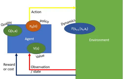
Figure 3.6: The setup of Reinforcement Learning. An agent interacts with the

environment, sending actions and receiving observations and rewards. The ovals are functions: the policy, which selectst an action based on an observation, the quality assigns a score (expected future reward) to an action in a certain state, and the value function specifies the expected future reward for the state. The dynamics, which determine the likelihood that a state will follow from a previous state and action, can be modeled by the agent to perform planning.

Reinforcement Learning is a class of problems which revolves around an agent choosing actions to maximize the sum of received rewards from the environment: in short, sequential decision-making. The basic model in the theory of reinforcement learning is the Markov Decision Process (MDP): the probability to transition from statest tos0_t+1is only dependent

3.3 Reinforcement Learning 15

the observation is not the full state, it is called a Partially Observed Markov Decision Process (POMDP).

At every timestep t the agent receives an observation ot and reward

rt from the environment, and processes those to take an action at. The

objective to maximize is the sum over all rewards ∑_t(rt). Sometimes the

word cost function is used instead of reward, they are the same thing, but with opposite sign.

The key concept of reinforcement learning is sequential decision-making. Although I will mainly talk about Deep Reinforcement Learning in this section, reinforcement learning is a field that is much older than deep neu-ral networks.

However, there are some functions in reinforcement learning that can be approximated by neural networks. Instead of listing a number of al-gorithms, I would like to focus on the relevant functions and explain how they are used in recent papers in Deep Reinforcement Learning, namely: the policy in section 3.3.1), the Q-function in section 3.3.2, the model in sec-tion 3.3.3, and the value funcsec-tion in secsec-tion 3.3.4. After that, I will look at 2 specific solutions to the sample-efficiency problem in robotic deep learn-ing: learning from human demonstrations in section 3.4 and meta-learning (from simulations) in section 3.5.

Note that reinforcement learning is a very old research area, and all of these concepts have been around since the 1950s [33]. The only thing that is new is the use of deep neural networks in this context.

3.3.1

Policy

πθ(at|ot)orπθ(at|st) (3.3)

The policyπis the distribution over actionsat, given an observationot (or

the full state st). The policy is defined by the parameters θ. This is the

function that represents what the agent is likely to do given an observa-tion.

A variation on the above definition that is often used is to implement a recurrent network as a policy: a network that receives not only the input at each timestep, but also has a memory which can be written to and read from. The disadvantage is that a recurrent neural network is effectively an extremely deep network and usually requires more samples.

The simplest reinforcement learning algorithms are policy gradient meth-ods. They sample from the (noisy) policy and then directly update the policy parameters θ by gradient descent on the objective. The first such

A new, very sample-efficient policy search method is called Guided Policy Search [35] [2] [36] [37] [38]. This method uses optimization in ac-tion space of very simple local linear-Gaussian controllers. These local controllers consist of a linear feedback and feedforward term (plus Gaus-sian noise) at every timestep and can thus only learn a fixed sequence from point A to point B. However, for Guided Policy Search, the network tries to learn a policy function that behaves similarly to these trajectories, and then the local controllers adapt to and improve upon the network’s behaviour. A fit of the dynamics can be used for faster optimization of the local controllers. This is the most sample-efficient end-to-end learning method available for deep reinforcement learning. For more information on Guided Policy Search, see section 4.1.

3.3.2

Q-function

Q(st,at) (3.4)

The Q-function assigns a ’quality’ to state-action pairs and can be used to decide which action is most likely to eventually lead to a high cumula-tive reward.

The basic Q-learning update rule is:

Q(st,at) = (1−α)Qold(st,at) +α·(rt+γ·maxaQ(st+1,a)) (3.5)

Here, the learning rate (step size) isα, st,at,rt are state, action and reward

respectively, at timestept, andγ is the discount factor. This is a factor by

which future rewards are discounted: this is the same factor that is used in finance when calculating future expected profits. Future rewards are uncertain and thus are worth less than the same reward now.

This update rule, however, assumes that the next action will be the one with the highest Q-value. However, a policy that would always do that would never explore other actions. This is at the heart of the exploration-exploitationproblem: a balance needs to be struck between exploiting what the agent knows will work and exploring new actions. Other words used in this context arevariance for an algorithm with a lot of exploration and

bias for an algorithm that does more exploitation. Q-learning is usually done with an epsilon-greedy policy: take the optimal action with proba-bility(1−e), take a random action with probabilitye.

If we change the update rule by taking into account the actual next action that the agent has taken, instead of assuming it will always take the optimal action, it will lead to:

3.3 Reinforcement Learning 17

This update rule is called SARSA [39], because it takes those 5 parameters as input:St,At,Rt,St+1,At+1.

A recent Deep Learning example where the Q-function was represented by a network can be found in [40], where a neural network learns to play Atari games. The input is the state of the pixels, and the outputs are the Q-values for all the possible actions. This network achieved superhuman performance on Breakout, Enduro and Pong. But not on Q*bert, Seaquest and Space Invaders.

In Robotic Deep Learning, the classifying power of convolutional neu-ral networks is used to classify potential grasps on depth image data [8] [10] [11] [12]. This is called a grasping quality convolutional neural net-work (GQ-CNN). In an application, this netnet-work is presented with several hundred grasp candidates, it assigns a grasp quality to each of them, then the robot executes the grasp with the highest quality. This is an example of a Q-function for a discrete action space of grasp candidates.

3.3.3

Model (transition function and reward function)

dynamics/transition: p(st+1|st,at)orst+1= f(st,at) (3.7)

reward: rt+1 =g(st,at) (3.8)

A model approximates the environment: based on the current state and action, it returns (the probability distribution over) the next state, and sometimes the reward function is also modeled.

The advantage of fitting a model is increased sample efficiency: less samples are needed if you use the gathered information to infer a model. The disadvantage is that the performance of the learned policy is limited by the accuracy of the model. This is very important in Robotic Learning, as taking samples with an actual robot is time-consuming, and learning in simulation usually does not transfer easily to real environments [41]. When tens of thousands of samples can be taken using simulation, model-free is the way to go, as it allows for more complex tasks to be learned [37].

3.3.4

Value function

The value function represents the expected cumulative reward from a given state, using the policy and an estimate of the dynamics. Given the Q-function, we can say that:

The foundation of Value learning is the Value Iteration algorithm as developed by Bellman[33]. This algorithm requires a transition function

p(st+1|st,at) and a reward function r(st,at,st+1 and is thus model-based.

The algorithm is described in pseudocode in Algorithm 1.

Algorithm 1The Value Iteration algorithm

Require: Sset of all states;Aset of all actions;λthreshold

Require: P(s0|s,a)transition function andR(s,a,s0)reward function 1: AssignV0(S)arbitrarily

2: k ←0 3: repeat

4: k← k+1

5: for allstatess∈ Sdo

6: Vk(s) = maxa∑s0P(s0|s,a)(R(s,a,s0) +_γV_k−1(s0)) 7: end for

8: until|Vk(s)−Vk−1(s)| <λ∀s

9: return Vk

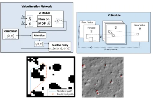
Tamar et al.[42] developed a neural network implementation of this Value Iteration algorithm to learn to plan (see figure 3.8). To do this, they implemented a neural network architecture that includes the reward and transition function (see Section 3.3.3), as well as an iteration module that refines the value function, and a policy. They applied this algorithm to a grid-world, a crater landscape, web search and a simple continuous con-trol obstacle avoidance task. Note however, that this method assumesfully observableMDPs, and does not cover the case of partial observability.

3.4 Learning from demonstrations 19

Figure 3.7:The Value Iteration Network. All functions are implemented as neural networks: reward fR, dynamics fP, Q-function, Value function and policy. Top

left: the full network. Top right: The Value Iteration module. The iterative nature of this algorithm is implemented using a recurrent neural network. Bottom: the environments that this method was applied to: grid world and Mars. Note that this method assumes full observability.

agents introduces enough variance to counter the inherent bias of actor-critic methods [43]. Sample efficiency is thus better than most value and Q-learning methods, but still orders of magnitude behind Guided Policy Search.

The difference between the definitions of the Q and Value functions may seem small and trivial. The difference between Q-learning and Value-learning algorithms, however, is not small and trivial: Q-Value-learning algo-rithms work by trial and error and are model-free. Value learning algo-rithms are generallymodel-based.

3.4

Learning from demonstrations

an additional input that is dependent on the state of the network in the previous timestep. They used a one-hot vector to do multi-task training: a vector of zeros with a 1 in a single dimension to indicate which task is being performed. See section 1 for more about this paper.

A standard improvement on this method for reactive (non-memory) policies is DAgger [44]. This involves doing a roll-out of the policy, then annotating the new inputs that are received with appropriate outputs. This is useful, since a trained reactive policy may not exactly follow the demonstrated trajectory, and instead encounter inputs that are outside the distribution of demonstrations.

Another way in which demonstrations can help is by providing a start-ing point for Guided Policy Search. This is especially useful when usstart-ing a model-free optimizer [37]. For more information on Guided Policy Search, see section 4.1.

The most sample-efficient way of doing demonstration learning is Guided Cost Learning [45]. This Inverse Optimal Control method uses Guided Policy Search, and optimizes a cost function that is represented by a neu-ral network at each iteration. In this way, it adapts the cost function so that it not only encodes the right information for a successful policy, but is also easily learnable at each iteration of policy optimization.

3.5

Meta-learning and transfer learning

Gathering a lot of samples is easy in simulation. This is an important rea-son why deep reinforcement learning is so successful in games, but not so much in robotics: the real world is different from simulations in ways that are important for robotic task execution. There is a number of ways to improve the transfer of simulation learning to the real world.

The CAD2RL algorithm [46] uses a number of simulation environments with different colours and rendering settings. A policy is trained for col-lision avoidance of a drone in these very different looking environments. The trained policy can then be deployed to a real drone, since the real world looks like ’just another simulation’. The diversity in the synthetic environments is apparently good enough so the policy can generalize to the real world.

3.6 Conclusion 21

instead of searching for the parametersθthat deliver optimal average task

performance, we are looking for the parameterseθthat deliver optimal task

performance after 1 gradient step update for that specific task. As such, it finds a point in parameter space from where it can quickly learn all of the trained tasks with just 1 (or a few) steps. This allows it to generalize to new tasks.

As such, MAML could be used to train a policy network on a lot of dif-ferent simulation environments, which could then quickly learn a similar policy for a real robot.

Figure 3.8:The MAML [47] algorithm optimizes for performance after 1 gradient step. As such, it finds a point in parameter space from where it can quickly learn all of the trained tasks with just 1 (or a few) steps. This allows it to generalize to new tasks. Figure from [47].

3.6

Conclusion

Learning from demonstrations is possible, using an LSTM that learns the entire distribution of human actions, however this requires 15 hours of hu-man demonstrations and has not been shown to work with a sophisticated vision architecture, only with an autoencoder (which can only learn to see large objects)[13]. Model-free Deep Reinforcement Learning algorithms perform best, but they need lots of samples and are thus only suitable for use in simulated environments.

The easiest robotics application of Deep Learning is Grasping Qual-ity Convolutional Neural Networks (GQ-CNNs), which rate grasp can-didates based on RGB-D image data. Training can be performed using synthetic data, thus sample-efficiency is not an issue. Implementation of such a method on a grasping robot arm would be straight-forward.

similar and/or simple tasks. Another option is pre-training in simulation: this works best with meta-learning, since the simulation is likely different form reality: training a network to adapt easily to different simulations could allow it to work well in the real world too.

Chapter

4

Experimental Methods

This chapter consists of an explanation of the Guided Policy Search algo-rithm and some of its extensions in Section 4.1, and an exposition of the methods and materials in Section??, including software and hardware.

4.1

Guided Policy Search

Guided Policy Search is a family of algorithms that use Linear Gaussian state-feedback controllers (which are in this context referred to as trajecto-ries) to guide a neural network in learning an optimal control policy.

Overview

There are different local controllers for differentconditions: different con-ditions are typically defined by different initial and/or target positions. Thus each controller learns a sequence of actions and feedback terms to reach a different target state.

A single neural network is then trained to imitate these local controllers: for each timestep, the neural network input and the local controller’s out-put have been stored, and the network is trained through regression to return an output similar the actions that the controllers.

this roll-out by limiting the KL-divergence between the trajectories and the network’s global policy.

If no network is used, the trajectories are constrained to their previous roll-out.

The parameters of a trajectory include a feedback term and a forward action term at each timestep.

The parameters of the trajectory can be optimized in a variety of ways, with model-free updates, model-based updates, or combining both kinds of updates. [38] This is discussed in Section 4.1.1

4.1.1

Trajectory Optimization

The standard trajectory optimizer is the iterative Linear Quadratic Regulator[49]. This method is based on a linear fit of the local dynamics of the system, and a quadratic expansion of the cost function. Then, the cost is mini-mized, constrained to a certain KL-divergence, since the first and second-order approximations are only valid close to the trajectory. For details, see [35]. Another optimizer is the path integral-based PI2 optimizer [37], which is stochastic. The lack of a dynamics fit means this optimizer is slower, but can learn more complex actions because it is not constrained by any assumptions about the dynamics of the system being linear and smooth. This can be useful for tasks like door opening.

A third option is to combine the model-based LQR update with the PI2 model-free update, which is done in the PILQR optimizer [38].

4.1.2

Neural network architecture

The neural network architecture used is a fairly straight-forward convolu-tional neural network that receives the image as input. Its output is then concatenated with robot state information (joint angles and speeds), and passed through 2 fully connected layers with 40 hidden units. The output layer consists of 7 nodes, the number of joints of the robot arm. All activa-tions are ReLu (rectified linear unit f(x) = xif x>0, else 0) except for the output layer, which is linear.

Batch normalization

4.1 Guided Policy Search 25

input to those layers changes drastically due to weight updates of earlier layers, their own weights will have to be adjusted to handle this different input. It also reduces sensitivity to initialization.

Soft-argmax

Most convolutional neural networks transform an input image with large spatial dimensions and low depth to a feature vector where all spatial in-formation is lost and only feature inin-formation is left.

However, for control tasks, it is important to keep the spatial informa-tion. It is still desirable to reduce the size of the output of the convolutional layer, to reduce the number of weights in the fully connected layers. This is why the feature maps of the last convolutional layer are passed through a soft-argmax layer to extract the positions of the highest activation for each feature. First, a spatial softmax is applied to the input acij, then the

expected position(fcx, fcy)is calculated as the mean of this softmax

distri-bution:

scij =eacij/Σi0_j0eaci0j0

fcx =Σijscijxij (4.1)

fcy=Σijscijyij

Supervised and unsupervised pre-training

In order for the policy network to learn a controller, the vision layers must be pre-trained to learn the features of relevant objects. There are 2 ways to do this: supervised or unsupervised.

For supervised pre-training, a dataset of images with position labels is used: position labels can be positions of parts of the robot and/or target marker/object. Add 1 fully connected layer behind the soft-argmax for rescaling.[2]

For unsupervised pre-training, no labels are used. Instead the network is set up like an autoencoder, where the target output is a down-sized grayscale version of the input image. The network learns to ’reconstruct’ this image by applying 1 fully connected layer to the output of the soft-argmax layer. In order to make sure that the network learns the posi-tions that are useful for predicting the dynamics, a smoothness penalty is added to the loss function: gslow(ft), the L2-norm of the second time

gslow(ft) =||(ft+1−ft)−(ft−ft−1)||2

L =

∑

t,k

||Idownsamp,k,t−hout(fk,t)||2+gslow(fk,t) (4.2)

The unlabeled dataset can be generated simply by training a trajectory on a task with constant target and initial position. The trained feature extractor can then also be used to translate images into feature coordinates, which can be used as state variables for cost functions and trajectories.[36] In other words, it allows trajectory training on tasks that require visual position information. An image can then be used to define a target state.

4.1.3

Memory States in Guided Policy Search

Guided Policy Search has mostly been used to train a reactive policy: a function from observation to action, independent from previous timesteps. Some tasks however, require memory. These are often trained using a re-current network: a network with layers that receive inputs from the state of the network at the previous timestep. However, this effectively makes the network as deep as the number of timesteps and makes a lot more difficult to train than a reactive policy.

In [51], an extension of Guided Policy Search is proposed and proven to work using memory as part of the state. In this work, a number of state (and observation) dimensions have been added, with numbers that can be directly modified by the policy using additional action dimensions. By separating the memory from the policy, the policy is effectively still reactive. The only difference is that it now also learns to write to and read from the memory.

4.2

Experimental methods and materials

The experiments were done by applying variations of the Guided Policy Search [52] algorithm to different experiments in 2D (using Box2D [53]) and 3D (using Gazebo [54]) simulation environments.

Experiments were designed to test whether the system could learn policies that need to estimate:

• (local) inverse dynamics for 2D

4.2 Experimental methods and materials 27

• strategies for 2D peg insertion (non-linear dynamics)

Experiments consist of a number of conditions, which typically have different initial and/or target positions. Each sample is 5 seconds, each timestep 0.05 seconds for a total of 100 timesteps per sample.

For every experiment, the MDGPS algorithm[55] is used, the network receives the joint angles, joint velocities and end effector position as in-put. Comparisons are made between the performance of the network as a function of additional input. In these comparisons,tgtstands for direct target position input;imgmeans image input from which the target posi-tion can be inferred;blindnetworks have no target information, only pose information.

The 2D environment was used to compare the performance of different network architectures.

For all vision experiments, the convolutional layers of the network are pre-trained on pose and target position estimation from images. All net-work optimization uses the Adam [56] optimizer.

The software I used consists of the Guided Policy Search repository [52], which is implemented in Python 2.7 [57] and uses the Tensorflow [58] li-brary for deep learning. This was run on Ubuntu 16.04 LTS.

Among the modifications I made to the Guided Policy Search reposi-tory are: image input for Box2D; efficient storage of image data in sample objects; an upgrade from tensorflow 0.8 to tensorflow 1.3, which adds new functionality and compatibility; extensive neural network architecture op-tions throughhyperparams.py; improvements to interfacing with Gazebo.

m

Hardware used:

CPU Intel(R) Core(TM) i7-6700K CPU @ 4.00GHz

Motherboard ASUS MAXIMUS VIII RANGER

RAM 2x8GB 2133MHz DIMM

GPU Nvidia GeForce GTX 970 4GB

Chapter

5

Experiments

In this chapter, the performed experiments are described for the 2D and 3D simulation envrionments. Sections 4.1-4.4 are built up as follows: each section starts with the respective research questions, then the hypothesis is stated, followed by the specific methods used in the experiment. The results are then presented, and the conclusion answers the research ques-tion.

5.1

Box2D inverse dynamics

Research Questions

Can a neural network learn a vision-based policy for moving a heavy 2-joint arm to 1 of 2 target positions by applying torques in a 2D environ-ment that generalizes to different initial positions? How does a vision-based network compare to a blind network, and a policy network that receives the exact target position directly?

Hypothesis

Methods

We use the Box2D [53] environment with a heavy 2-joint arm and weak motors. The target is marked by a blue star figure at a distance (x,y) of

(10, 5)or(10,−5)from the base of the arm. Both arm segments are length 10.

The vision network has 3 convolutional layers followed by a soft-argmax layer and then 3 fully connected layers and is pre-trained on images of random target and arm positions to estimate the target position. The net-work’s square filters have sizes 7,5,5, the first conv layer has a stride of 2, and the activations are all ReLu, excrept for the last layer which is linear.

The policy network that receives the joint state and end effector po-sition, along with the optional target input, consists of 2 fully connected hidden layers of 20 units with ReLu activations, the final layer has a linear activation function.

Initial positions of the robot arm are shown in figure 5.1, figure 5.2 and in table 5.1 as defined by the joint angles in radians: angle 1 is 0 if the first segment of the arm points straight up, and the positive direction is anti-clockwise. angle 2 is 0 if the second segment is aligned with the first, also anti-clockwise.

The trajectories (Linear Gaussian Policies) for each training condition are pre-trained with 5 iterations of LQR, taking 3 samples per condition per iteration. Guided Policy Search training was done using the Mirror-Descent Guided Policy Search algorithm for 4 iterations with 3 samples per condition per iteration.

The cost function used consists of 3 terms: a small cost on the square magnitude of the action vector to punish unnecessary and high forces, an L1L2 norm on the end effector distance of the following form: L =

0.5l2d2+l1

√

α+d2 whose weight increases quadratically with the time

since the start of the trial, and a binary cost term for the end effector dis-tance at the last timestep.

5.1 Box2D inverse dynamics 31

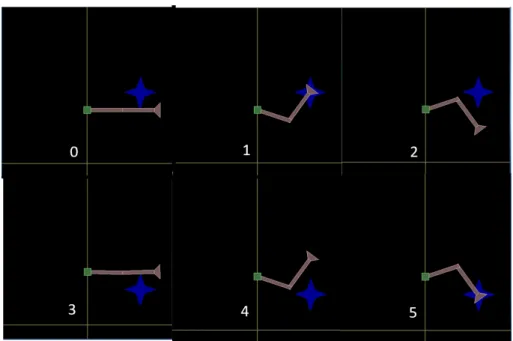
Figure 5.1: Train conditions for the 2-joint arm Box2D environment. The arm is shown in the initial pose, the target position is marked by the blue star and the condition number (index) is shown in white. The yellow lines intersect at (0,0), the green base of the arm is at (0,15).

Condition number Training Test

for (high, low) target positions

joint angles (a1, a2) inπradians

0, 3 -0.5, 0

1, 4 -0.6, 0.4 -0.6, 0

5.1 Box2D inverse dynamics 33

Results

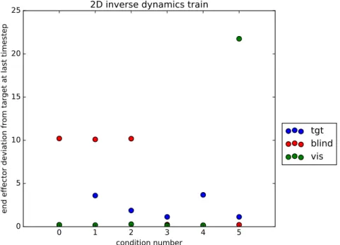
0 1 2 3 4 5 condition number

0 5 10 15 20 25

end effector deviation from target at last timestep

2D inverse dynamics train

tgt

blind

vis

5.1 Box2D inverse dynamics 35

1 2 4 5

condition number 0

2 4 6 8 10 12

end effector deviation from target at last timestep

2D inverse dynamics test

tgt

blind

vis

Conclusion

As expected, the vision-based policy network’s performance exceeds that of the blind network, which has learned a mapping from initial to target position that, given our train and test conditions, can only be right for half the conditions: there are 2 different target positions but the blind policy receives the exact same input regardless of target position so it can, at best, learn to move toward one target position.

The vision-based policy has a very low end effector deviation for all train and test conditions, except for train condition number 6. In this con-dition, the arm entered a part of joint space for which it was not trained, which just so happened to lead to a positive feedback.

5.1 Box2D inverse dynamics 37

Figure 5.6: The yellow lines intersect at the estimated position of the target. As shown here, this estimation deviates slightly when the arm overlaps the target. Remarkably, the policy network that received this input actually performed better than the one that received the actual target position.

5.2 Network architecture comparison 39

5.2

Network architecture comparison

Research question

How do choices in number of layers and pre-trained visual processing in the neural network architecture affect the performance of the policy net-work?

Hypothesis

The convolutional layers have to be pre-trained, but it is best to imme-diately feed the output of the convolutional layers (the soft-argmax fea-tures) into the policy network, which can then learn during Guided Policy Search (on the job) how to use that information. This is expected to work better than using the fully connected layers from the pre-trained model to feed only the estimated target position, since a lot of visual information is then lost. Due to the complexity of the task, one hidden layer is probably not enough: differences between distances must first be calculated, then a control decision must be made, so there is likely some optimum between 2 and 4 hidden layers.

Methods

The experiment from section 5.1 is used, with the exception that the on-axis alignment cost term is not used, and only 3 samples are taken per iter-ation per condition. A comparison is made using the lowest cost achieved on the training conditions only: we want to see which network can learn to best use the visual information to follow the guiding trajectories and mim-imize cost, and are not interested in the generalization for this experiment. The compared architectures are:

tgt,n A target estimation network as in section 5.1: 2 fully connected hid-den layers after the feature position layer are trained to predict a target position (x,y) which is then passed into a policy network with

nhidden layers.

Results

network Cost

type,n

tgt, 2 463

fp, 1 286

fp, 2 261

fp, 3 682

Conclusion

No pre-trained processing of the visual features is better than using a fully pre-trained target position estimator. The optimal number of hidden lay-ers is 2, which aligns with the expectations.

5.3

Box2D peg insertion

Research questions

Can a neural network learn a torque-based policy for 2D peg insertion, a task with non-linear, non-smooth dynamics, using Guided Policy Search with an LQR trajectory optimizer? Can a neural network learn to use vi-sual information to generalize to different target positions, and how does this compare to a blind network and one that receives exact target infor-mation?

Hypothesis

A neural network peg insertion policy can be learned using GPS with an LQR trajectory optimizer. The blind network may perform well for a spe-cific (range of) target positions, but will have lower performance when averaging across multiple target positions when compared to the vision and target network.

Methods

5.3 Box2D peg insertion 41

2 static collidable blocks are placed just below the target with a small hole (width 1.6 ). The target position corresponds to the peg position when it is fully inserted.

The network architecture is slightly different for this one: the fully con-nected layers of the vision network have been removed, such that the pol-icy network receives the full output of the soft-argmax layer (x,y positions of the highest activation of 5 filters in the final layer: 10 numbers in total), as this was found to improve performance (see section 5.2).

In this experiment, the coordinates of 2 points on the end effector, at the base and the tip, are used as end effector points data, so that the cost takes into account both the position and orientation of the end effector. For evaluation, only the distance of the tip from the goal was considered.

The binary cost term is now set to a distance of 2.5, so that it rewards only poses where the peg is almost fully inserted. An additional cost term is introduced when training the neural network using Guided Pol-icy Search (but not during pre-training of the trajectories) using the same L1L2 norm (L =0.5l2d2+l1

√

α+d2) as the quadratically increasing cost,

but with a weight of zero on the y-coordinates of both end effector points: thus it rewards alignment with the axis of the hole. 8 samples per iteration per condition were used during Guided Policy Search, for 4 iterations. 15 samples per condition per iteration were used during LQR trajectory pre-training, for 24 iterations.

For training conditions, the arm uses the same initial position (joint angles: (−0.5π, 0)), and 4 different target positions, see figure 5.8. For

7 8 9 10 11 12 13 14 15 16 24

25 26 27 28 29 30 31

0 0

1

1 2

2 3

3

Figure 5.7:Target positions for train and test conditions for the 3-joint peg inser-tion experiment. The base of the arm is at (0,15).

5.3 Box2D peg insertion 43

Results

0 1 2 3

condition number 0

1 2 3 4 5 6 7 8

end effector deviation from target at last timestep

2D peg train

tgt

blind

vis

0 1 2 3 condition number 0 1 2 3 4 5 6 7 8

end effector deviation from target at last timestep

2D peg test

tgt

blind

vis

Figure 5.10:Performance of the policy on the test conditions in terms of the end effector distance from the target position, for all 3 inputs to the network. The lines are the average score. The horizontal lines are the average score across all con-ditions, the vertical lines indicate standard deviation per condition. The perfor-mance of the blind policy is comparatively better than on the training set, because the test target positions are all closer to the center of the target area than under training conditions.

Discussion and conclusion

This experiment is significantly more difficult. There are 2 reasons for this. The first is the non-linear, non-smooth nature of the peg insertion task. Theoretically, there is no proof that LQR trajectory optimization should work for this task[49], yet we still found it to work more reliably than the model-free trajectory update. The sudden movements it learned caused divergence during policy optimization. Secondly, there is an artificial dif-ficulty due to the extreme inertia of the robot arm: no real robot arm would need as much torque to stop a rotation as this one, which was originally designed for the under-actuated arm balancing experiment.

5.4 3D 7-joint robot arm inverse kinematics 45

close there, but still the target and vision policies outperform the blind network on all but one condition. Condition (test, 1) is placed almost per-fectly in the center, so it is to be expected that the blind policy has learned to move to that position.

5.4

3D 7-joint robot arm inverse kinematics

This may seem like a big step, but the algorithm is the very same: the only thing that changes is the number of dimensions. We also switch from torque commands to velocity commands: in the literature, the PR2 robot is used, which receives commands that are interpreted as the cur-rent through the electromotors. Due to the low inertia of the arms and the counter-weights, this is closer to joint velocity commands than to the commands in the previous experiments.

Research Questions

Can a neural network learn a policy for moving a 7-joint arm to a manded target position in a 3D environment using joint velocity com-mands?

Hypothesis

A neural network policy for inverse kinematics of a 7-joint arm can be trained using Guided Policy Search.

0.45 0.40 0.35 0.30 0.25 0.25

0.30 0.35 0.40 0.45

0

0

1 1 2

2

3 3

Figure 5.12:Target positions for train and test conditions for the 7-joint 3D exper-iment. The z-coordinate for all target points is 0.4 meters.

Methods

We use the KUKA IIWA 7-joint robot arm both in the real world and in the Gazebo 3D simulation environment. A joint velocity controller was imple-mented in Python to translate the joint velocity commands from the robot to joint position commands for the robot controller. The network now has 40 units per hidden layer, to account for the increased dimensionality of the system.

The end effector distance cost terms are now slighty modified: the L1 term is replaced by a logarithm to reward precise placement of the end effector: this presumably works better in 3D. The action term is still there, now the distance cost terms areL =0.5l2d2+lloglog(α+d2)

The target positions for train and test sets are shown in Figure 5.12. The policy is evaluated on end effector distance at final timestep, using 20 rollouts per condition for both train and test set.

5.4 3D 7-joint robot arm inverse kinematics 47

0 1 2 3 4

condition number 0.00

0.02 0.04 0.06 0.08 0.10 0.12 0.14 0.16 0.18

end effector deviation from target at last timestep

Gazebo inverse dynamics train

tgt

blind

0 1 2 3 condition number

0.00 0.02 0.04 0.06 0.08 0.10 0.12 0.14 0.16 0.18

end effector deviation from target at last timestep

Gazebo inverse dynamics test

tgt

blind

5.4 3D 7-joint robot arm inverse kinematics 49

Discussion and conclusion

The experiment is not successful yet: the policy only performs slightly bet-ter than a blind policy: it has learned how to move the arm to the approx-imate target area, but is only barely using the specific information about the target position that it has been given. This could be due to the dynam-ics fit: a lot of time has been put into tuning the fitting hyperparameters for the 2D environment. Also, the dynamics GMM fit was designed for (simple, low inertia) torque control: it requires that there are at least twice as many state as action dimensions. The state would be given by the joint angles and velocities in torque control, but for velocity control the previ-ous joint velocity is not really relevant. Since it is provided anyway, the dynamics fit is fitting to irrelevant values.

Chapter

6

Discussion

Theory

Most Deep Learning methods need a lot of data and a lot of training time. However, this mainly due to the complexity of the function the network needs to learn. In order to learn a more complex function, a deeper net-work with more parameters is needed: this also increases the need for training data and training time.

Reinforcement Learning methods with little bias (thus: a lot of explo-ration) (such as Q-learning methods) need a lot of samples (data) because the Q-function is often quite complicated: it is only fully specified once every possible sequence of states and actions has been visited.

In robotics, we need a very sample-efficient method: combining the above statements seems to indicate that Deep Learning and Reinforcement Learning together are not a good fit: they both need a lot of data, which we cannot provide.

This is why Deep Learning in Robotics initially focused on Grasp Qual-ity Convolutional Neural Networks: using synthetic data means there is a lot of data available, and the problem of grasp quality is not a reinforce-ment learning problem, it’s just classification. [11] [12] [10]

Learning from demonstrations with a regular recurrent network is only feasible with multi-task learning, and even then it requires on the order of 2 full workdays of demonstrations [13].

rela-tively simple time-varying LQR optimizer: using a second-order approxi-mation of the cost and a linear approxiapproxi-mation of the dynamics, the action can be optimized per timestep. Optimizing in action-space like this is a lot more sample-efficient than optimizing the neural network parameters di-rectly using the cost function. The resulting time-varying linear-gaussian controllers can be used to guide the neural network to a locally optimal solution.

But doesn’t the network need a lot of samples to learn to imitate these controllers? The answer is that the policy network does not need to learn a very complicated function: a non-linear controller based on positions and joint angles. Unlike a classifier for classifying images into thousands of categories, this is a kind of function that could almost be handcrafted. As a result, the network is smaller and does not need as many samples. Because this is a reactive policy, and it does not need to take into account observations from previous timesteps, every single timestep of the sam-pled linear-gaussian controller is a datapoint.

This makes Guided Policy Search a very sample-efficient way of Deep Reinforcement Learning. [8] [2] [36] [37] [38] [55] [51] [45]

Experiments

Sections 5.1 and 5.3 show that with Guided Policy Search, the policy net-work can learn to use incomplete information to its advantage.

We found that using pre-trained trajectories was necessary due to the

inertia of the arm, which complicated the dynamics: undesirable local op-tima were easily reached where the arm would be spun around by a neu-ral network which only provided positive feedback. This was probably in part due to the dynamics fit: a Gaussian Mixture Model is fit to the global dynamics (every timestep), then linear dynamics are found by linear re-gression starting from the global prior. This is optimized for systems with a high number of dimensions compared to the number of samples (7 joint robot arm: at least 14 dimensions (joint angles and joint velocities)), and the hyperparameters had to be tuned significantly to work for the 2-joint arm. The best way to evade this behaviour is starting guided policy search from trajectories that overshoot: this demonstrates the negative feedback to the network, so it can learn a proper feedback policy. When shown sam-ples that do not change movement direction, this may lead to the network learning a bias.

53

appear that the PILQR optimizer that combines based and model-free updates is best suited to tasks like peg insertion. In our experiments however, the model-free update would cause divergence when optimiz-ing the policy, unless the covariance dampoptimiz-ing parameter was set so high that the model-free update did not change the trajectory noticeably, and performance was not improved over the standard LQR optimizer.

Overfitting shoud be mitigated by use of noise on inputs during policy optimization, and/or non-adaptive optimizers[59].

Chapter

7

Conclusion

Can Deep Reinforcement Learning be used to automate tasks in real-world robotic applications? To which extent? What are its requirements? What are its strengths and weaknesses?

Deep Reinforcement Learning works best when exploration and learn-ing can be done in simulation. For real-world applications that require a high sample efficiency, Guided Policy Search allows training of a neural network that generalizes and can act based on partial observations. It re-quires that the full state of the system is known during training, unless a clever encoding can be trained. This has been done on image data and might be adapted to other data with spatial correlations.

The main strength of a network trained with Guided Policy Search is that it can learn to use incomplete or erroneous data. The main weakness is that it only works if a proper cost function has been designed. Cost func-tion design can be replaced with human demonstrafunc-tions using Guided Cost Learning [45]. This is a more sample-efficient method ( 10 minutes of demonstrations) than training a recurrent network directly on demon-strations ( 15 hours of demondemon-strations) and involves using sample-based Inverse Optimal Control to train a neural network to learn a non-linear cost function that can be optimized effectively.

Specifying a cost function that is both easily learnable and rewards suc-cessful policies is often difficult. Then, demonstrations can be provided and a neural network can then be used to learn an effective cost func-tion in the inner loop of Guided Policy Search: this is called Guided Cost Learning [45].

Chapter

8

Connection with the physics

master

Deep Learning is not usually the subject of a physics master’s project. In this section, I will answer two common questions: Why did I choose for this subject? What is the value of this project for LION?

Motivation

Deep Learning has revolutionized pattern recognition and reconstruction in numerous modalities: image [3] [4] [5], speech [60] [61], radar [62].

More importantly, a Deep Learning method has recently been invented which mastered all board games [6].

This suggests that Deep Learning can do more than just pattern recog-nition: artificial intelligence can now learn complex tasks.

If artificial intelligence can learn complicated tasks like playing Go, then an application in the physics laboratory is not far off.

I wanted to know what artificial intelligence can and can’t learn, and how to train a network for such tasks.

Value for physics department

This kind of inter-disciplinary knowledge within the institute is needed for a new and unknown area like Deep Learning outside the pattern recog-nition domain.

Deep Learning has solved all board games, can it solve the problems in our physics laboratory?

Bibliography

[1] i-botics (http://i-botics.com/).

[2] S. Levine, C. Finn, T. Darrell, and P. Abbeel, End-to-End Training of Deep Visuomotor Policies, Journal of Machine Learning Research17, 1 (2015).

[3] A. Krizhevsky, I. Sutskever, and G. E. Hinton,ImageNet Classification with Deep Convolutional Neural Networks, Advances In Neural Infor-mation Processing Systems , 1 (2012).

[4] C. Szegedy, W. Liu, Y. Jia, P. Sermanet, S. Reed, D. Anguelov, D. Erhan, V. Vanhoucke, and A. Rabinovich, Going deeper with convolutions, in

Proceedings of the IEEE Computer Society Conference on Computer Vision and Pattern Recognition, volume 07-12-June, pages 1–9, 2015.

[5] K. He, X. Zhang, S. Ren, and J. Sun,Delving deep into rectifiers: Surpass-ing human-level performance on imagenet classification, inProceedings of the IEEE International Conference on Computer Vision, volume 2015 In-ter, pages 1026–1034, 2015.

[6] D. Silver, T. Hubert, J. Schrittwieser, I. Antonoglou, M. Lai, A. Guez, M. Lanctot, L. Sifre, D. Kumaran, T. Graepel, T. Lillicrap, K. Si-monyan, and D. Hassabis,Mastering Chess and Shogi by Self-Play with a General Reinforcement Learning Algorithm, arXiv e-prints (2017).

[8] S. Levine, P. Pastor, A. Krizhevsky, and D. Quillen, Learning Hand-Eye Coordination for Robotic Grasping with Deep Learning and Large-Scale Data Collection, The International Journal of Robotics Research1

(2016).

[9] E. Jang, S. Vijayanarasimhan, P. Pastor, J. Ibarz, and S. Levine, End-to-End Learning of Semantic Grasping, arXiv e-prints (2017).

[10] J. Mahler, M. Matl, X. Liu, A. Li, D. Gealy, and K. Goldberg,Dex-Net 3.0: Computing Robust Robot Suction Grasp Targets in Point Clouds using a New Analytic Model and Deep Learning, arXiv e-prints (2017).

[11] J. Mahler, J. Liang, S. Niyaz, M. Laskey, R. Doan, X. Liu, J. A. Ojea, and K. Goldberg, Dex-Net 2.0: Deep Learning to Plan Robust Grasps with Synthetic Point Clouds and Analytic Grasp Metrics, arXiv e-prints (2017).

[12] J. Mahler, M. Matl, X. Liu, A. Li, D. Gealy, and K. Goldberg,Dex-Net 3.0: Computing Robust Robot Suction Grasp Targets in Point Clouds using a New Analytic Model and Deep Learning, arXiv e-prints (2017).

[13] R. Rahmatizadeh, P. Abolghasemi, L. B ¨ol ¨oni, and S. Levine, Vision-Based Multi-Task Manipulation for Inexpensive Robots Using End-To-End Learning from Demonstration, arXiv e-prints (2017).

[14] B. Widrow, An Adaptive Adaline Neuron Using Chemical Memistors, Technical report, 1960.

[15] M. Minsky and S. Papert, Perceptrons., M.I.T. Press, 1969.

[16] J. Schmidhuber, Deep Learning in neural networks: An overview, 2015.

[17] Y. LeCun and Y. Bengio,Convolutional networks for images, speech, and time series, The handbook of brain theory and neural networks3361, 255 (1995).

[18] A. Lazrak, A. Leconte, D. Ch`eze, G. Fraisse, P. Papillon, and B. Souyri,

Numerical and experimental results of a novel and generic methodology for energy performance evaluation of thermal systems using renewable energies, Applied Energy158, 142 (2015).

BIBLIOGRAPHY 61

[20] V. Dumoulin and F. Visin, A guide to convolution arithmetic for deep learning, (2016).

[21] A. Dertat, Applied Deep Learning, 2017.

[22] A. Makhzani, J. Shlens, N. Jaitly, I. Goodfellow, and B. Frey, Adversar-ial Autoencoders, (2015).

[23] I. Goodfellow, J. Pouget-Abadie, and M. Mirza,Generative Adversarial Networks, arXiv preprint arXiv: . . . , 1 (2014).

[24] A. Rasmus, H. Valpola, M. Honkala, M. Berglund, and T. Raiko, Semi-Supervised Learning with Ladder Networks, (2015).

[25] Y. Bengio, Learning Deep Architectures for AI, Foundations and TrendsR in Machine Learning2, 1 (2009).

[26] T. Silva, A Short Introduction to Generative Adversarial Networks -Thalles’ blog.

[27] T. Karras, T. Aila, S. Laine, and J. Lehtinen, Progressive Growing of GANs for Improved Quality, Stability, and Variation, arXiv e-prints (2017).

[28] P. Isola, J.-Y. Zhu, T. Zhou, and A. A. Efros,Image-to-Image Translation with Conditional Adversarial Networks, (2016).

[29] C. Hesse, Image-to-Image web demo, 2017.

[30] S. Yang, L. Xie, X. Chen, X. Lou, X. Zhu, D. Huang, and H. Li, Statis-tical Parametric Speech Synthesis Using Generative Adversarial Networks Under A Multi-task Learning Framework, arXiv e-prints (2017).

[31] J. Wang and L. Perez, The Effectiveness of Data Augmentation in Image Classification using Deep Learning, Unpublished (2017).

[32] N. Srivastava, G. Hinton, A. Krizhevsky, I. Sutskever, and R. Salakhutdinov, Dropout: A Simple Way to Prevent Neural Networks from Overfitting, Journal of Machine Learning Research 15, 1929 (2014).

[33] R. Bellman, Dynamic Programming, Princeton University Press, 1957.