On Variance Estimate for Covariate Adjustment By Propensity
Score Analysis
Baiming Zou1, Fei Zou2, Jonathan J. Shuster3, Patrick J. Tighe4, Gary G. Koch2, and Haibo Zhou2
Baiming Zou: [email protected]
1Department of Biostatistics, University of Florida, Gainesville, FL 32611, USA
2Department of Biostatistics, University of North Carolina - Chapel Hill, Chapel Hill, NC 27599, USA
3Department of Health Outcomes and Policy, University of Florida, Gainesville, FL 32611, USA 4Department of Anesthesiology, University of Florida, Gainesville, FL 32611, USA
Abstract
Propensity score (PS) methods have been used extensively to adjust for confounding factors in the statistical analysis of observational data in comparative effectiveness research. There are four major PS-based adjustment approaches: PS matching, PS stratification, covariate adjustment by PS, and PS-based inverse probability weighting (IPW). Though covariate adjustment by PS is one of the most frequently used PS-based methods in clinical research, the conventional variance estimation of the treatment effects estimate under covariate adjustment by PS is biased. As Stampf et al. have shown, this bias in variance estimation is likely to lead to invalid statistical inference and could result in erroneous public health conclusions (e.g. food and drug safety, adverse events surveillance). To address this issue, we propose a two-stage analytic procedure to develop a valid variance estimator for the covariate adjustment by PS analysis strategy. We also carry out a simple empirical bootstrap resampling scheme. Both proposed procedures are implemented in an R function for public use. Extensive simulation results demonstrate the bias in the conventional variance estimator, and show that both proposed variance estimators offer valid estimates for the true variance and they are robust to complex confounding structures. The proposed methods are illustrated for a post-surgery pain study.
Keywords
Two-stage regression; Joint likelihood; Comparative effectiveness research; Propensity score; Confounding factors; Bootstrap
1. Introduction
Though the randomized controlled trial (RCT) is considered to be the gold standard to establish drug efficacy, RCTs have their limitations and cannot always be conducted in
HHS Public Access
Author manuscript
Stat Med
. Author manuscript; available in PMC 2017 September 10.Published in final edited form as:
Stat Med. 2016 September 10; 35(20): 3537–3548. doi:10.1002/sim.6943.
A
uthor Man
uscr
ipt
A
uthor Man
uscr
ipt
A
uthor Man
uscr
ipt
A
uthor Man
uscr
practice (e.g. [1]). Data from observational studies or electronic medical records, on the other hand, are readily available and often used as alternatives for evaluating comparative therapy effectiveness, food and drug safety, adverse events surveillance, etc. The key difference between data from observational studies and RCTs is that the treatment
assignment in observational studies is not random. Instead, under the observational design, treatment allocations are primarily made by physicians according to various factors, such as patient’s disease severity, physical condition, physician’s preference and so on. The non-randomness in treatment assignment could lead to imbalanced baseline characteristics which might be confounded with treatment effects. Without appropriate adjustment, erroneous conclusions can occur.
Various confounding adjustment methods have been proposed, among them, the commonly used approach is the propensity score (PS) method of Rosenbaum and Rubin [2]. The propensity score of a given subject is defined as the conditional probability of assigning the subject to a particular treatment given his or her observed covariates. The basic idea of propensity score is to mimic RCTs under observational designs to balance the baseline covariates via a simple summary statistic, i.e. the propensity score. Rosenbaum and Rubin [2] have shown that under certain conditions, subjects with identical propensity scores will have the same baseline covariate distributions regardless of which treatment group they come from. They demonstrated that if the treatment assignment is strongly ignorable (i.e. condition (1.3) of Rosenbaum and Rubin [2]) where all the confounding variables are observed and included in the propensity score model, conditional on propensity scores, an unbiased treatment effect estimate can be obtained.
In practice, the propensity score is unobserved and needs to be estimated, for example, by a logistic regression model. Once estimated, the propensity score can be used to adjust for confounding factors based on different strategies: PS matching, PS stratification, covariate adjustment by PS, and PS-based inverse probability weighting. Among different PS-based methods, the PS covariate adjustment analysis, where the estimated PS is used as a covariate in the second stage regression analysis, is the most straightforward PS method and often used in clinical research [3]. One typical application of such covariate adjustment addresses the safety concerns of aprotinin [4]. Although unbiased treatment effect estimates can be obtained via different PS methods, under some conditions, as shown by Rosenbaum and Rubin [2], the treatment effects estimate through PS covariate adjustment could be biased if the linearity assumption between the outcome and the propensity score does not hold [3]. Furthermore, the variance estimation of treatment effects estimate under the conventional PS covariate adjustment analysis is biased. As Stampf et al. [5] recently demonstrated in their paper: the variance estimation of the treatment effect estimate from the traditional PS covariate adjustment analysis scheme is biased. Our simulation results (Table 1) further demonstrate this problem. The biased variance estimation issue of other PS-based methods is also reflected in the simulation studies of Stampf et al. [5] in which they propose an analytic formula for PS stratification based analysis but not for the PS covariate adjustment approach. The biased variance estimation issue under PS framework results from the fact that the propensity score is an estimated quantity instead of an observed variable. An [6] and Zigler et al. [7] proposed a joint modeling strategy under a Bayesian framework to address this issue. In this paper, we provide two variance estimators of the treatment effect estimate
A
uthor Man
uscr
ipt
A
uthor Man
uscr
ipt
A
uthor Man
uscr
ipt
A
uthor Man
uscr
for covariate adjustment by PS under a frequentist framework. We first adopt a two-stage analysis strategy (e.g. [8]) to develop an analytic variance estimator. This is particularly useful for big observational data in comparative effectiveness research where there often exists hundreds of covariates with millions of observations. We also implement an empirical bootstrap procedure (e.g. [9]). The bootstrap estimator is conceptually simple to compute but it involves a heavy computational workload.
The rest of the paper is organized as follows. In Section 2, we provide a detailed description of the proposed variance estimators. Complete mathematical derivations of the asymptotic results for the analytic variance estimator and the R function implementing both the analytic and empirical procedures are given in the Appendix. Extensive simulation results are presented in Section 3 under various confounding structures to evaluate the finite sample performance of the proposed variance estimators. We apply the proposed methods to a post-surgery pain study in Section 4. Concluding remarks are given in Section 5.
2. Proposed Variance Estimation Methods
To fix the notation, let Yi be the response variable, Zi be the binary treatment assignment
status (with value of 1 for treated and 0 for untreated), and Xi be all other observed
covariates for individual i (=1, ···, n). The observation for each subject consists of (Yi, Zi,
Xi). We shall use the lower case characters to denote the observed values for these variables
as (yi, zi, xi). Estimation of the parameter αZ, i.e. the treatment effect of Z on the outcome,
would be our primary interest.
The assumptions behind covariate adjustment by PS are as follows: (y(1), y(0)) ⊥ Z|X & 0 <
e(x, θ1) < 1, i.e. the strongly ignorable treatment assignment assumption (1.3) and the
linearity assumption in COROLLARY 4.3 of Rosenbaum and Rubin [2]. Here, y(1) and y(0) are the potential outcomes of a particular unit under the treated and control group. That is, y(1) and y(0) are the outcomes if the unit had been assigned to the treated group and the control group, respectively. They are never observed simultaneously in reality, and their relationship with the observed outcome y and the binary treatment assignment status z can be expressed as y = zy(1) + (1 − z)y(0). To adjust for confounding factors with respect to Z
via propensity scores, we estimate the propensity score, i.e. e(x, θ1), by performing a first
stage regression as follows.
2.1. First Stage Regression
We model Z given X as: Z=z|X=x ~ f(z | x, θ1) where θ1 is the parameter vector associated
with the first stage regression in which logistic regression model is often used in practice:
(1)
The unknown conditional probability, e(x, θ1) ≡ Pr(z=1|x, θ1), is the propensity score which
is a function of x and θ1 = (β0, β)′. Hence, we can write the log-likelihood function for the
first stage regression as:
A
uthor Man
uscr
ipt
A
uthor Man
uscr
ipt
A
uthor Man
uscr
ipt
A
uthor Man
uscr
(2)
where . The parameter vector θ1 can be estimated via
model (2) as θ̂1 = argmaxθ1 l1(θ1), from which we obtain an estimate for the propensity
score: and θ̂1 = (β̂0, β̂)′.
2.2. Second Stage Regression
With the propensity score estimated, we plug it into the second stage regression model as a
covariate: yi = α0 + αZzi + αeêi(xi, θ̂1) + εi with ε≡ N(0, σ2) being the random measurement
error term. The parameter vector θ2 = (α0, αZ, αe, σ2)′ which includes the effect of Z, αZ,
our primary interest. This modeling scheme leads to the following log-likelihood function:
(3)
where f(yi | (zi, ei(x, θ1)); θ2) = ϕ(yi; α0 + αZzi + αeei, σ2) and the function ϕ(y; μ, σ2) is the
normal density function with mean μ and variance σ2. To obtain the parameter estimates for
θ2, i.e. θ̂2, we maximize the log-likelihood function and obtain and its
variance estimate based on the Fisher information matrix, from which the treatment effect
estimate, α̂Z and its associated variance estimate denoted as can be subsequently
extracted. However, this variance estimator can be severely biased as will be shown in simulations (see Section 3). To address the biased variance estimation issue, we propose the following analytic variance estimator.
Analytic Variance Estimator ( )—Realizing that êi(xi, θ̂1) is an estimated
rather than observed quantity, we need to take into account the parameter estimation errors from the first stage regression during the second stage regression analysis. Specifically, we adopt the approach of Murphy and Topel (1985) by jointly modeling y and z given e(x) and x. This modeling strategy would allow us to derive an asymptotically valid variance estimate
of α̂Z. Under this modeling strategy, we obtain the following joint log-likelihood function:
(4)
Instead of maximizing the above likelihood on θ1 and θ2 simultaneously, we can easily show
that θ̂2 = arg maxθ2 l2(θ̂1, θ2), i.e. maximizing equation (4) on θ2 given θ̂1 which is estimated
A
uthor Man
uscr
ipt
A
uthor Man
uscr
ipt
A
uthor Man
uscr
ipt
A
uthor Man
uscr
from model (2). This modeling strategy is similar to the settings in Murphy and Topel (1985)
which allows us to establish the asymptotic result of θ̂2 as summarized in Theorem 2.1
below.
Theorem 2.1: Under some regularity conditions, the treatment effect estimator α̂Z from
the two-stage propensity score covariate adjustment via the analytic scheme (4) is asymptotically normally distributed with,
where is the second diagonal element of the covariance matrix Σ given as the following:
with , and
. Further, under the strongly ignorable treatment assignment assumption (1.3) and the linearity assumption in COROLLARY 4.3 of Rosenbaum and
Rubin [2], can be replaced by αZ, the true marginal treatment effect.
The above result provides us the basis for deriving a valid asymptotic variance estimate of
α̂Z. A detailed mathematical derivation of Theorem 2.1 is presented in the Appendix. To
estimate the covariance matrix Σ, we propose a sample estimate as follows:
where
and , respectively. The proposed analytic variance estimator of α̂Z,
i.e. , is the second diagonal element of the covariance matrix Σ̂. To
complement the research, we present an empirical bootstrapping procedure (e.g. [9]) below for the variance estimate under the PS covariate adjustment analysis.
Bootstrap Variance Estimator ( )—The bootstrapping procedure for the
variance estimate of α̂Z proceeds as follows: i) for the bth(b = 1, ···, B) round of the
bootstrapping procedure, where B is the total number of bootstraps, we sample subjects from the original dataset with replacement to generate new sampling data in which the PS
covariate adjustment with conventional modeling (3) is performed to obtain the treatment
A
uthor Man
uscr
ipt
A
uthor Man
uscr
ipt
A
uthor Man
uscr
ipt
A
uthor Man
uscr
effect estimate as α̂Z,b; and ii) the bootstrap variance estimate of α̂Z is obtained as:
where .
The empirical bootstrapping procedure is conceptually simple and straightforward, but it could be computationally prohibitive for “big” observational data which usually contain millions of observations with hundreds of thousands of variables. It is therefore of both
practical and theoretical interest to implement the analytic variance estimator for α̂Z, i.e.
, as we developed above. Even though we focus on normally distributed outcomes in this paper, it is worth mentioning that the proposed two-stage PS covariate adjustment analytic strategy can be extended to other data types, such as binary outcomes with generalized linear or non-linear models.
3. Simulation Studies
To evaluate the performance of the proposed variance estimators, we conduct simulation studies under various confounding settings. Specifically, we compare the proposed analytic
variance estimator and the empirical bootstrapping variance estimator
with the conventional variance estimator from the conventional PS covariate
adjustment via the conventional modeling strategy (3).
Our simulations start with a simple confounding structure scenario and the complexity of the confounding structure is then increased step by step. In each of the simulation settings, we consider two different scenarios: i) all observed covariates are confounding factors; ii) some observed covariates are confounding factors and the other are nuisance variables.
Simulations are run for 1000 replications with sample sizes of 500 and 5, 000, respectively.
Simple Confounding Structure—In the first set of simulations, the treatment assignment is based on the following mechanism with total p = 10 confounding covariates:
(5)
where x1,i, ···, x5,i are continuous variables generated from N(0, 1) and x6,i, ···, x10,i are
binary variables generated from Bern(0.5). To mimic the scenario for practical observational
data, we generate another 10 covariates, i.e. x11,i, ···, x20,i as observed but they have neither
effect on the treatment assignment status Z nor on the outcome Y and are referred as
nuisance variables. Again the first five of them, i.e. x11,i, ···, x15,i are continuous and
sampled from N(0, 1) while the rest, i.e. x16,i, ···, x20,i, are binary and sampled from
Bern(0.5). For ease of description, we do not list the values of each of β = (β0, β1, ···, β10) but
they are drawn from Unif(−1, 1) at the beginning of the simulation and they are fixed for all replications of the subsequent Monte Carlo simulations.
Outcomes are generated from the following simple linear model:
A
uthor Man
uscr
ipt
A
uthor Man
uscr
ipt
A
uthor Man
uscr
ipt
A
uthor Man
uscr
(6)
where εi ~ N(0, 1) represents the random measurement error. The treatment effect, i.e. αZ, is
fixed at 0.5. Again, we draw each parameter in (α0, α1, ···, α10) from Unif(−1, 1) at the
beginning of the simulation and fix them for all simulations. Simulation results for this simple confounding structure are presented in the first half of Table 1 where the Column
“Monte Carlo SE(α̂Z)” lists the Monte Carlo (MC) standard error of α̂Z which can be
regarded as the true standard error of α̂Z. In addition, as a brief comparison with other
PS-based methods, we also present the results PS-based on PS stratification (with 5 strata) and IPW by PS in the second half of Table 1.
Results from the first part of Table 1 suggest that the treatment effect estimates from the PS covariate adjustment modeling schemes are unbiased under different simulation settings. However, examining Table 1 more closely, we notice that the variance estimates from the
covariate adjustment by PS with the conventional modeling scheme (3), , are
severely biased. This problem persists even when the sample size increases. For example, in the scenario of sample size 500, p = 10, and q = 0, the mean standard error 0.277 is more than double of the MC standard error 0.117. Even when the sample size is increased to 5000, the mean standard error 0.086 is still more than double of the MC standard error 0.037. The bias in the variance estimate from the conventional PS covariate adjustment model is also reflected in the 95% confidence interval (CI) coverage. In contrast, the variance estimates
from the two-stage analytic procedure, i.e. , the bootstrapping scheme, i.e.
, are both almost identical to the true variance and offer confidence intervals with the targeted coverage.
The second part of Table 1 reveals that though IPW by PS offers unbiased treatment effect estimates, it is less efficient than covariate adjustment by PS while the PS stratification estimator can be biased slightly. The essence of IPW by PS is to create two virtual groups via the estimated PS such that the baseline covariates are balanced. The treatment effects estimate derived by comparing the outcomes between these two virtual groups under IPW is similar to the treatment effects estimate from fitting a simple ANOVA model under a randomized controlled trial setting. In contrast, the covariate adjustment by PS evaluates the treatment effects by plugging in the estimated PS as a covariate. Hence, the treatment effects estimator of the covariate adjustment by PS is similar to the treatment effects estimator of fitting an ANCOVA model under a randomized controlled setting. ANCOVA models are usually more efficient than ANOVA models (e.g. [10]). On the other hand, while PS stratification would allow unbiased treatment effects estimate in general, the treatment effects estimate could be biased if the stratum is not fine enough (e.g. stratum number is not large enough) though 5 strata are commonly used in practice (e.g. [11]).
Other than the simulation setting of αZ = 0.5, we also double and triple the treatment effect
size of αZ while keeping other settings unchanged. Results for these settings are given in
A
uthor Man
uscr
ipt
A
uthor Man
uscr
ipt
A
uthor Man
uscr
ipt
A
uthor Man
uscr
Table 2. Similar conclusions are obtained, i.e. severely biased variance estimation persists if the conventional method is used while the proposed methods eliminate such bias.
To further investigate the robustness property of the proposed variance estimators, we conduct two additional simulations by varying the data generating model and the treatment allocation mechanism. Specifically, we consider the following two complex confounding structures:
Complex Confounding Structure I (quadratic covariate term in the PS model): we kept the data generating model (6) the same but change the treatment assignment from the generalize linear model (5) to the following allocation mechanism:
(7)
That is, the first continuous covariate x1,i affects the treatment assignment Z both linearly
and quadratically. However, when estimating the propensity scores, we only include the
linear terms of xi in the logistic regression fitting.
Complex Confounding Structure II (quadratic term in response model): we kept the treatment allocation mechanism (5) unchanged but vary the data generating model as follows:
(8)
In this simulation, the first continuous covariate x1,i affects the response yi quadratically.
Again, we only use the linear terms of xi in the logistic regression to estimate the propensity
score and conduct the PS covariate adjustment analysis with different modeling strategies to mimic the practical statistical analysis of large observational data sets. Simulation results for these two complex confounding structures are summarized in Table 3.
Results from the first part of Table 3 reveal that the bias of the variance estimate under the conventional PS covariate adjustment modeling (3) persists while the variance estimates from the proposed variance estimators are approximately unbiased and robust to the complex confounding structures. Similar observations hold (i.e. second part of Table 3) for the situation with different confounding structures where one of the covariates affects the response nonlinearly (i.e. quadratically), further demonstrating the robustness of both the analytic and empirical bootstrapping variance estimators. This robustness feature would be extremely useful for the analysis of big observational data where the relationship between the confounding factors and response variables may be much more complex than a simple linear relationship.
4. An Application
To demonstrate a practical application of the proposed methods, we apply them to a post-surgery pain data set obtained from the University of Florida Integrated Data Repository.
A
uthor Man
uscr
ipt
A
uthor Man
uscr
ipt
A
uthor Man
uscr
ipt
A
uthor Man
uscr
The study included 6511 patients who underwent different surgeries. One of the objectives of the study was to compare two anesthetic procedures, i.e. nerve block (Z = 1) versus general anesthesia (Z = 0), on relieving the post-surgery pain. Among the 6511 patients, 4806 adopted nerve block procedure while the remaining 1705 opted for general anesthesia. The nerve block procedure interrupts signals traveling along a nerve and is often used for pain relief. Compared to the traditional anesthesia procedure, the nerve block procedure has some advantages by allowing patients to remain awake, thereby avoiding the adverse reactions of general anesthesia such as cognitive loss. However, the nerve block procedure may cause other side effects such as infections and less pain relief. The primary outcome of the study was the post-surgery pain score which is quantified numerically and scaled between 0 and 10, where the higher pain scores mean greater pain.
Covariates other than the treatment procedures (i.e. nerve block and anesthesia) include patient age, body mass index (BMI), surgery duration, ICD9 comorbidity count, ethnicity group, and primary current procedural terminology. Distributions of the baseline covariates by treatment group are presented in Table 4. Before conducting the analysis using the proposed method, we performed a sensitivity analysis (e.g. [12]) via a likelihood ratio test (e.g. [13]) to check the strongly ignorable treatment assignment assumption. The likelihood ratio test yielded a statistic of 0.003 (p-value = 0.954) suggesting that the strongly ignorable treatment assignment assumption holds reasonably well in this data set.
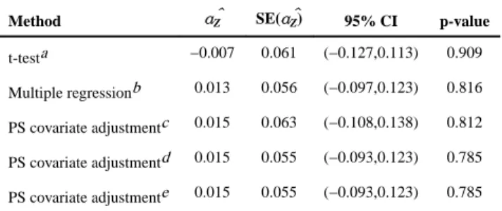
Results for five methods appear in Table 5. The first row of Table 5 presents the crude treatment effect estimate, i.e. −0.007, obtained without adjusting for any of the confounding covariates. This result indicates that the nerve block procedure can slightly relieve post-surgery pain compared to the traditional anesthesia procedure, though this conclusion is not statistically significant. However, after adjusting for the confounding factors, the PS covariate adjustment gives a positive treatment effect estimate of 0.015, suggesting that the nerve block procedure gives less pain relief. Again, this conclusion is not statistically significant. It is evident that both the analytic and empirical bootstrapping variance
estimators provide nearly identical standard errors (i.e. 0.055) for α̂Z and they are noticeably
smaller (by 14.5%) than the conventional standard error (i.e. 0.063) obtained directly from the covariate adjustment by PS without acknowledging the fact that the PS scores are estimated with errors. This result is consistent with what we observed in the simulation studies though the difference from the traditional variance estimator is not remarkably large. A potential interpretation is that the confounding effects are not large in this clinical
example. As a further comparison, we fit a multiple regression model including all the linear terms of the observed covariates in addition to the treatment allocation. The treatment effect estimate and its standard error are very close to the ones from the PS covariate adjustment with the proposed variance estimators, and the standard errors from the two methods are smaller than the one from the analysis without any covariate adjustment.
5. Discussion
In this paper, we show that the variance estimation of the treatment effect estimates, obtained directly from the PS covariate adjustment without acknowledging the fact that the PS scores are estimated with errors, is biased in general and could lead to invalid statistical
A
uthor Man
uscr
ipt
A
uthor Man
uscr
ipt
A
uthor Man
uscr
ipt
A
uthor Man
uscr
inferences. The availability of our user-friendly software would enable investigators to easily apply the proposed covariate adjustment by PS analysis scheme to their studies and make valid statistical inferences.
Treating the PS covariate adjustment as a two-stage analysis enables us to establish the asymptotic results of the treatment effect estimates and propose a valid analytic variance estimator. The closed form analytic variance estimator is accurate and asymptotically consistent. More importantly, as our simulations indicate, it is also robust to model miss-specifications where complex confounding structures exist. In addition to the analytic procedure, we also carry out an empirical bootstrap procedure that is straightforward but more computationally intensive. As shown in Simulation Studies section, the variance estimate from the proposed analytic variance estimators are not only very close to the true variance of treatment effect estimates but also they are smaller than that from the
conventional variance estimator where the PS uncertainty is ignored. One plausible explanation is that the correlation between the true (unknown) propensity scores and the treatment assignment is exaggerated by the correlation between the estimated propensity scores and the treatment assignment, leading to an inflated variance estimate. Similar pattern has been observed by Zou and Fine [14] where parameter estimates derived from the likelihood function with plug-in estimator of the nuisance parameter vector can be more efficient than the ones derived from the likelihood function with known nuisance parameter vector.
It should be noted that the treatment effect based on covariate adjustment by PS method is a conditional treatment effect estimate. For linear treatment effects, for example, continuous data where the treatment effect is obtained by comparing the mean difference, it is
collapsible, i.e. the conditional and marginal treatment effects are equivalent (e.g. [15]). The marginal and conditional treatment effects for binary outcomes are different if the treatment effect is evaluated through the odds ratio or risk ratio (e.g. [16]) since they are nonlinear treatment effects in these scenarios.
As an alternative to the covariate adjustment by PS, it is also common to run multiple regression analysis where all confounding factors are included as covariates in the regression model, in the same manner as we have done in Section 4. Our simulation results (not shown) indicate that the PS covariate adjustment analysis tends to provide as efficient treatment effect estimates as the multiple regression analysis when no complex confounding structures exist. However, the estimates from the PS covariate adjustment seem to be more robust than the ones from the multiple regression analysis when, for example, the linearity assumption is violated from the presence of complex confounding structures. This deserves further theoretical investigation, but is beyond the scope of this paper. Finally, it is worth mentioning that a limitation of all PS-based methods is that they can only adjust for observed confounding factors but not unobserved ones (e.g. [17]).
Acknowledgments
B. Zou and J. Shuster were partially supported by NIH grant 1UL1TR000064 from the National Center for Advancing Translational Sciences and H. Zhou was partially supported by NIH grants R01ES021900 and
A
uthor Man
uscr
ipt
A
uthor Man
uscr
ipt
A
uthor Man
uscr
ipt
A
uthor Man
uscr
P01CA142538. Authors would like to thank the editor and two anonymous reviewers for their constructive comments.
References
1. Johnston SC, Rootenberg JD, Katrak S, Smith WS, Elkins SJ. Effect of a US National Institutes of Health programme of clinical trials on public health and costs. Lancet. 2006; 367:1319–1327. [PubMed: 16631910]
2. Rosenbaum PR, Rubin DB. The central role of the propensity score observational studies for causal effects. Biometrika. 1983; 70:41–55.
3. Hade EM, Lu B. Bias associated with using the estimated propensity score as a regression covariate. Statistics in Medicine. 2014; 33:74–87. [PubMed: 23787715]
4. Mangano DT, Tudor LC, Dietzel C. The risk associated with aprotinin in cardiac surgery. The New England Journal of Medicine. 2006; 354(4):353–365. [PubMed: 16436767]
5. Stampf S, Graf E, Schmoor C. Estimators and confidence intervals for the marginal odds ratio using logistic regression and propensity score stratification. Statistics in Medicine. 2010; 29:760–769. [PubMed: 20213703]
6. An W. Bayesian propensity score estimators: incorporating uncertainties in propensity scores into causal inference. Sociological Methodology. 2010; 40:151–189.
7. Zigler CM, Watts K, Yeh RW, Wang Y, Coull BA, Dominici F. Model Feedback in Bayesian Propensity Score Estimation. Biometrics. 2013; 69:263–273. [PubMed: 23379793]
8. Murphy KM, Topel RH. Estimation and inference in two-step econometric models. Journal of Business and Economic Statistics. 1985; 3:370–379.
9. Efron B. Bootstrap methods: Another look at the jackknife. Annal of Statistics. 1979; 7:1–26. 10. Senn SJ. Covariate imbalance and random allocation in clinical trials. Statistics in Medicine. 1989;
8(4):467–475. [PubMed: 2727470]
11. Austin PC. An Introduction to Propensity Score Methods for Reducing the Effects of Confounding in Observational Studies. Multivariate Behav Res. 2011; 46(3):399–424. [PubMed: 21818162] 12. Rosenbaum PR. From Association to Causation in Observational Studies: The Role of Tests of
Strongly Ignorable Treatment Assignment. Journal of the American Statistical Association. 1984; 79(385):41–48.
13. Emura, T.; Wang, J.; Katsuyama, H. Technical Report of Mathematical Sciences. Chiba University; Japan: 2008. Assessing the Assumption of Strongly Ignorable Treatment Assignment Under Assumed Causal Models; p. 24
14. Zou F, Fine JP. A note on a partial empirical likelihood. Biometrika. 2002; 89(4):958–961. 15. Austin PC. The performance of different propensity score methods for estimating marginal hazard
ratios. Statistics in Medicine. 2013; 32:2837–2849. [PubMed: 23239115]
16. Senn S, Graf E, Caputo A. Stratification for the propensity score compared with linear regression techniques to assess the effect of treatment or exposure. Statistics in Medicine. 2007; 26:5529– 5544. [PubMed: 18058851]
17. Rubin DB. Estimating Causal Effects from Large Data Sets Using Propensity Scores. Annals of Internal Medicine, Part 2. 1997; 127:757–763.
Appendix I: Proof of Theorem 2.1
Let and denote the true parameter values of θ1 and θ2 under the models (2) and (4). The
MLEs of θ1 and θ2, i.e. θ̂1 and θ̂2 satisfy score equations:
(9)
A
uthor Man
uscr
ipt
A
uthor Man
uscr
ipt
A
uthor Man
uscr
ipt
A
uthor Man
uscr
(10)
Under standard regularity conditions, θ̂1 is consistent. Therefore, the maximization of the
quantity is asymptotically equivalent to the maximization of
. Thus, θ̂2 is consistent. Taking Taylor expansions on and at
, we obtain:
(11)
(12)
Plugging equations (11) and (12) into the score equations (9) and (10), we immediately obtain:
(13)
(14)
By the central limit theorem, we conclude the joint distribution of statistics:
is bivariate normal and given by the following:
A
uthor Man
uscr
ipt
A
uthor Man
uscr
ipt
A
uthor Man
uscr
ipt
A
uthor Man
uscr
where
, and .
By the law of large number theorem, the asymptotic equivalence of (13) can be written as the following:
(15)
Plugging (15) into (14) and applying the law of large number theorem, we have:
By the joint distribution of , we obtain the
asymptotic distribution of θ̂2:
(16)
where Σ = V2 + V2[CV1CT − RV1CT − CV1RT]V2 with
and hence the conclusions follow.
Appendix II: R Function for the Proposed Variance Estimators in PS
Covariate Adjustment
# dmat: data matrix
# 1) first column is outcome
# 2) second column is treatment assignment # 3) the rest are other observed covariates # boot.num: # of bootstrapping
# <=0 indicating two–stage # output:
# 1) trt.est: treatment effect estimate
# 2) trt.se: standard error based on the proposed estimator
# 3) naive.se: standard error based on conventional variance estimator twoStagePS = function(dmat, boot.num=0) {
n=dim(dmat)[1];
A
uthor Man
uscr
ipt
A
uthor Man
uscr
ipt
A
uthor Man
uscr
ipt
A
uthor Man
uscr
y=dmat[ ,1]; trt=dmat[ , 2];
x=as.matrix(dmat[,–c(1 ,2)]); psfit=glm(trt~x,family=binomial); ps=psfit$fitted;
yfit=lm(y~trt+ps);
ysum=(summary(yfit))$coefficients; if (boot.num <= 0) {
newx=cbind(rep(1,n), x); tps=trt–ps;
11th1=newx*matrix(tps,1,n)[,]; y.res=yfit$resid;
sigma2=sum(y.resˆ2)/(n–3); tem2=y.resˆ2/(2*sigma2) – 0.5;
12th2=cbind(y.res,trt*y.res,ps*y.res,tem2)/sigma2; alphaP=ysum[3,1];
ppstem1=ps*(1–ps)*y.res*alphaP/sigma2; ppstem2=trt*(1–ps)–(1–trt)*ps;
ppstem=ppstem1+ppstem2;
12th1=newx*matrix(ppstem,1,n)[,]; V1mat=t(11th1)%*%11th1;
V2mat=t(12th2)%*%12th2; Cmat=t(12th2)%*%12th1; Rmat=t(12th2)%*%11th1; new.V1=solve(V1mat); new.V2=solve(V2mat);
CVmat1=Cmat%*%new.V1%*%t(Cmat); CVmat2=Rmat%*%new.V1%*%t(Cmat); CVmat3=Cmat%*%new.V1%*%t(Rmat); CVmat=CVmat1–CVmat2–CVmat3;
Vmat=new.V2+new.V2%*%CVmat%*%new.V2; t.est=ysum[2,1];
t.se=sqrt(Vmat[2,2]); n.se=ysum[2,2];
return(list(trt.est=t.est,trt.se=t.se,naive.se=n.se)); }
boot.est=rep(0,boot.num); index=c(1:n);
for (i in 1:boot.num) {
nindex=sample(index,n,replace=T); ny=y[nindex];
ntrt=trt[nindex]; nx=x[nindex,];
npsfit=glm(ntrt~nx,family=binomial);
A
uthor Man
uscr
ipt
A
uthor Man
uscr
ipt
A
uthor Man
uscr
ipt
A
uthor Man
uscr
nps=npsfit$fitted; nyfit=lm(ny~ntrt+nps);
nysum=(summary(nyfit))$coefficients; boot.est[i]=nysum[2,1]
}
t.est=ysum[2,1];
t.se=sqrt(var(boot.est)); n.se=ysum[2,2];
return(list(trt.est=t.est,trt.se=t.se,naive.se=n.se)); }
A
uthor Man
uscr
ipt
A
uthor Man
uscr
ipt
A
uthor Man
uscr
ipt
A
uthor Man
uscr
A
uthor Man
uscr
ipt
A
uthor Man
uscr
ipt
A
uthor Man
uscr
ipt
A
uthor Man
uscr
ipt
T ab le 1Simulation Results with Simple Confounding Structures (T
rue ef fect size αZ =0.5) n (p , q ) A v erage α ̂Z
Monte Carlo SE(
α
̂)Z
Con v entional Modeling Analytic Modeling Bootstrapping A v erage
95% CI Co
v
erage
A
v
erage
95% CI Co
v
erage
A
v
erage
95% CI Co
v erage 500 (10, 0) 0.496 0.117 0.277 100.0 0.117 95.4 0.117 95.3 (10,10) 0.501 0.117 0.281 100.0 0.115 94.7 0.119 95.4 5000 (10, 0) 0.501 0.037 0.086 100.0 0.036 94.2 0.036 94.4 (10, 10) 0.500 0.038 0.086 100.0 0.036 94.1 0.036 94.3 n (p , q ) PS Stratif ication
IPW by PS
A
v
erage
α
̂Z
Monte Carlo SE(
α
̂)Z
A
v
erage
95% CI Co
v erage A v erage α ̂Z
Monte Carlo SE(
α
̂)Z
A
v
erage
95% CI Co
v erage 500 (10, 0) 0.534 0.107 0.161 99.5 0.501 0.145 0.132 93.3 (10,10) 0.531 0.110 0.163 99.3 0.504 0.151 0.132 91.9 5000 (10, 0) 0.533 0.033 0.050 97.4 0.499 0.046 0.044 94.5 (10, 10) 0.533 0.035 0.05 97.8 0.499 0.047 0.044 93.3 v
ariates and q=# of nuisance co
v
ariates; 5 strata were used for PS stratif
A
uthor Man
uscr
ipt
A
uthor Man
uscr
ipt
A
uthor Man
uscr
ipt
A
uthor Man
uscr
ipt
T
ab
le 2
Simulation Results with Simple Confounding Structures (T
rue ef
fect size
αZ
=1.00 and 1.50)
n
(p
,
q
)
A
v
erage
α
̂Z
Monte Carlo SE(
α
̂)Z
Con
v
entional Modeling
Analytic Modeling
Bootstrapping
95% CI Co
v
erage
95% CI Co
v
erage
A
v
erage
95% CI Co
v
erage
T
rue ef
fect size
αZ
=1.00
5000
(10, 0)
1.000
0.034
0.048
99.6
0.033
94.2
0.033
94.2
T
rue ef
fect size
αZ
=1.50
5000
(10, 0)
1.499
0.033
0.048
99.4
0.033
94.8
0.033
94.6
Note: n=sample size; p=# of confounding co
v
ariates and q=# of nuisance co
v
A
uthor Man
uscr
ipt
A
uthor Man
uscr
ipt
A
uthor Man
uscr
ipt
A
uthor Man
uscr
ipt
T ab le 3Simulation Results with Comple
x Confounding Structures (T
rue ef fect size αZ =0.5) n A v erage α ̂Z
Monte Carlo SE(
α
̂)Z
Con v entional Modeling Analytic Modeling Bootstrapping A v erage
95% CI Co
v
erage
A
v
erage
95% CI Co
v
erage
A
v
erage
95% CI Co
v
erage
Comple
x Confounding Structure I
a : treatment generated by (7) and response generated by (6)
500 0.497 0.120 0.283 100.0 0.125 94.7 0.118 93.6 5000 0.499 0.037 0.087 100.0 0.039 96.6 0.037 95.4 Comple
x Confounding Structure II
b: treatment generated by (5) and response generated by (8)
500 0.502 0.238 0.330 98.9 0.251 95.4 0.243 95.2 5000 0.503 0.077 0.100 98.9 0.079 95.4 0.077 95.2 See T
able 1 for the table le
gends
p
= 10 and
q
= 0
a Quadratic co
v
ariate term in the treatment assignment
b Quadratic co
v
A
uthor Man
uscr
ipt
A
uthor Man
uscr
ipt
A
uthor Man
uscr
ipt
A
uthor Man
uscr
ipt
T ab le 4 Baseline Distribution for Post-Sur
gery P ain Data Ner v e Block Anesthesia N Mean SE N Mean SE Age (year) 4806 57.06 15.81 1705 53.55 16.88 BMI 4806 29.00 6.98 1705 28.41 7.04 Sur
gery Duration (hour)
4806 3.87 2.08 1705 3.18 2.01 Ner v e Block Anesthesia N Pr oportion N Pr oportion Gender Male 2356 0.490 871 0.511 Female 2450 0.510 834 0.489
ICD9 Comorbidity Count
< 5
1194
0.248
411
0.241
5 ~ 9
1643
0.342
566
0.332
10 ~ 19
A
uthor Man
uscr
ipt
A
uthor Man
uscr
ipt
A
uthor Man
uscr
ipt
A
uthor Man
uscr
ipt
Table 5
Analysis Results for Post-Surgery Pain Data
Method α̂Z SE(α̂Z) 95% CI p-value
t-testa −0.007 0.061 (−0.127,0.113) 0.909
Multiple regressionb 0.013 0.056 (−0.097,0.123) 0.816
PS covariate adjustmentc 0.015 0.063 (−0.108,0.138) 0.812
PS covariate adjustmentd 0.015 0.055 (−0.093,0.123) 0.785
PS covariate adjustmente 0.015 0.055 (−0.093,0.123) 0.785
a
Two sample t-test without adjusting for any confounding factors
b
Multiple regression model including all observed covariates
c
d
with total 500 rounds of bootstrapping