Max-stable Processes for Threshold Exceedances
in Spatial Extremes
Soyoung Jeon
A dissertation submitted to the faculty of the University of North Carolina at Chapel Hill in partial fulfillment of the requirements for the degree of Doctor of Philosophy in the Department of Statistics and Operations Research.
Chapel Hill 2012
c O2012 Soyoung Jeon
ALL RIGHTS RESERVED
ABSTRACT
Max-stable Processes for Threshold Exceedances in Spatial Extremes (Under the direction of Richard L. Smith)
The analysis of spatial extremes requires the joint modeling of a spatial process at a large number of stations. Multivariate extreme value theory can be used to model the joint extremal behavior of environmental data such as precipitation, snow depths or daily temperatures. Max-stable processes are the natural generalization of extremal dependence structures to infinite dimensions arising from the extension of multivariate extreme value theory. However, there have been few works on the threshold approach of max-stable processes.
Acknowledgments
I wish to express my deepest gratitude to my faculty advisor, Dr. Richard L. Smith, for his support and guidance over the past five years. A great deal of my enthu-siasm for research stems from the opportunity to work with him. I have immense respect for him and deeply appreciate his inspiring suggestions, kind patience and trust throughout my graduate study.
I would also like to thank faculty members in Statistics Department for their help and guidance in the study of Statistics. I am also thankful for SAMSI of great opportunities working with research scientists in the field of spatial statistics, and especially I would like to thank to SAMSI working groups what I have been involved in, for very helpful comments and insights what I got.
A special thank you goes to my good fellow doctoral students. They provided me with lots of encouragement and empathy during the tough times of the research process. I am especially thankful to my dear friends for their sincere friendship and time sharing with me through the doctoral program.
Last but not least, I would like to express my loving gratitude to my parents and parents in law for their understanding and encouragement to follow my dreams. They instilled a drive in me that has helped me complete this five-year journey. I also would like to give special words to my husband and my sweet son. They always bring me a smile and make my life brilliant.
Table of Contents
List of Figures . . . . vii
List of Tables . . . . viii
1 Introduction . . . . 1
2 Background . . . . 3
2.1 Extreme Value Theory . . . 3
2.2 Dependence of Spatial Extremes: Extremal Coefficient . . . 6
2.3 Max-stable Processes . . . 8
2.3.1 Models of Max-stable Processes . . . 8
2.3.2 Fitting Max-stable Processes . . . 14
3 Threshold Approach of Max-stable Processes . . . . 18
3.1 Introduction to Threshold Approach . . . 18
3.2 Methodology for Exceedances over Threshold . . . 20
4 Asymptotic Behavior of Estimates for Dependence Parameters . . 24
4.1 Theoretical Framework of Threshold Approach . . . 24
4.1.1 Second-order Regular Variation Condition . . . 25
4.1.2 Spatial Structure and Sampling Design . . . 37
4.2 Asymptotic Properties: Asymptotic Normality and Consistency . . . . 42
5 Application . . . . 56
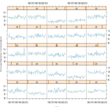
5.1 Max-stable Processes for Annual Maxima of Temperature . . . 57
5.2 Threshold Approach for Daily Temperature . . . 61
5.2.1 Modeling and Parameter Estimation . . . 62
5.2.2 Spatial Dependence of Thresholded Exceedances . . . 62
6 Discussion . . . . 67
6.1 Conclusion . . . 67
6.2 Future research . . . 68
Appendix . . . . 70
Bibliography. . . . 81
List of Figures
2.1 Realization of the Smith model . . . 11 2.2 Realization of the Schlather model . . . 12 3.1 Likelihood contribution according to four possible restrictions . . . 22
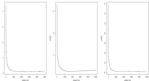
4.1 Graphical summary of asymptotic behavior for Smith model (i) . . . . 51 4.2 Extremal coefficient functions for the Smith model (i) . . . 51 4.3 Graphical summary of asymptotic behavior for Smith model (ii) . . . 53 4.4 Extremal coefficient functions for the Smith model (ii) . . . 53 4.5 Mean squared error of ˆα, ˆβ and ˆγ for Smith (i) from left to right . . . 55 4.6 Mean squared error of ˆα, ˆβ and ˆγ for Smith (ii) from left to right . . . 55
List of Tables
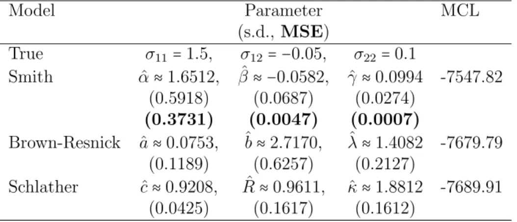
5.1 Fitting max-stable processes for annual maxima of temperature . . . . 58
5.2 Composite MLE’s for Z generated from Smith model . . . 60
5.3 Composite MLE’s for Ẑ generated from Smith model . . . 60
5.4 Composite MLE’s for Z generated from Schlather model . . . 61
5.5 Composite MLE’s for Ẑ generated from Schlather model . . . 61
5.6 Fitting max-stable processes for exceedances of daily temperature . . 63
5.7 Summary of the marginal analysis with u=.62738 . . . . 63
5.8 Pairs of site with short distance and independence . . . 66
5.9 Pairs of site with long distance and dependence . . . 66
Chapter 1
Introduction
Extreme value theory and its application are dealing with related methodologies to understand phenomena of rare events such as flooding, high temperatures and precip-itations in environmental data. It is well known and widely publicized that extreme temperatures are relevant to the problem of sudden deaths from heatwaves and also, extreme levels of air pollution have strong influence on human health outcomes. Ex-treme environmental data involve in these statistical issues that have arisen in the study of human health and the application of extreme value analysis can be used to analyze the problems.
surface. Therefore one ultimately requires the modeling of spatial extremes, and a spatial dependence among the different locations is of interest. Cooley et al. [2012] introduces several references which dealt with issues of spatial extremes.
It is natural to consider a stochastic process when the sample maxima are ob-served at each site of a spatial process. Max-stable processes have been developed as a class of stochastic processes suitable for studying spatial extremes. The first general characterization of max-stable processes was by de Haan [1984], and Smith [1990] has constructed a special case of max-stable processes which provides the useful interpretation of extreme rainfall models. Statistical techniques based on the Smith’s max-stable model have been developed by Coles [1993] and Coles and Tawn [1996] and the well-known classes of max-stable processes are discussed further by Schlather [2002] and Kabluchko, Schlather and de Haan [2009].
Due to the complexity and unavailability of the full likelihood for the max-stable model, Padoan, Ribatet and Sisson [2010] developed the maximum composite like-lihood approach to fit max-stable processes. However, the research on max-stable processes with exceedances over threshold has hardly been considered.
In this thesis, we are concerned with the development of a threshold approach us-ing max-stable processes in spatial extremes. We review the background of extreme value theory, max-stable processes and spatial dependence measure in Chapter 2. In Chapter 3 we introduce our methodology to model exceedances over threshold using max-stable processes. Chapter 4 develops a theoretical framework and asymptotic properties, which are illustrated with a simulation study. In Chapter 5 the proposed approach is applied to the analysis of temperatures in North Carolina, and the con-clusion and discussion are drawn in Chapter 6.
Chapter 2
Background
2.1
Extreme Value Theory
In this section, we outline the background of univariate extreme sequences of indepen-dent and iindepen-dentically distributed (i.i.d.) random variables. Univariate extreme value theory can be extended to multivariate extremes. Fundamental theory and practice of univariate and multivariate extremes have been well-established.
LetX1,⋯, Xn be i.i.d. random variables with the same probability distributionF and let Mn=max(X1,⋯, Xn) be the maximum. IfMn converges under renormaliza-tion to some nondegenerate limit, then the limit must be a member of the parametric family, i.e. there exist suitable normalizing constants an>0, bn and the distribution
̃
G such that
P{Mn−bn an
≤x}=Fn(anx+bn)Ð→G̃(x), asn→∞ (2.1)
whereG̃is a nondegenerate distribution function. The distribution functionsG̃which are possible limit laws for maxima of i.i.d. sequences form the class of so-called
max-stable distributions. It is said that a nondegenerate functionG̃is max-stable if, there
called three Extreme Value Distributions (EVD).
Type I (Gumbel): G̃(x) = exp(−e−x), −∞<x<∞; Type II (Fr´echet): G̃(x) = ⎧⎪⎪⎪⎪⎨
⎪⎪⎪⎪ ⎩
0, x≤0,
exp(−x−α), x>0, α>0; Type III (Weibull): G̃(x) = ⎧⎪⎪⎪⎪⎨
⎪⎪⎪⎪ ⎩
exp(−(−x)α), x≤0, α>0,
1, x>0.
The Three Types Theorem was originally stated by Fisher and Tippett [1928] and
derived rigorously by Gnedenko [1943]. Leadbetter, Lindgren and Rootz´en [1983] showed that a distribution function is max-stable if and only if it is of the same type as one of the three extreme value distributions listed.
The three types of EVD can be represented as G combining into a single para-metric family distribution, which is called the Generalized Extreme Value (GEV) distribution:
G(x;µ, ψ, ξ)=exp{−(1+ξx−µ σ )
−1/ξ
+
},
where y+ = max(0, y), µ is a location parameter, σ > 0 is a scale parameter and ξ is a shape parameter which determines the tail behavior. The Generalized Extreme Value distributionG has a max-stable property: if X1,⋯, XN are i.i.d. fromG, then max(X1,⋯, XN) also has the same distribution, i.e.
GN(x)=G(ANx+BN) for existing constantsAN >0, BN.
The form of the limiting distribution is invariant under monotonic transformation. Therefore, without loss of generality we can transform the GEV distribution into a
specific form and consider the Fr´echet form for convenience:
P{X≤x}=exp(−x−α), x>0
where α >0. The case α =1 is called unit Fr´echet. For our current application, we use the GEV distribution transformed into the unit Fr´echet distribution,
P⎧⎪⎪⎨⎪⎪
⎩(
1+ξMn−µ σ )
1/ξ
+
≤z⎫⎪⎪⎬⎪⎪
⎭=
P(Z ≤z)=exp(−1/z), z >0,
and note that the unit Fr´echet form is a distribution which has the max-stable prop-erty.
Multivariate extreme value theory is concerned with the joint distribution of ex-tremes of two or more random variables. Suppose we have i.i.d. observations from a K-dimensional random vector(Xi1,⋯, XiK), i=1,2,⋯, and letMn=(Mn1,⋯, MnK) denote theK-dimensional vector of componentwise maxima,Mnk =max(X1k,⋯, Xnk), k=1,⋯, K. A limit distribution for Mn is said to exist if there exist ank >0 and bnk for k=1,⋯, K such that
lim n→∞P{
Mn1−bn1 an1
≤x1,⋯,
MnK −bnK anK
≤xK}=G(x1,⋯, xK). (2.2)
Then G is a multivariate extreme value distribution and if (2.2) holds, then G is max-stable if there exist AN k>0 and BN k, k =1,⋯, K, for any N >1 such that
GN(x1,⋯, xK)=G(AN1x1+BN1,⋯, AN KxK+BN K).
If G is a multivariate EVD, the marginal distribution must be represented by the GEV distribution and each marginal GEV distribution can be transformed into unit Fr´echet margin, which has the max-stable property.
to an infinite-dimensional generalization with spatial processes. The infinite-dimensional extremes has quite analogous extension to the theory of max-stable random vector. Let S be a study region and denote s as a location in the study region. If there exist normalizing sequences an(s) and bn(s) for all s ∈ S such that the sequence of stochastic processes
max i=1,⋯,n
Xi(s)−bn(s) an(s)
D
Ð→Y(s) (2.3)
where Y(s) is non-degenerate for all s, then the limit process Y(s) is a max-stable process. A finite sample {Y(s1),⋯, Y(sD)} can be concerned as a realization of a spatial process Y(s) for more realistic setting.
2.2
Dependence of Spatial Extremes: Extremal Coefficient
In the analysis of spatial extremes, one can be interested with measuring spatial dependence among locations. Quantifying spatial dependence has been studied in the field of geostatistics and one of metrics is the variogram which is typically used in the geostatistics. Let Y(s) be a stationary stochastic process and suppose
Var[Y(s)−Y(s′)]=2γ(s−s′) for all s, s′∈S.
The quantity 2γ(⋅), so-called variogram, depends on the increments s−s′ and γ(⋅) has been called semivariogram which determines the degree of spatial dependence of Y(⋅) (see Matheron [1987] and Cressie [1993]). However the (semi-)variogram is an inadequate tool to analyze spatial dependence of extreme data, since the traditional geostatistics does not deal with the tail distribution.
In this section, we focus on another metric, extremal coefficient, to characterize the tail dependence. Suppose a d-dimensional random variable X has the common marginal distributionsF(x). The extremal coefficientθdcan be defined by the relation
P r{max(X1,⋯, Xd)≤x}=Fθd(x).
Assuming the standard form of unit Fr´echet distribution on each margin, we can characterize the dependence among the components of marginal distribution inde-pendently. Let Z be d-dimensional maxima with unit Fr´echet margins and whose multivariate extreme value distribution is expressed as
P r{Z1≤z1,⋯, Zd≤zd}=exp{−V(z1,⋯, zd)}, (2.4)
where the exponent measure V is a homogeneous function of order −1. Due to the homogeneity ofV, the extremal dependence can be measured byV which implies
complete dependence ifV(z1,⋯, zd)=max(z11,⋯,z1d), complete independence if V(z1,⋯, zd)=z11 + ⋯ +z1d.
The relationship between the extremal coefficient θd and the exponent measure V is drawn from
P r{Z1≤z,⋯, Zd≤z}=exp(−θd
z ), (2.5)
θd=V(1,⋯,1)
where 1≤θd≤d with the lower and upper bounds corresponding to complete depen-dence and complete independepen-dence, respectively.
We consider a pairwise extremal coefficient as a special case of (2.5) in the spatial domain. LetY(s)be a spatial process with unit Fr´echet margin for alls∈S and then extremal dependence between different sites s and s′ is obtained by,
P r{Y(s)≤y, Y(s′)≤y}=exp(−θ(s−s
′)
A naive estimator of the pairwise extremal coefficient is proposed by Smith [1990];
̂
θ(s−s′)= n ∑n
i=1min{Yi(s)−1, Yi(s′)−1} .
Schlather and Tawn [2003] investigated theoretical properties of the extremal coef-ficients and proposed self-consistent estimators of θ (i.e. estimators that satisfy the properties of extremal coefficients) for the multivariate and spatial case.
2.3
Max-stable Processes
2.3.1
Models of Max-stable Processes
Now consider the max-stable processes as an infinite dimensional generalization of extreme value theory. SupposeX(s), s∈S is a stochastic process, where S ⊆Rdis an arbitrary index set. We can interpret X(⋅) as a spatial process with an appropriate generalization of (2.2) as following: for each n ≥1, there exist continuous functions an(s)positive and bn(s)real, for s∈S such that
P rn{X(sj)−bn(sj) an(sj)
≤x(sj), j=1,⋯, K}Ð→Gs1,⋯,sK(x(s1),⋯, x(sK)). (2.6)
Then Gs1,⋯,sK is a multivariate extreme value distribution and the limiting process
is max-stable if (2.6) holds for all possible subsets s1,⋯, sK ∈ S. Note that this is
equivalent to the expression in equation (2.3).
We are interested in modeling and estimation using max-stable processes for ex-tremes observed at each site of a spatial process. A general representation of max-stable processes was first given by de Haan [1984]. The conceptual idea of max-max-stable processes can be constructed by two components: a stochastic process {W(s)}and a Poisson process Π with intensitydζ/ζ2 on(0,∞). If{W
i(s)}i∈Nis independent copies of W(s)withE[W(s)]=1 for all sand ζi∈Π, i≥1,is points of the Poisson process,
then
Y(s)=max
i≥1 ζiWi(s), s∈S
is a max-stable process with unit Fr´echet margins. The joint distribution function for max-stable processes is given as
P(Y(s)≤y(s), s∈S)=exp(−E[sup s∈S {
W(s)
y(s) }]), (2.7) or practically, it can be rewritten to the equivalent equation (2.4) on the set{s1,⋯, sD}⊂ S, where
V(y1,⋯, yD)=E[ sup d=1,⋯,D{
W(sd)
y(sd) }]. (2.8)
The construction of different max-stable processes can be differentiated from different choices of the W(s) process and the well-known classes of max-stable processes are discussed by Smith [1990], Schlather [2002] and Kabluchko, Schlather and de Haan [2009].
The Smith Model
Smith [1990] proposed new max-stable stochastic processes under the following con-struction. Let {(ζi, si), i≥ 1} denote the points of a Poisson process on (0,∞)×Rd with intensity measure ζ−2dζds. Define a non-negative function {f(x)} on Rd such that ∫ f(x)dx=1 and
Y(s)=max
i≥1 ζif(s−si).
Smith considered a specific setting, so-called a Gaussian extreme value process, where f(x) = (2π)−d∣Σ∣−1/2exp(− 1
2x
TΣ−1x) is a multivariate normal density with covariance matrix Σ. Then the joint distribution at two sites is obtained in a closed form,
P(Y(s1)≤y1, Y(s2)≤y2) =exp⎧⎪⎪⎨⎪⎪
⎩−
1 y1
Φ⎛
⎝
a 2+
1 alog
y2 y1
⎞ ⎠−
1 y2
Φ⎛
⎝
a 2 +
1 alog
y1 y2
⎞ ⎠ ⎫⎪⎪ ⎬⎪⎪ ⎭
(2.9)
where a = √(s1−s2)TΣ−1(s1−s2) and Φ is the standard normal cumulative distri-bution function. The positive valuea represents the spatial dependence according to the distance between two sites. The limits a→0 and a→∞ correspond to complete dependence and independence, respectively. One may write out the pairwise extremal coefficients explicitly as
θ(h)=2Φ⎛
⎝ √
(s1−s2)TΣ−1(s1−s2) 2
⎞ ⎠
where h is the Euclidean distance, ∥s1−s2∥, between two stations. Realizations of the Gaussian extreme value process are shown in Figure 2.1.
The Schlather Model
More recently, Schlather [2002] suggested a new class of max-stable processes based on a stationary random field with finite expectation. Let Wi(s), i =1,2,⋯ be i.i.d. stochastic processes on Rd, and let µ=E[max(0, W
i(s))]<∞and {ζi, i≥1} denote the points of a Poisson process on (0,∞) with intensity measure µ−1ζ−2dζ. Then a stationary max-stable process with unit Fr´echet margins can be obtained by:
Y(s)=max
i≥1 ζimax(0, Wi(s))
0.5 1.0 1.5 2.0 2.5 3.0
0 2 4 6 8 10 12 14 0 2 4 6 8 10 12 14
(a)σ11=σ22=9/8 andσ12=0
1 2 3 4 5
0 2 4 6 8 10 12 14 0 2 4 6 8 10 12 14
(b)σ11=σ22=9/8 andσ12=1
Figure 2.1: Realization of the Smith model with different covariance matrices from SpatialExtremes R package
where the Wi are i.i.d. copies of W(s) for all i. The max-stable process provides a more flexible class of max-stable processes by taking a stationary random process Wi(s) and it also gives the interpretation of spatial storm modeling. The spatial rainfall events are explained by the structure of spatial dependence but this process represents more general case than Smith’s model. The shape of storms is deterministic withf(⋅)in Smith’s model while the storms may have a random shape in Schlather’s model.
Schlather specified a model for a stationary Gaussian random process. LetWi be a stationary Gaussian random field with unit variance, correlationρ(⋅)and µ−1 =√2π, then the process Y(s) is called as an extremal Gaussian process and the bivariate marginal distributions are given explicitly by
P(Y(s1)≤y1, Y(s2)≤y2) =exp⎧⎪⎪⎨⎪⎪
⎩− 1 2 ⎛ ⎝ 1 y1 + 1 y2 ⎞ ⎠ ⎛ ⎝1+
√
1−2(ρ(h)+1) y1y2
(y1+y2)2
(a) sill=range=smooth=1 (b) sill=smooth=1 and range=1.5
Figure 2.2: Realization of the Schlather model with different correlation functions from SpatialExtremes R package; (a) Whittle-Mat´ern correlation and (b) Powered exponential correlation
where h is the Euclidean distance between station s1 and s2. The pairwise extremal coefficient is obtained by
θ(h)=1+(1−ρ(h)
2 )
1/2 .
Figure 2.2 shows the realizations of the extremal Gaussian process with different correlation functions.
The Schlather model cannot attain the case of independence for extremes as the distance h increases, since the extremal coefficient θ(h) is in the interval [1,1.838]. To overcome the problem, the processWi(s)can be restricted to a random setB, i.e.,
Y(s)=max
i ζiWi(s)IBi(s−Si)
whereIB is the indicator function of a compact random setB⊂S andSiare the points of a Poisson process. If Wi is a Gaussian process, the bivariate marginal distribution
is
P(Y(s1)≤y1, Y(s2)≤y2) =exp⎧⎪⎪⎨⎪⎪
⎩−(
1 y1 +
1 y2)
⎡⎢ ⎢⎢ ⎢⎣1−
α(h) 2
⎛ ⎝1−
√
1−2(ρ(h)+1) y1y2
(y1+y2)2
⎞ ⎠ ⎤⎥ ⎥⎥ ⎥⎦ ⎫⎪⎪ ⎬⎪⎪ ⎭
where α(h) = E{∣B ∩(h+B)∣}/E(∣B∣) ∈ [0,1]. One possible choice for the set B is a disc of radius r and it leads to take α(h) ≐ {1−∣h∣/(2r)}+, which equals to 0 representing the independence of extremes in the case of ∣h∣ > 2r (see details in Davison and Gholamrezaee [2012]). The extremal coefficient is
θ(h)=2−α(h){1−(1−ρ(h)
2 )
1/2
},
which accounts independent extremes by taking any value in the interval[1,2].
The Brown-Resnick Process
The original Brown-Resnick process was introduced with the Brownian motion for max-stable process by Brown and Resnick [1977]. Kabluchko, Schlather and de Haan [2009] has constructed a more general class of max-stable processes, so-called the
Brown-Resnick process, by replacing the Brownian motion by other stochastic
pro-cesses.
the bivariate distributions for the Brown-Resnick process associated to the variogram γ is given by
P(Y(s1)≤y1, Y(s2)≤y2) =exp⎧⎪⎪⎨⎪⎪
⎩− 1 y1 Φ⎛ ⎝ √
γ(h)
2 +
1
√
γ(h)log y2 y1 ⎞ ⎠− 1 y2 Φ⎛ ⎝ √
γ(h)
2 +
1
√
γ(h)log y1 y2 ⎞ ⎠ ⎫⎪⎪ ⎬⎪⎪ ⎭ (2.11)
where Φ is the standard normal distribution function andhis the Euclidean distance between location s1 and s2. The pairwise extremal coefficients are given as
θ(h)=2Φ⎛
⎝ √
γ(h) 2
⎞ ⎠.
2.3.2
Fitting Max-stable Processes
We are interested with the analysis of spatial extremes at a large number of stations and the standard methods of estimation, such as MLE and Bayes methods, require a full likelihood. However the full likelihood for the max-stable processes may not be available analytically, because there are difficulties to achieve the expression of differentiation for the joint distribution function (2.7) and to calculate the exponent measure (2.8) due to the complexity of its analytic form. With the lack of an explicit form of the joint distribution, Padoan, Ribatet and Sisson [2010] developed a pair-wise composite likelihood approach to fit max-stable processes, based on a composite likelihood method by Lindsay [1988].
For a parametric statistical model with density function family {f(y;ψ)∶y∈Y⊆
RK, ψ ∈Ψ ⊆Rd} and a set of marginal or conditional events {I
k ∶k ∈ K} subset of some sigma algebra on Y, the composite log-likelihood is defined by
lC(ψ;y)= ∑
k∈K
wklogf(y∈Ik;ψ),
where logf(y∈Ik;ψ) is the log-likelihood associated with event Ik and {wk}k∈K are
nonnegative weights.
A composite score function DψlC(ψ;y)is defined by first-order partial derivatives of lC(ψ;y) with respect to ψ and then the maximum composite likelihood estimator of ψ, if it is unique, is obtained by solving DψlC( ̂ψM CLE;y)= 0. Second-order par-tial derivatives of the composite score function yield the Hessian matrix HψlC(ψ;y). Under appropriate conditions based on Lindsay [1988] and Cox and Reid [2004], the maximum composite likelihood estimator may have consistency and asymptotically normality as
̂
ψM CLE ∼N(ψ,I˜(ψ)−1) with ˜I(ψ)=H(ψ)J(ψ)−1H(ψ),
where H(ψ)=E{−HψlC(ψ;Y)} is the expected second order derivatives of the score function, and the covariance matrix of the score function is J(ψ)=V{DψlC(ψ;Y)}, which are analogues of the expected information matrix and the variance of the score vector. The maximum composite likelihood estimator may not be asymptotically efficient in that ˜I(ψ)−1, the inverse of the Godambe information matrix, may not attain the Cram´er-Rao bound although it can be unbiased.
Pairwise Composite Likelihoods in Spatial Extremes
AssumeM i.i.d. replications of a stochastic process with bivariate densitiesf(yi, yj;ψ), 1≤i, j ≤K, in a spatial region with K locations. Then the pairwise composite log-likelihood is defined by
lP(ψ;Y)=
M ∑ m=1
K−1 ∑ i=1
K ∑ j=i+1
wijlogf(ymi, ymj;ψ), (2.12)
where(i, j)is a pair of stations andwij is nonnegative weight functions. One may set the weight as an indicator function, i.e.,wij =1 if∥s1−s2∥≤δ, and 0 otherwise. The
maximum pairwise composite likelihood estimator (MCLE), ˆψ, is chosen to maximize
Padoan, Ribatet and Sisson [2010] stated the asymptotic properties of MCLE based on the joint estimation, which maximizes the pairwise composite likelihood instead of the full likelihood. For the estimation, a pairwise composite log-likelihood is constructed as the form (2.12) and we consider the bijection (Yi, Yj) =g(Zi, Zj), where g is some monotonic increasing transformation to the unit Fr´echet. Then by change of variables, we represent the bivariate density over GEV margins as the form,
fYi,Yj(yi, yj)=fZi,Zj[g−
1(yi, yj)]∣J(yi, yj)∣,
where fZi,Zj(zi, zj) denotes the joint density of max-stable processes and the
deter-minant of the Jacobian is given by
∣J(yi, yj)∣= 1 σiσj
(1+ξi(yi−µi) σi
)
1/ξi−1
+
(1+ξj(yj −µj) σj
)
1/ξj−1
+
.
GEV marginal parameters and the dependence parameters can be estimated in a uni-fied framework by the change of variable technique. Variances of parameter estimates are provided through the inverse of the Godambe information matrix, with estimates of the matrices H(ψ) and J(ψ) given by
ˆ
H(ψˆM CLE)=− M ∑ m=1
K−1 ∑ i=1
K ∑ j=i+1
Hψlogf(ymi, ymj; ˆψM CLE)
and
ˆ
J(ψˆM CLE)= M ∑ m=1
{K∑−1 i=1
K ∑ j=i+1
Dψlogf(ymi, ymj; ˆψM CLE)}×
{K∑−1 i=1
K ∑ j=i+1
Dψlogf(ymi, ymj; ˆψM CLE)} T
.
In practice, the matrix ˆH is obtained through the numerical maximization routine and the explicit form of ˆJ is also derived [Padoan, Ribatet and Sisson, 2010, Appendix A.5].
Chapter 3
Threshold Approach of Max-stable
Processes
3.1
Introduction to Threshold Approach
Consider the distribution of all observations X over a high threshold u and let Y = X−u>0, then
Fu(y)=P r{Y ≤y∣Y >0}=
F(u+y)−F(u) 1−F(u) .
As u → x0 = sup{x ∶ F(x) < 1}, we can find a limit H called Generalized Pareto
Distribution (GPD)
Fu(y)≈H(y;σu, ξ)=1−(1+ξ y σu)
−1/ξ
+
. (3.1)
Pickands [1975] established the rigorous connection between the classical extreme value theory and the generalized Pareto distribution and proved that the limit of the form (3.1) exists if and only if there exist normalizing constants and the limiting form of H such that the classical extreme value limit (2.1) holds. Thus the limit result for exceedances over thresholds is equivalent to the limit distribution for maxima in this sense.
As an another statistical approach for threshold exceedances, the Point Process Approach is introduced by Smith [1989]. This approach considers a process based on a two dimensional plot of exceedance times and exceedance values, which has been developed from the point process viewpoints of extreme values by Leadbetter, Lindgren and Rootz´en [1983].
Under the proper normalization, the asymptotic theory of threshold exceedances proved that the process behaves like a nonhomogeneous Poisson process. A nonho-mogeneous Poisson process on a domain D is denoted by an intensity λ(x), x ∈ D, such that if A is a measurable subset of D and N(A) is the number of points in A, then N(A) has a Poisson distribution with mean
Λ(A)=∫ A
λ(x)dx.
For the present application, we denote(Ti, Yi)as the time of theith exceedance of the threshold and the observed excess valueYi>u, then the probability of observing an exceedance in an infinitesimal region t<Ti <t+dt, y<Yi <y+dy can be written as
1 σ(1+ξ
y−µ σ )
−1/ξ−1
+
dydt, y>µ. (3.2)
of T units, then the likelihood associated with the events (Ti, Yi),1≤i≤N, is N
∏ i=1
λ(Ti, Yi)⋅exp{−∫
Dλ(t, y)dtdy}
=∏N i=1
{1
σ(1+ξ Yi−µ
σ )
−1/ξ−1
+
}⋅exp{−T(1+ξu−µ σ )
−1/ξ
} (3.3)
and (3.3) is maximized with respect to unknown parameters (µ, σ, ξ).
For the inhomogeneous case the parameters µ, σ and ξ are all allowed to be time-dependent, denoted byµt, σt and ξt. Thus (3.2) is extended by the form
1 σt
(1+ξt y−µt
σt
)
−1/ξt−1
+
dydt, y>µt.
and if we also allow the threshold ut to depend on time t, the likelihood associated with (3.3) is now
∏ i
{ 1
σTi
(1+ξTi
Yi−µTi
σTi
)
−1/ξTi−1
+
}⋅exp{−∫ T
0 ( 1+ξt
ut−µt σt
)
−1/ξt
dt}.
3.2
Methodology for Exceedances over Threshold
As in the univariate case, the threshold method has been developed in the multivariate case as well. Let(x0, y0)denote the upper endpoint ofF, where(x0, y0)=sup{(x, y)∶ F(x, y)<1}, and define the conditional distribution of (X−u, Y −v) givenX >uor Y >v,
Fu,v(x, y)= F(u+x, v+y)−F(u, v)
1−F(u, v) . (3.4)
Then the conditional distribution of bivariate exceedances converges to H where H is a multivariate generalized Pareto distribution by Rootz´en and Tajvidi [2006].
In this dissertation we develop an alternative methodology for threshold exceedances using max-stable processes with unit Frech´et margins. We suggest the modeling of the bivariate threshold exceedances by assuming that the asymptotic distribution
holds exactly above a threshold and it leads to a simplified dependence structure for max-stable processes as we characterize the dependence among the components of bivariate marginal distribution in (2.9), (2.10) and (2.11).
The likelihood representation for this threshold method is also developed to fit the model and this has a similar idea by Smith, Tawn and Coles [1997] which establishes a joint distribution for Markov chains where the bivariate distributions were assumed to be of bivariate extreme value distribution form above a threshold.
Suppose we have annual maxima {Yt∗s, t∗=1,⋯, T∗, s=1,⋯, D} whereYt∗s is the value at site s in yeart∗. We assume the vectors {Yt∗s}are independent for different t∗ with joint densities given by a max-stable process, i.e., an explicit expression for its bivariate joint distribution is known and the marginal distributions are unit Fr´echet for each t∗ and s. Then the joint bivariate distribution of the annual maxima, FAM is written by
FAM(yt∗s, yt∗s′;θ)=P r{Yt∗s≤yt∗s, Yt∗s′ ≤yt∗s′;θ},
whereθis the dependence parameter which can be estimated by the max-stable model. Now suppose that the daily data are {Xts, t = 1,⋯, T, s = 1,⋯, D} and the joint bivariate distribution function is FDA(xts, xts′;θ). Assume that the daily data Xts form i.i.d. random processes and the annual maxima areYt∗s. Then the relationship between their bivariate distributions is
FDA(xts, xts′;θ)=P r{Xts≤xts, Xts′ ≤xts′;θ}
=FAM(xts, xts′;θ)1/M (3.5)
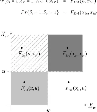
convenience. Then we observe exceedances {Xts}such that Xts >u. Let δs=I(Xts> u) where I is the indicator function. We can obtain the following joint distribution of (δs, Xts, δs′, Xts′) from four possible regions by including or excluding the interval over threshold u (see Figure 3.1),
P r{δs=0, δs′ =0} = FDA(u, u) P r{δs=1, δs′ =0, Xts<xts} = FDA(xts, u) P r{δs=0, δs′ =1, Xts′ <xts′} = FDA(u, xts′)
P r{δs=1, δs′ =1} = FDA(xts, xts′).
Figure 3.1: Likelihood contribution according to four possible restrictions
We extend the threshold version of max-stable processes and apply the maximum composite likelihood method on it. The likelihood contribution of the pair (xts, xts′) derived from the joint bivariate density can be obtained by
L(Xts, Xts′;θ,η)=
⎧⎪⎪⎪ ⎪⎪⎪⎪⎪ ⎪⎪⎪⎪ ⎨⎪⎪ ⎪⎪⎪⎪⎪ ⎪⎪⎪⎪⎪ ⎩
FDA(u, u) if xts≤u, xts′ ≤u, ∂
∂xtsFDA(xts, u) if xts>u, xts′ ≤u,
∂
∂xts′FDA(u, xts′) if xts≤u, xts′ >u, ∂2
∂xts∂xts′FDA(xts, xts′) if xts>u, xts′ >u.
where θ is the dependence parameter vector and η is a vector of marginal GEV parameter. Combining the above likelihood representation with a pairwise likelihood, we assume T i.i.d. replications of a stochastic process with bivariate densities of the unit Frech´et margins L(Xts, Xts′;θ,η),1 ≤ s, s′ ≤ D. Then the pairwise composite log-likelihood for a thresholded process is
l(θ,η)=
T ∑ t=1
D−1 ∑ s=1
D ∑ s′=s+1
wss′logL(Xts, Xts′;θ,η)= T ∑ t=1
lt(θ,η) (3.6)
where lt(θ,η) = ∑s=1D−1∑Ds′=s+1wss′logL(Xts, Xts′;θ,η0), (s, s′) is a pair of different stations and T is a number of observations. In practice, the marginal parameter η
will be estimated but we letηbe the true valueη0 to simplify theoretical justification. Thus we fix the marginal GEV parameters η = η0 and estimate the dependence parameterθ. A dependence parameterθcan be estimated by maximizing the pairwise composite likelihood function (3.6) with the known valueη0.
Suppose X(t) =(X
ts, Xts′) and denote the composite score functions by pairwise log-likelihood derivatives as
D(θ;X(t))= ∂lt(θ,η0)
∂θ ,
D(θ;X(1),⋯,X(T))=Dθ0l(θ,η0;X
(1),⋯,X(T))=∑T t=1
D(θ;X(t)).
Then the estimating equations
D(̂θ;X(1),⋯,X(T))=Dθl(̂θ,η0;X(1),⋯,X(T))=0.
Chapter 4
Asymptotic Behavior of Estimates
for Dependence Parameters
4.1
Theoretical Framework of Threshold Approach
Suppose that (Xi, Yi), i = 1,⋯, n, is a sequence of i.i.d. random vectors and F be the common distribution of (Xi, Yi) with marginal distributions F1 and F2. A distribution function F is said to be in the domain of attraction of a distribution function G, shortlyF ∈D(G), if
lim n→∞F
n(a
nx+bn, cny+dn)=G(x, y), an, cn>0 and bn, dn∈R (4.1) for all x and y. The two marginals of G(x,∞) and G(∞, y) are one-dimensional extreme value distributions satisfying
lim n→∞F
n
1(anx+bn) = exp{−(1+ξ1x)−1/ξ1}, lim
n→∞F n
2(cny+dn) = exp{−(1+ξ2y)−1/ξ2} where ξ1 and ξ2 are real parameters.
taking logarithms can be expressed as
lim
t→∞t{1−F(atx+bt, cty+dt)}=−logG(x, y)=∶Φ(x, y) (4.2) and it is checked easily that (4.2) implies that
lim
t→∞Fbt,dt(atx, cty)=tlim→∞(1−
t{1−F(atx+bt, cty+dt)} t{1−F(bt, dt)} ) =1−−logG(x, y)
−logG(0,0) =∶H(x, y)
where H is a bivariate generalized Pareto distribution. It has been illustrated that H is a good approximation of Fbt,dt in the sense that
lim
t→∞0<(a sup
tx,cty)<(x0−bt,y0−dt)
∣Fbt,dt(atx, cty)−H(x, y)∣=0,
if and only ifF is in the maximum domain of attraction of the corresponding extreme value distribution G (Rootz´en and Tajvidi [2006]).
4.1.1
Second-order Regular Variation Condition
Definition 1. A function f(x) is regular varying with index τ1 if for some τ1∈R,
lim t→∞
f(tx) f(t) =x
τ1, x>0.
The function f(x) is second-order regular varying with the first order τ1 and the
second order τ2 if there exists a function q(t)→0 as t→∞such that
lim t→∞
f(tx) f(t) −xτ1
q(t) =x
τ2, x>0.
Just as in the univariate case, the representation of bivariate regular variation exists: the function f(x, y)∶R2
+→R+ is regular varying of index τ if
lim t→∞
f(tx, ty)
f(t, t) =r(x, y)
where r(λx, λy)=λτr(x, y)for some λ>0. See Resnick [2007] for the related discus-sion of multivariate regular variation.
Suppose that the following second-order regular variation condition holds (de Haan and Ferreira [2006]): there exists a positive or negative functionαwith limt→∞α(t)=0 and a function Qnot a multiple of Φ such that
lim t→∞
t{1−F(atx+bt, cty+dt)}−Φ(x, y)
α(t) =Q(x, y) (4.3)
locally uniformly for (x, y) ∈ (0,∞]×(0,∞]. Define Ui as the inverse function of 1/(1−Fi), i=1,2 and it is known that for x, y>0,
lim t′→∞
U1(t′x)−U1(t′) a(t′) =
xγ1 −1
γ1 ,
lim t′→∞
U2(t′y)−U2(t′) c(t′) =
yγ2−1
γ2 .
U2(t′)≡dt respectively. Let
xt∶=
U1(tx)−bt at ,
yt∶=
U2(ty)−dt ct
,
and we could rewrite the form (4.2) as
lim
t→∞t{1−F(U1(tx), U2(ty))}=−logG(
xγ1−1
γ1 ,y
γ2−1
γ2
)=∶Φ0(x, y).
It follows the similar form of the second-order condition (4.3),
lim t→∞
1−F(U1(1−Fx
1(bt)),U2(
y
1−F2(dt)))
1−F(bt,dt) −
Φ0(x,y)
Φ0(1,1)
α(1−F(1b
t,dt))
=Q(x γ1 −1
γ1 ,y
γ2 −1
γ2
). (4.4)
We can rewrite the condition (4.4) and the following second order condition holds for Fbt,dt.
Condition 1. There exists a positive or negative function A(⋅) such that
Fbt,dt(atx, cty)=H(x, y)+A(t)Ψ(x, y)+Rt(x, y), for all t and x, y>0 (4.5)
where either
(i) Ψ≡0, A(t)=o(1) and Rt(x, y)=o(A(t))as t→∞, or
(ii) Ψis continuous and not a multiple of H, A(t)=o(1)and Rt(x, y)=o(A(t)) as
t→∞.
The second order regular variation condition implements the domain of attraction condition as a special asymptotic expansion of the conditional distributionFbt,dt near
More precisely, suppose that (X, Y) are i.i.d. from Fbt,dt, not from bivariate
generalized Pareto distributionH. We can determine a remainderAwith the second-order condition (ii) such that
sup
0<(atx,cty)<(x0−bt,y0−dt)
∣Fbt,dt(atx, cty)−H(x, y)∣=O(A(t))
where A(t) → 0 as (bt, dt) → (x0, y0). In that case we expect that the remainder function A will produce a bias in limit distribution.
Suppose N →∞, (bt, dt)=(b(tN), d(tN))→(x0, y0), and A(tN)=O(√1N). Then under some mild conditions, we obtain the limiting distribution of estimator θ̂of a dependence parameter,
√
N(̂θ−θ0) d
Ð→N(H−1b,H−1VH−1) for somebwhereN−1E[−H(θ
0)]→Hwhose H is analogous of the Hessian matrix, and N−1E[D(θ
0)D(θ0)T]→V. If the second-order condition (i) holds and
√
N A(tN)→0, then we will haveb=0 which implies no bias.
In order to obtain asymptotic properties for ˆθ, we need to understand the behavior of ED(θ0)given the second-order regular variation, where D is the score functions of pairwise composite likelihood. The following defines the statement on how integrals of the score functions behave corresponding to the second-order condition.
Proposition 1. Let gt(x, y) be any measurable function. Suppose Fbt,dt satisfies the
condition with (i) or (ii) with function A. Define fbt,dt =
d2Fbt,dt
dxdy , h(x, y) =
d2H(x,y)
dxdy
and ψ(x, y)=d2Ψdxdy(x,y). If
∣gt(x, y){
fbt,dt(atx, cty)−h(x, y)
A(t) −ψ(x, y)}∣≤K(x, y) (4.6)
which K(x, y) is integrable, then in case of (i)
∫Egt(x, y)dFbt,dt(atx, cty)=∫
E
gt(x, y)dH(x, y)+O(A(t))
and in case of (ii)
∫Egt(x, y)dFbt,dt(atx, cty)=∫
E
gt(x, y)dH(x, y)+A(t)∫ E
gt(x, y)dΨ(x, y)+o(A(t)).
Proof. As t→∞, we have to prove that
∫(0,∞]2gt(x, y){
fbt,dt(atx, cty)−h(x, y)
A(t) −ψ(x, y)}dxdyÐ→0. and by dominated convergence theorem, it is sufficient to show that
∣gt(x, y){
fbt,dt(atx, cty)−h(x, y)
A(t) −ψ(x, y)}∣≤K(x, y). where K(x, y) is an integrable function.
Let gt(x, y) be the score functions from the pairwise composite likelihood of a max-stable process. Note that ∫ gt(x, y)dH(x, y)=0 since gt(x, y) is the score func-tion. Limit distribution of estimator for dependence parameter can be determined byCondition 1 and Proposition 1implies that condition (4.6) should be satisfied for the limit behavior. We end this section with an example to demonstrate how the proposition works. Here we focus on the example with a certain type of gt(x, y), the score function obtained from the composite likelihood of Brown-Resnick process, and we intend to show that the condition (4.6) holds assuming that F is a bivariate normal distribution.
consider G in (4.1) as a bivariate extreme value distribution with Gumbel margins and suppose the limiting form of bivariate normal G(x, y)= exp{−e−x−e−y} in the case of the independence. A max-stable process with unit Fr´echet margins will be fitted and the transformations X′ = logX and Y′ = logY can be made from unit Fr´echet to Gumbel.
Mills ratio for a normal density implies that
1−Φ(x) ϕ(x) ∼{
1 x −
1 x3 +
1⋅3 x5 −
1⋅3⋅5 x7 + ⋯}, P(X >x, Y >y)
ϕ(x, y) ∼
(1−ρ2)2
(x−ρy)(y−ρx)×
{1−(1−ρ2)( 1
(x−ρy)2 −
ρ
(x−ρy)(y−ρx) + 1
(y−ρx)2)+ ⋯} (see Ruben [1964] for the bivariate normal density). From the fact that
1−F(x, y)=1−Φ(x)+1−Φ(y)−P(X>x, Y >y),
we could set the lower bound and upper bound for 1−ϕF(x,y(x,y)) such that
(1−F(x, y)
ϕ(x, y) ) L
≤ 1−F(x, y) ϕ(x, y) ≤(
1−F(x, y) ϕ(x, y) )
U ,
where (1−F(x, y) ϕ(x, y) )
L = 1 x+ 1 y− 1 x3 −
1 y3 −
(1−ρ2)2
(x−ρy)(y−ρx),
(1−F(x, y)
ϕ(x, y) ) U
= 1 x+
1 y−
(1−ρ2)2
(x−ρy)(y−ρx)+
(1−ρ2)3
(x−ρy)(y−ρx)×
(( 1
x−ρy)2 −
ρ
(x−ρy)(y−ρx)+ 1
(y−ρx)2).
From the well-known results of extreme value theory, define bt by 1−Φ(bt) = 1t
and at=1/bt. Or we might set normalized constants
at= 1
√
2 logt bt=
√
2 logt− 1
2(log log√ t+log 4π) 2 logt .
Conditional distribution of exceedances over threshold is written as
Fbt,dt(atx, cty)=1−
t{1−F(atx+bt, cty+dt)} t{1−F(bt, dt)} and we now concentrate on 1−F(atx+bt,cty+dt)
1−F(bt,dt) ,
1−F(atx+bt, cty+dt) 1−F(bt, dt)
= 1−F(atx+bt, cty+dt) ϕ(atx+bt, cty+dt)
⋅ ϕ(bt, dt) 1−F(bt, dt)
⋅ϕ(atx+bt, cty+dt) ϕ(bt, dt) ≥{ bt
x+b2 t
+ dt y+d2
t
− b3t
(x+b2 t)3
− b3t
(y+b2 t)3
− (1−ρ2)2b2t
(x−ρy+b2
t(1−ρ))(y−ρx+b2t(1−ρ))
}
×{ b4t
2b3
t −(1+ρ)2b2t +(
1+ρ)3(2−ρ)
1−ρ
}ϕ(atx+bt, cty+dt) ϕ(bt, dt) ∼{2b2t −(1+ρ)2bt−2
b3 t
}{ b4t 2b3
t −(1+ρ)2b2t +(
1+ρ)3(2−ρ)
1−ρ
}ϕ(x/bt+bt, y/bt+bt)
ϕ(bt, bt) and also,
1−F(atx+bt, cty+dt) 1−F(bt, dt) ≤[ bt
x+b2 t
+ dt y+d2
t
− (1−ρ2)2b2t
(x−ρy+b2
t(1−ρ))(y−ρx+b2t(1−ρ))
{1−(1−ρ2)×
( b2t
(x−ρy+b2
t(1−ρ)) 2 +
b2 t
(y−ρx+b2
t(1−ρ)) 2
− ρb2t
(x−ρy+b2
t(1−ρ))(y−ρx+b2t(1−ρ))
)}]( b3t 2b2
t −(1+ρ)2bt−2
)
×ϕ(atx+bt, cty+dt) ϕ(bt, dt) ∼{2b
3
t −(1+ρ)2b2t +(
1+ρ)3(2−ρ)
1−ρ b4
t
}{ b3t 2b2
t −(1+ρ)2bt−2
}ϕ(x/bt+bt, y/bt+bt) ϕ(bt, bt)
Thus
Fbt,dt(atx, cty)−H(x, y)=−
1−F(atx+bt, cty+dt) 1−F(bt, dt) +(e
−x+e−y) ∼{− 2b3t −(1+ρ)2b2t −2bt
2b3
t −(1+ρ)2b2t +(
1+ρ)3(2−ρ)
1−ρ
+1}{ϕ(x/bt+bt, y/bt+bt) ϕ(bt, bt)
+e−x+e−y} and
− 2b3t−(1+ρ)2b2t−2bt 2b3
t −(1+ρ)2b2t +(
1+ρ)3(2−ρ)
1−ρ
+1= 2bt+
(1+ρ)3(2−ρ)
1−ρ 2b3
t −(1+ρ)2b2t +(
1+ρ)3(2−ρ)
1−ρ .
We obtain the formation of (4.5)
lim t→∞
Fbt,dt(atx, cty)−H(x, y)
A(t) =Ψ(x, y) where A(t)= b12
t =
1
2 logt and Ψ(x, y)=exp{− x+y 1+ρ}+e−
x+e−y. Next,
fbt,dt(atx, cty)=
atct 1−F(bt, dt) ⋅
1 2π√1−ρ2× exp{−(atx+bt)
2+(c
ty+dt)2−2ρ(atx+bt)(cty+dt)
2(1−ρ2) }
=atct
ϕ(bt, dt) 1−F(bt, dt)
⋅ϕ(atx+bt, cty+dt) ϕ(bt, dt)
≐atct
ϕ(bt, dt) 1−F(bt, dt)
⋅Vt(x, y) (4.7)
where ϕ(x, y)is a bivariate normal density with correlation ρ. ϕ(x,y)
1−F(x,y) as a factor offbt,dt(atx, cty)in the equation (4.7) has the lower and upper
bounds that
( ϕ(x, y)
1−F(x, y)) L
≤ ϕ(x, y) 1−F(x, y) ≤(
ϕ(x, y) 1−F(x, y))
U ,
where
( ϕ(x, y)
1−F(x, y)) L
={1
x+ 1 y−
(1−ρ2)2
(x−ρy)(y−ρx)+
(1−ρ2)3
(x−ρy)(y−ρx)×
(( 1
x−ρy)2 −
ρ
(x−ρy)(y−ρx)+ 1
(y−ρx)2)}
−1 ,
( ϕ(x, y)
1−F(x, y)) U
={1
x+ 1 y−
1 x3 −
1 y3 −
(1−ρ2)2
(x−ρy)(y−ρx)}
−1 .
Since fbt,dt(atx, cty) = atct
ϕ(bt,dt)
1−F(bt,dt) ⋅Vt(x, y), using above normalized constants and
assuming bt=dt
atct(
ϕ(bt, dt) 1−F(bt, dt))
L
= b2t
2b3
t −(1+ρ)2b2t +(
1+ρ)3(2−ρ)
1−ρ atct( ϕ(bt, dt)
1−F(bt, dt)
)
U
= bt
2b2
t −(1+ρ)2bt−2 Vt(x, y)=
ϕ(x/bt+bt, y/bt+bt) ϕ(bt, bt)
=exp{−x
2+y2−2ρxy 2(1−ρ2)b2
t
−x+y
1+ρ}. Thus we could get the following form of bounds
fL
bt,dt(atx, cty)=
b2 t 2b3
t −(1+ρ)2b2t +(
1+ρ)3(2−ρ)
1−ρ
ϕ(x/bt+bt, y/bt+bt) ϕ(bt, bt) fbUt,dt(atx, cty)=
bt 2b2
t −(1+ρ)2bt−2
ϕ(x/bt+bt, y/bt+bt) ϕ(bt, bt) . Meanwhile
h(x, y)=∂
2H(x, y) ∂x∂y =−
1 logG(0,0)⋅
∂2
Therefore
fbt,dt(atx, cty)−h(x, y)≥{fbt,dt(atx, cty)−h(x, y)}
L
= b2t
2b3
t −(1+ρ)2b2t +(
1+ρ)3(2−ρ)
1−ρ
ϕ(x/bt+bt, y/bt+bt) ϕ(bt, bt)
,
fbt,dt(atx, cty)−h(x, y)≤{fbt,dt(atx, cty)−h(x, y)}
U
= bt
2b2
t −(1+ρ)2bt−2
ϕ(x/bt+bt, y/bt+bt) ϕ(bt, bt)
.
DefineA(t)= 2 log1 t (A(t)→0 ast→∞) andψ(x, y)=−2(1−ρρ2) to satisfy the condition
(4.5). Then we could show that
fbt,dt(atx, cty)−h(x, y)
A(t) −ψ(x, y)≥
fbt,dt(atx, cty)L−h(x, y)
1/(2 logt) −ψ(x, y) ∼exp(−x+y
1+ρ){ bt
2 exp(−a 2 t
x2+y2−2ρxy 2(1−ρ2) )−
1
(1+ρ)2}, fbt,dt(atx, cty)−h(x, y)
A(t) −ψ(x, y)≤
fbt,dt(atx, cty)
U−h(x, y)
1/(2 logt) −ψ(x, y) ∼exp(−x+y
1+ρ){ bt
2 exp(−a 2 t
x2+y2−2ρxy 2(1−ρ2) )−
1
(1+ρ)2}. This limit for bounds of fbt,dt−h
A(t) −ψ(x, y) will be used to prove that the product of a function gt(x, y)and
fbt,dt−h
A(t) −ψ(x, y)is bounded by an integrable function as shown in (4.6). Suppose that gt(x, y)= ∂θ∂ logfDA(x, y;θ) wherefDA=
∂2F
DA(x,y)
∂x∂y . Any max-stable process can be fitted for modeling annual maxima of data and we can obtain the score function by our threshold method with the composite likelihood approach. We arbitrarily choose the Brown-Resnick process with Gumbel margins to obtain the joint bivariate distribution of annual data, FAM, and a joint bivariate distribution of daily data, FDA(x, y), is determined by the relation (3.5).
FAM(x, y;θ)=exp{B(x, y;θ)},
where B(x, y;θ)={−x1Φ( √
γ(h;θ) 2 +
1 √
γ(h;θ)log y x)−
1 yΦ(
√ γ(h;θ)
2 + 1 √
γ(h;θ)log x
y)} and logfDA(x, y;θ)=
1
MB(x, y;θ)+logJ(x, y;θ), where J(x, y;θ)= M1 ∂2B∂x∂y(x,y;θ)+M12
∂B(x,y;θ) ∂x ⋅
∂B(x,y;θ)
∂y . Therefore,
gt(x, y)= 1 M
∂B(x, y;θ)
∂θ +J(x, y;θ)
−1(∂J(x, y;θ)
∂θ ) (4.8)
where ∂J∂θ(θ) = M1 ∂θ∂(∂2B∂x∂y(x,y;θ))+ M12
∂ ∂θ(
∂B(x,y;θ) ∂x )⋅
∂B(x,y;θ) ∂y +
1 M2
∂B(x,y;θ) ∂x ⋅
∂ ∂θ(
∂B(x,y;θ) ∂y ). With some calculations, the derivatives ofJ(x, y;θ) and B(x, y;θ), shortly J and B, can be obtained as in Appendix A and the boundness of the product is of interest:
∣gt(x, y){
fbt,dt(atx, cty)−h(x, y)
A(t) −ψ(x, y)}∣ ≤∣gt(x, y)exp(−
x+y 1+ρ){
bt
2 exp(−a 2 t
x2+y2−2ρxy 2(1−ρ2) )−
1
(1+ρ)2}∣. (4.9)
Case (i): x=y
∂B ∂θ =(
∂γ ∂θ){−e
−x( 1 2√γ)ϕ(
√
γ 2 )}, J(θ)=
√
γ M e
−xϕ(
√
γ 2 )+
1 M2e
−2x{Φ2(
√
γ 2 )−
2 γϕ
2(
√
γ 2 )}, ∂J
∂θ =( ∂γ ∂θ){−
1 M(
1 8√γ +
1 2√γ3)e
−xϕ(
√
γ 2 )+
1 M2(
1 2√γ)e
−2xϕ(
√
γ 2 )Φ(
√
γ 2 )}. Then
gt(x, y)≤( ∂γ ∂θ){−
1 M(
1
2√γ)(1−
Φ(√2γ)
√
γϕ(√2γ)+eM−x{Φ2(√γ 2 )−
2 γϕ2(
√γ 2 )}
)ϕ(
√
γ 2 )}e