POROUS GRAPHITIC CARBON FOR SEPARATIONS OF METABOLITES
Daniel Benjamin Lunn
A dissertation submitted to the faculty at the University of North Carolina at Chapel Hill in partial fulfillment of the requirements for the degree of Doctor of Philosophy in the Department of
Chemistry.
Chapel Hill 2017
ABSTRACT
Daniel Benjamin Lunn: Porous Graphitic Carbon for Separations of Metabolites (Under the direction of James Jorgenson)
The analysis of the low molecular weight metabolites produced from cellular activity has a broad range of applications in systems biology. One method used to characterize these complex samples is liquid chromatography-mass spectrometry. Traditionally, reversed phase separations using n-octadecyl (C18) bonded silica stationary phases have been used for metabolite samples. Human metabolite samples contain a significant population of polar metabolites, which are not well retained on reversed phase columns. As an alternative to bonded silica, porous graphitic carbon (PGC) stationary phases have been shown to be useful for the analysis of polar and non-polar solutes. PGC offers alternative retention mechanisms combining dispersion interactions with electrostatic
interactions. Experiments here explore the applicability of PGC for separations of metabolites using long packed capillary columns.
When moving to capillary scale separations, it is common to use large volume injections relative to the column volume. Due to the lack of retention on C18 bonded silica, these injections will cause polar metabolites to elute as broad peaks early in the gradient. PGC offers significantly
ACKNOWLEDGEMENTS
I would first like to thank Dr. Jorgenson, with whom I have had the privilege of working under for my time in graduate school. His brilliance and enthusiasm for science are remarkable. His guidance along the way has been invaluable in the completion of the work contained within this dissertation. I am thankful for all of my friends that have helped me through graduate school, in particular my Thursday lunch crew. Those hour-long breaks were a welcome respite each week to just escape lab when it is so easy to get absorbed by work. The last year or so hasn’t been the same
without you all. I’m thankful for all my fellow lab members past and present including Justin Godinho, Stephanie Moore, Jim Grinias, James Treadway, Katie Moeller, and Kelsey Miller. Their conversations about work, life, and random non-sense have been essential throughout the years.
Waters Corporation has been invaluable in the completion of this work. Their discussions over the years have been very insightful on a variety of my projects, many of which did not make it into this thesis. They also have been critical in the supply of parts and consumables to keep the instruments running smooth on a daily basis.
I am thankful for my professors at Luther College, Doug Schumacher and Dr. Carolyn Mottley. They introduced me to analytical instrumentation and were very blunt with me about what graduate school really was like, which helped prepare me for the utter grind that these years have been.
TABLE OF CONTENTS
LIST OF TABLES………...x
LIST OF FIGURES………..………....xiv
LIST OF ABBREVIATIONS...………...xxi
LIST OF SYMBOLS……….xxiii
CHAPTER 1. INTRODUCTION………1
1.1 Metabolomics………...1
1.1.1 Scope of Metabolomics Analysis……….1
1.1.2 Analytical Techniques used for Metabolomics………2
1.2 Porous Graphitic Carbon………..4
1.2.1 Origin of Porous Graphitic Carbon in Chromatography………..4
1.2.2 Retention Mechanisms of PGC………5
1.2.3 Application of PGC Columns………...……6
1.3 Chromatographic Theory………..7
1.3.1 Chromatographic Efficiency………7
1.3.2 van Deemter Equation………..…………7
1.3.3 !-term Broadening………...8
1.3.4 !-term Broadening………...9
1.3.5 !-term Broadening………...9
1.3.6 Effect of Particle Size on Performance………..10
1.3.7 Gradient UHPLC Separations………11
1.4 Dissertation Overview………11
REFERENCES………..………18
CHAPTER 2. INVESTIGATIONS IN THE RETENTION OF MODEL METABOLITES ON POROUS GRAPHITIC CARBON………22
2.1 Introduction………....22
2.1.1 Thermodynamics of Chromatography………22
2.1.2 Importance of Pre-concentration and Focusing in Separations………..23
2.1.3 Redox Properties of PGC………...26
2.2 Experimental Methods…..……….27
2.2.1 Chemicals………...27
2.2.2 Instrumentation and Chromatographic Columns………...27
2.2.3 Measurement of Retention of Metabolite Standards………..27
2.2.4 Effect of Temperature on the Retention of Metabolites with C18 BEH and Hypercarb……….28
2.3 Results and Discussion………...28
2.3.1 Effect of Ascorbic Acid Wash on Model Metabolite Retention……….28
2.3.2 Effect of Mobile Phase Composition on the Retention of Metabolite Standards………...30
2.3.3 Implications of Improved Retention on PGC for Injection Focusing………..32
2.3.4 Influence of Temperature on the Retention of Metabolites………...34
2.4 Conclusions………37
2.5 Tables……….39
2.6 Figures………45
REFERENCES……....………..53
CHAPTER 3. INVESTIGATION OF SURFACE DIFFUSION OF MODEL METABOLITES ON POROUS GRAPHITIC CARBON………56
3.1 Introduction……….56
3.1.2 Surface Restricted Diffusion in Chromatography………..57
3.2 Experimental Methods………...60
3.2.1 Chemicals………...60
3.2.2 Molecular Diffusion Coefficient Measurements………60
3.2.3 Peak parking Measurements………...61
3.3 Results and Discussion………...62
3.3.1 Experimental Molecular Diffusion Coefficient Measurement………...62
3.3.2 Peak Parking Experiments to Study PGC Surface Diffusion……….64
3.4 Conclusions………68
3.5 Tables……….69
3.6 Figures………75
REFERENCES………..82
CHAPTER 4. USE OF ISOCRATIC RETENTION DATA AND SPREADSHEET MODELING TO PREDICT RETENTION IN GRADIENT ELUTION ON STANDARD BORE HYPERCARB COLUMNS……….84
4.1 Introduction………84
4.1.1 Fundamentals of Gradient Prediction……….84
4.1.2 Gradient Separations using Porous Graphitic Carbon………85
4.2 Experimental Methods………...86
4.2.1 Chemicals………...86
4.2.2 Instrumentation, Chromatographic Columns and Gradient Conditions………...87
4.2.3 Modeling of Gradient Separations……….88
4.3 Results and Discussion………...89
4.3.1 Modeling of C18 BEH and Hypercarb Gradients………..89
4.3.2 Gradient Separation of Standard Metabolites on C18 BEH and Hypercarb……….92
4.5 Tables……….98
4.6 Figures………..105
REFERENCES………116
CHAPTER 5. CAPILLARY COLUMNS PACKED WITH POROUS GRAPHITIC CARBON FOR SEPARATIONS OF URINARY METABOLITES……….118
5.1 Introduction………..118
5.1.1 Analysis of Urinary Metabolites with LC-MS……….118
5.1.2 Development of UHPLC Gradient System………..119
5.1.3 Slurry Packing of Reversed Phase Capillary Columns………120
5.1.4 Use of Porous Graphitic Carbon Packed Capillary Columns………...122
5.2 Experimental Methods……….123
5.2.1 Chemicals……….123
5.2.2 Packing and Characterization of Capillary Columns………...123
5.2.3 Use of Capillary Columns for Gradient Separations of Human Urine……….126
5.3 Results and Discussion……….127
5.3.1 Packing and characterization of 1 m and 2 m Columns with PGC………...127
5.3.2 Analysis of Single Donor Urine with C18 BEH and PGC Capillary Columns……….133
5.3.3 LC-MS Analysis of Pooled Urine using One and Two-Meter Hypercarb Columns………...136
5.4 Conclusions………..139
5.5 Tables………...141
5.6 Figures………..143
REFERENCES………158
LIST OF TABLES
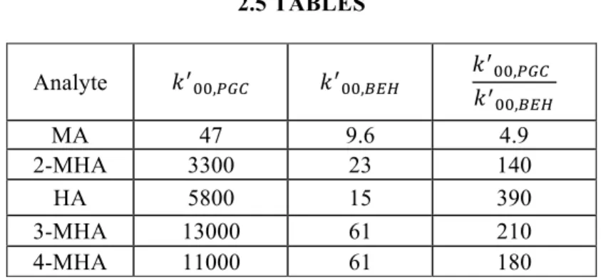
Table 2-1. Projected retention of standard metabolites in 100% water (!! !!) on
Hypercarb (4.6 mm x 100 mm, 3 µm) and C18 BEH (2.1 mm x 50 mm, 1.7 µm) columns as well as the ratio of !!!!,!"#!
!!!!,!"#. Retention was measured over a range of mobile phase compositions consisting of (v/v) mixtures of water/MeOH + 0.1% FA at 30 °C. Experimental retention data was then fit with Equation 2-8 to find !!
!!.!!!!!,!"# and !!!!,!"# are the retention factors in injected
sample solvent for Hypercarb and C18 BEH..……….39 Table 2-2. Data predicting the injection focusing capabilities of packed capillary
C18 BEH and Hypercarb columns assuming a 2 µL injection of standard metabolites in 95/5 (v/v) water/MeOH + 0.1% FA. !!
! data obtained by fitting the experimental retention data on Hypercarb (4.6 mm x 100 mm, 3 µm) and C18 BEH (2.1 mm x 50 mm, 1.7 µm) columns at 30 °C with Equation 2-8. !!
!,!"# and !!!,!"# are the retention factors in injected sample solvent
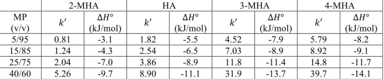
for Hypercarb and C18 BEH.………...40 Table 2-3. Mobile phase composition, !′ (at 30 °C), and ∆!° for C18 BEH
(2.1 mm x 50 mm, 1.7 µm). Values for !′ and ∆!° were determined from van’t Hoff plots, where retention was measured at a range of temperatures. Multiple mobile phase (MP) compositions were used in order to monitor ∆!° under various retention conditions. Mobile phases were (v/v) compositions
of water/MeOH + 0.1% FA. ………41 Table 2-4. Mobile phase composition, !′ (at 30 °C), and ∆!° for Hypercarb
(4.6 mm x 100 mm, 3 µm). Values for !′ and ∆!° were determined from van’t Hoff plots, where retention was measured at a range of temperatures. Multiple mobile phase (MP) compositions were used in order to monitor ∆!° under various retention conditions. Mobile phases were (v/v) compositions of
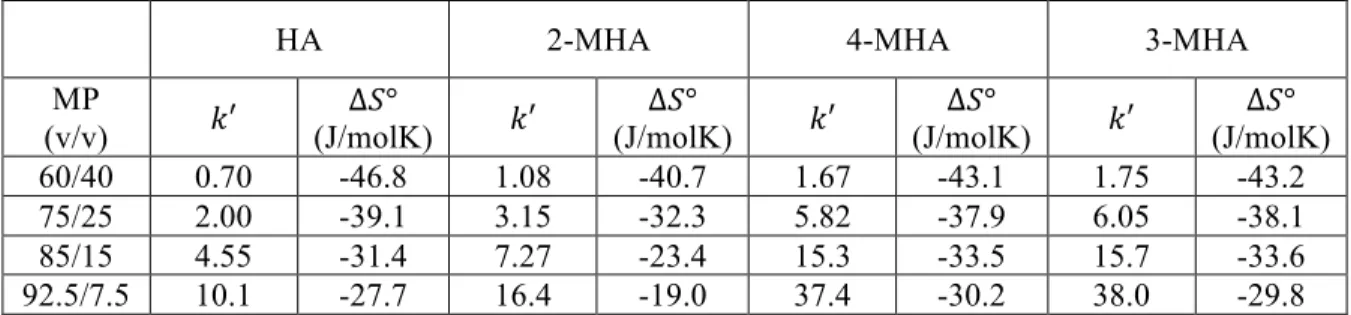
water/MeOH + 0.1% FA. ………42 Table 2-5. Mobile phase composition, !′ (at 30 °C), and ∆!° for C18 BEH
(2.1 mm x 50 mm, 1.7 µm). Values for !′ and ∆!° were determined from van’t Hoff plots, where retention was measured at a range of temperatures. ∆!° was calculated from the intercept of those plots assuming !!= 1. Multiple mobile phase (MP) compositions were used in order to monitor ∆!° under various retention conditions. Mobile phases were (v/v) compositions
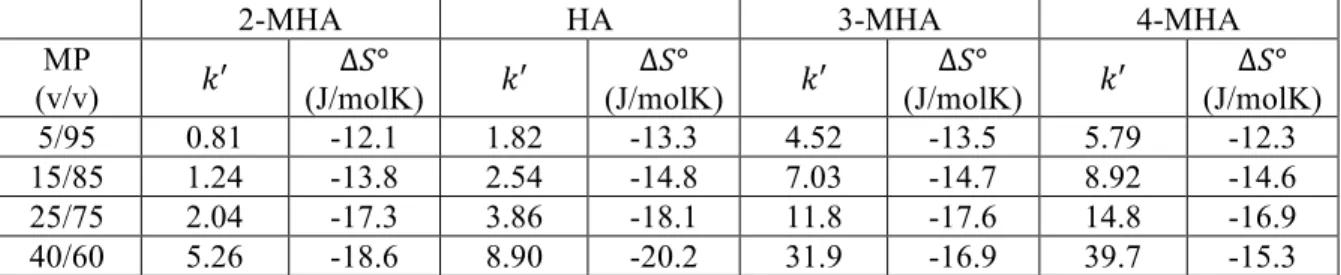
of water/MeOH + 0.1% FA. ………...43 Table 2-6. Mobile phase composition, !′ (at 30 °C), and ∆!° for Hypercarb
(4.6 mm x 100 mm, 3 µm). Values for !′ and ∆!° were determined from van’t Hoff plots, where retention was measured at a range of temperatures. ∆!° was calculated from the intercept of those plots assuming !!= 1. Multiple mobile phase (MP) compositions were used in order to monitor ∆!° under various retention conditions. Mobile phases were (v/v)
compositions of water/MeOH + 0.1% FA. ………..44
Table 3-1. Measured values for !′, !!, !!"", !!!!, and !!!!
conditions used for the C18 BEH column (2.1 mm x 50 mm, 1.7 µm) at 30 °C. !! values determined by dual-UV measurements and adjusted to 30 °C. !!"" determined from plots of the change in spatial variance of all analytes as a function of stop time. Mobile phase compositions were (v/v) mixtures of
water/MeOH + 0.1% FA..………69
Table 3-2. Measured values for !′, !!, !!"", !!!!,and! !!!!
!!!!!along with the conditions used for the Hypercarb column (4.6 mm x 100 mm, 3 µm) at 30 °C.
!! values determined by dual-UV measurements and adjusted to 30 °C.
!!"" determined from plots of the change in spatial variance of all analytes
as a function of stop-flow time. Mobile phase compositions were (v/v) mixtures
of water/MeOH + 0.1% FA. ………70
Table 3-3. Measured values for !′, !!, !!"", !!!!,and!!!!!!
!!!!along with the conditions used for the Hypercarb column (4.6 mm x 100 mm, 3 µm) at 55 °C. !!
values determined by dual-UV measurements and adjusted to 55 °C. !!"" determined from plots of the change in spatial variance of all analytes as a function of stop-flow time. Mobile phase compositions were (v/v) mixtures
of water/MeOH + 0.1% FA. ………71 Table 3-4. Values for slope, intercept and R2 for the linear fit of !
!"! ,! vs !!"#$ for the peak parking experiments using the C18 BEH column (2.1 mm x 50 mm, 1.7 µm) at 30 °C. Analyte and mobile phase conditions are included. Slope values were
changed to units of cm2/s. Based on Equation 3-21, the slope of these trend lines are equal to 2!!"". Mobile phase compositions were (v/v) mixtures of
water/MeOH + 0.1% FA..………72 Table 3-5. Values for slope, intercept and R2 for the linear fit of !
!",!! vs !!"#$ for the peak parking experiments using the Hypercarb column (4.6 mm x 100 mm, 3 µm) at 30 °C. Analyte and mobile phase conditions are included. Slope values
were changed to units of cm2/s. Based on Equation 3-21, the slope of these trend lines are equal to 2!!"". Mobile phase compositions were (v/v)
mixtures of water/MeOH + 0.1% FA. ……….73 Table 3-6. Values for slope, intercept and R2 for the linear fit of !!"! ,! vs !!"#$ for the
peak parking experiments using the Hypercarb column (4.6 mm x 100 mm, 3 µm) at 55 °C. Analyte and mobile phase conditions are included. Slope values
were changed to units of cm2/s. Based on Equation 3-21, the slope of these trend lines are equal to 2!!"". Mobile phase compositions were (v/v)
mixtures of water/MeOH + 0.1% FA..……….74 Table 4-1. Fit parameters for retention of standard metabolites when data from
Figure 4-2 (A) was fit with Equation 4-5 for Hypercarb column (4.6 mm x 100 mm, 3 µm). Retention data measured over a range of water/MeOH + 0.1% FA mobile phases. This data is used for modeling of
Figure 4-2 (B) was fit with Equation 4-5 for C18 BEH column (2.1 mm x 50 mm, 1.7 µm). Retention data measured over a range of water/MeOH + 0.1% FA mobile phases. This data is used for modeling of
gradient separations. Column temperature: 30 °C. Flow rate: 0.3 mL/min.………99 Table 4-3. Column dimensions, gradient conditions, and instrumental parameters
used to model C18 BEH gradients. The gradients being modeled were 5-50% MeOH and 5-30% MeOH, both in 30 minutes. Total column porosity was set such that the predicted deadtime was equal to the experimental deadtime. Data was used in conjunction with standard metabolite retention parameters
from Table 4-2 to model C18 BEH gradients………...……….100 Table 4-4. Comparison of predicted and experimentally measured retention
times for C18 BEH gradient separations. Model chromatogram can be seen in Figure 4-3. Experimental separations (Figure 4-5) were collected using a C18 BEH column (2.1 mm x 50 mm, 1.7 µm) and gradient conditions of 5-50% MeOH as well as 5-30% MeOH, both in 30 minutes. Due to the overlapping retention times of 4-MHA and 3-MHA, only a single retention time was used for the peak. As 4-MHA elutes earlier than 3-MHA, its retention time was chosen as the maxima of the latest eluting peak. Column temperature: 30 °C.
Flow rate: 0.3 mL/min. Retention times used for calculating % difference were the average of multiple identical runs. % difference =!!"#$!!!"#$
!!"#$ where !!"#$ is the experimentally measured retention time and !!"#$ is the
predicted retention time..………101 Table 4-5. Column dimensions, gradient conditions, and instrumental parameters
used to model the Hypercarb gradient. The gradients being modeled were 5-95% MeOH in 90 minutes. Total column porosity was set such that the predicted deadtime was equal to the experimental deadtime. Data was used in conjunction with standard metabolite retention parameters
from Table 4-1 to model Hypercarb gradients..……….102 Table 4-6. Predicted and experimentally measured retention times for Hypercarb
gradient separations. Model chromatogram can be seen in Figure 4-4. Parameters used for modeling can be found in Table 4-5. Experimental
separations were collected using a Hypercarb column (4.6 mm x 100 mm, 3 µm) and a gradient of 5-95% MeOH in 90 minutes at 30 °C and 1 mL/min.
Redox washing conditions are labeled within the table. Retention times
were the average of multiple identical runs..………..103 Table 4-7. Percent difference of predicted and experimentally measured retention
times for Hypercarb gradient separations. Model chromatogram can be
seen in Figure 4-4. Experimental separations were collected using a Hypercarb column (4.6 mm x 100 mm, 3 µm) and a gradient of 5-95% MeOH in 90 minutes at 30 °C and 1 mL/min. Redox washing conditions are labeled within the table. Retention times used for calculating percent difference were the average of multiple identical runs. % difference =!!"#$!!!"#$
!!"#$ where !!"#$ is the experimentally measured retention time and !!"#$ is the
Table 5-1. ℎ!"#, !!"#, Φ, !, !, ! terms from fitting the reduced van Deemter curves of all Hypercarb and BEH columns discusses. All Hypercarb columns were packed using 25 mg/mL slurries in acetone and characterized using electrochemical detection (-0.2 V vs. Ag/AgCl) of BQ in 5/95 water/MeCN + 0.1% FA. C18 BEH column shown for comparison to a traditional reversed phase material. C18 BEH column was characterized using electrochemical detection (+1.1 V vs. Ag/AgCl) of HQ in 50/50 water/MeCN + 0.1% TFA. Flow resistance was not reported for the C18 BEH column, as it is not a
suitable comparison across particle types. ……….141 Table 5-2. Separation window, peak width and peak capacities obtained for the
gradient separation of pooled urine sample using C18 BEH, one-meter
Hypercarb, and two-meter Hypercarb columns. Peak capacities were calculated using Equation 5-1. Reported values are an average of three runs for each column. C18 BEH column: 30.1 cm x 75 µm i.d. packed with 1.9 µm particles. Hypercarb columns: 100 or 200 cm x 75 µm i.d. packed with 3.48 µm
particles. 27 µL gradient from 5-90% MeCN used for C18 BEH and one-meter Hypercarb columns. 54 µL gradient from 5-90% MeCN
LIST OF FIGURES
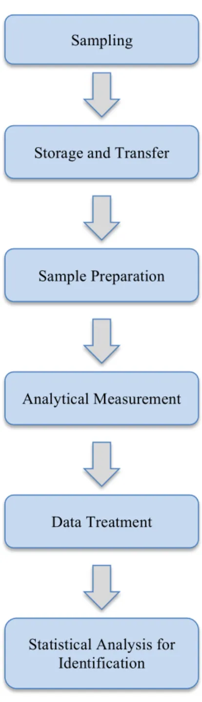
Figure 1-1. Workflow of a standard metabolomics experiment. The specific steps within each process will vary depending on the sample, analysis method, as
well as the overall goal of the analysis.………...……….13 Figure 1-2. Diagram showing the impact of PREG on the electron density when
a negatively (A) and positively (B) charged species approach the PGC surface. Image forces are produced due to the attraction/repulsion of valence electrons
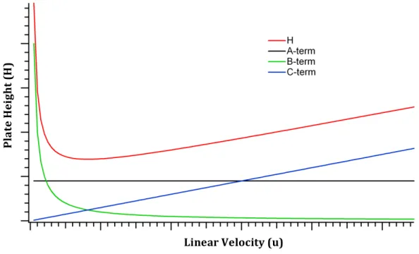
on the particle surface to the analyte………14 Figure 1-3. Contributions of the !, !, and !-terms to the overall plate height,
as a function of linear velocity. These contributions are derived from
Equation 1-3.………15 Figure 1-4. Theoretical plots of plate height vs. linear velocity for columns
packed with 5 µm, 3 µm, and 1 µm particles. It is seen that as the particle diameter decreases, plate height decreases and the minimum plate height
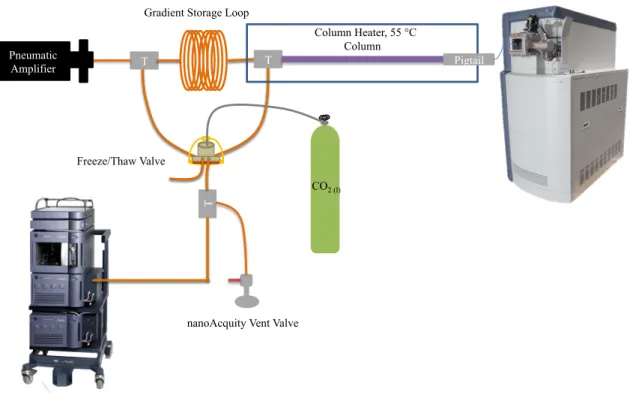
shifts to higher linear velocities.………...16 Figure 1-5. Schematic of the gradient UHPLC system used for capillary
LC-MS analysis. This figure was used with permission from the author. ………...17 Figure 2-1. Chromatograms showing the change in day-to-day repeatability for the
standard test mixture before (A) and after (B) treatment using 10 mM ascorbic acid. Column was 4.6 mm x 100 mm packed with 3 µm Hypercarb. Mobile phase conditions were 5/95 (v/v) water/MeOH + 0.1% FA at a flow rate of 1 mL/min and 30 °C. For (A), measurements were taken over the course of 2 weeks at day 1 (red), day 4 (black) and day 14 (blue). For (B), ascorbic acid treatment was performed before use each day by flowing 10 mM ascorbic acid in mobile phase overnight. Before measurements, ascorbic acid was washed off the column by flushing with mobile phase. Measurements were taken over a similar time span as in (A). Elution order: mandelic acid, 2-MHA, hippuric acid,
3-MHA, and 4-MHA. UV Detection: 240 nm.………45 Figure 2-2. Chromatograms showing the drift in retention over the course of
a single day for 5/95 (v/v) water/MeOH + 0.1% FA (A) and 35/65 (v/v) water/MeOH + 0.1% FA (B) after AA treatment of a Hypercarb column (4.6 mm x 100 mm, 3 µm). Measurements made at a flow rate of 1 mL/min and at 30 °C. Four repeated measurements were taken in sequential order of injection 1 (red), Injection 2 (black), injection 3 (green), and injection 4 (blue). Ascorbic acid treatment was performed before use by flowing 10 mM ascorbic acid in mobile phase overnight.Before measurements, ascorbic acid was washed off column by flushing with mobile phase. Elution order: mandelic acid, 2-MHA, hippuric acid,3-MHA, and 4-MHA.
UV Detection: 240 nm. ………..46 Figure 2-3. Chromatograms showing the change in day-to-day repeatability over
+ 0.1% FA at a flow rate of 1 mL/min and 30 °C. Three measurements were taken over the course of 2 weeks and are overlaid here. Column
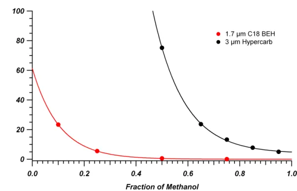
used was new out of box and a different one than used for Figure 2-1 (B)……….47 Figure 2-4. Retention factor of 4-methylhippuric acid on C18 BEH (red)
and Hypercarb (black) columns as a function of methanol volume fraction in the mobile phase. Columns were 2.1 mm x 50 mm packed with 1.7 µm C18 BEH and 4.6 mm x 100 mm packed with 3 µm Hypercarb. Mobile phases consisted of mixtures of (v/v) water/MeOH + 0.1% FA at 30 °C.
Experimental data fit with exponential curves. ………...48 Figure 2-5. Plot of natural log of retention factors of the model metabolites as a
function of methanol volume fraction in the mobile phase on the Hypercarb (A) column (4.6 mm x 100 mm, 3 µm) and C18 BEH (B) column
(2.1 mm x 50 mm, 1.7 µm). Measurements made in (v/v) water/MeOH
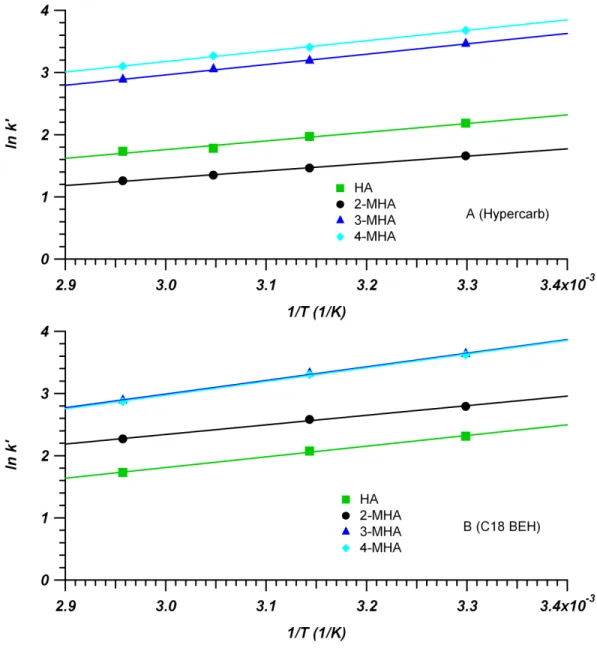
+ 0.1% FA mobile phases at 30 °C. Experimental data fit with Equation 2-8……….49 Figure 2-6. van’t Hoff plots of standard metabolites for Hypercarb
(A, 4.6 mm x 100 mm, 3 µm) and C18 BEH (B, 2.1 mm x 50 mm, 1.7 µm) columns. Mobile phase compositions were 40/60 water/MeOH + 0.1% FA for Hypercarb and 92.5/7.5 water/MeOH + 0.1% FA for C18 BEH. Retention was measured at a number of temperatures between 30 °C and 65 °C. Based on Equation 2-6, the slope is equal to !∆!°! while the intercept is
equal to ∆!!°+ln!. ……….50
Figure 2-7. Plots showing the change in ∆!°, ∆!°, and −!∆!° for 2-MHA (A),
HA (B), 3-MHA (C) and 4-MHA (D) on a C18 BEH (2.1 mm x 50 mm, 1.7 µm) column at various !′. !′ values were determined at 30 °C (also used for !). Values for ∆!° determined using data from Tables 2-3 and 2-5 along
with Equation 2-5………51 Figure 2-8. Plots showing the change in ∆!°, ∆!°, and −!∆!° for 2-MHA (A), HA (B),
3-MHA (C) and 4-MHA (D) on a Hypercarb (4.6 mm x 100 mm, 3 µm) column at various !′. !′ values were determined at 30 °C (also used for !). Values for ∆!° determined using data from Tables 2-4 and 2-6 along
with Equation 2-5……….52 Figure 3-1. Dual UV setup for !! determination studies. Pressure is applied to
the sample vessel, forcing dilute sample in mobile phase through the
capillary. !! calculated using Equations 3-16, 3-17, and 3-18………...75 Figure 3-2. Mobile phase diffusion coefficient measurement for 4-methylhippuric
acid in 5/95 (v/v) water/MeOH + 0.1% FA performed using a capillary, dual-UV setup. Raw signal (red) is sigmoidal due to analyte fronts passing by the two detectors. These sigmoidal curves are differentiated into Gaussian peaks (black) in order to calculate !! from the change in variance between t
he peaks using Equations 3-16, 3-17, and 3-18. UV settings: 240 nm,
!! measurements with measured diameter marked for the vertical and
horizontal axes. Section was clipped from the end of the capillary, so may not be representative of the diameter between detectors, but allows for
comparison to the !! found via calibration with ferricyanide and ferrocyanide………..77 Figure 3-4. Example peak after a peak-parking time of 20 minutes for 2-MHA
in 5/95 water/MeOH + 0.1% FA on the Hypercarb column
(4.6 mm x 100 mm, 3 µm) at 30 °C. Peak shows significant tailing that
could not be accurately fit using the traditional method of ISM………..78 Figure 3-5. Change in spatial variance of all analytes as a function of stop time for
C18 BEH at 30 °C (A), Hypercarb at 30 °C (B) and Hypercarb at 55 °C (C). Based on Equation 3-22, the slope of these trend lines are equal to 2!!"".
In order to cover a range of retention factors, different analytes and
mobile phase conditions were used.……….79 Figure 3-6. Comparison of !!!! for C18 BEH at 30 °C (red), Hypercarb at
30 °C (black), and Hypercarb at 55 °C (green) as a function of analyte retention factor. The choice of analyte and mobile phase composition were varied in order to cover a wide range of retention factors for each column. Error bars are shown for each data point. In-depth discussion of error
calculation can be found in the Appendix. ………..80 Figure 3-7. Comparison of !!!! !!!! as a function of retention factor for C18
BEH (red) at 30 °C, Hypercarb at 30 °C (black) and Hypercarb at 55 °C (green). The choice of analyte and mobile phase composition were varied in order to cover a wide range of retention factors for each column. Error bars are shown for each data point. In-depth discussion of error calculation can be
found in the Appendix. ………81 Figure 4-1. Gradient chromatogram used to determine the system dwell volume.
Gradient went from 100% mobile phase A (water) to 100% mobile phase B (water + 0.1% acetone) in five minutes. A short length of capillary was used to connect the injector and detector to minimize any extra volume
contributions. Flow rate was 50 µL/min. To calculate !!"#$$, it was necessary to find the time at which the acetone intensity reached 50% of its
maximum (!!/!) for use with Equations 4-3 and 4-4. !!/! is marked
on the plot (4.09 minutes).………105 Figure 4-2. Plot of log of retention factors of the model metabolites as a function of
methanol volume fraction in the mobile phase on the Hypercarb
(A, 4.6 mm x 100 mm, 3 µm) and C18 BEH (B, 2.1 mm x 50 mm, 1.7 µm)
columns. Measurements made in water/MeOH + 0.1% FA mobile phases at 30 °C,
Experimental data, which was discussed in Chapter 2, was fit with Equation 4-5…………106 Figure 4-3. Predicted gradient chromatograms for metabolites on C18 BEH.
Predicted retention times can be found in Table 4-4………..107 Figure 4-4. Predicted gradient chromatogram for metabolites on Hypercarb. Prediction
based off of isocratic retention data (Table 4-1) and gradient parameters (Table 4-5). Gradient conditions: 5-95% MeOH in 90 minutes. Column: 4.6 mm x 100 mm, 3 µm Hypercarb. Assumed flow rate: 1 mL/min.
Predicted retention times can be found in Table 4-6..………108 Figure 4-5. Gradient separations of model metabolites on C18 BEH using gradients
of 5-50% MeOH (A) and 5-30% MeOH (B), both in 30 minutes. Column: 2.1 mm x 50 mm, 1.7 µm C18 BEH. Wavelength: 240 nm. Column temperature:
30 °C. Flow rate: 0.3 mL/min. Retention times can be seen in Table 4-4..………...109 Figure 4-6. Sequential gradient separations of model metabolites on Hypercarb with
10 mM ascorbic acid treatment only before the first run. Gradient conditions: 5-95% methanol in 90 minutes. Column: 4.6 mm x 100 mm, 3 µm Hypercarb. Wavelength: 240 nm. Column temperature: 30 °C. Flow rate: 1 mL/min. The order of runs was black (first), green (second) and then red (third).
Retention times can be seen in Table 4-6..……….110 Figure 4-7. Replicate gradient separations of model metabolites on Hypercarb with
10 mM ascorbic acid treatment between runs. Gradient conditions: 5-95% methanol in 90 minutes. Column: 4.6 mm x 100 mm, 3 µm Hypercarb. Wavelength: 240 nm. Column temperature: 30 °C. Flow rate: 1 mL/min. The large signal at the beginning of the runs is due to ascorbic acid washing off of the column from the treatment
step performed before the run started. Retention times can be seen in Table 4-6…………..111 Figure 4-8. Replicate gradient separations of model metabolites on Hypercarb with
100 µM ascorbic acid in the mobile phase. Gradient conditions: 5-95% methanol with 100 µM ascorbic acid added, in 90 minutes. Column:
4.6 mm x 100 mm, 3 µm Hypercarb. Wavelength: 240 nm. Column temperature: 30 °C. Flow rate: 1 mL/min. The large peak at the beginning of the runs is due to ascorbic acid washing off of the column. Retention times can be seen
in Table 4-6………..………..112 Figure 4-9. Replicate gradient separations of model metabolites on Hypercarb
with 50 µM ascorbic acid in the mobile phase. Gradient conditions: 5-95% methanol with 50 µM ascorbic acid added, in 90 minutes. Column:
4.6 mm x 100 mm, 3 µm Hypercarb. Wavelength: 240 nm. Column temperature: 30 °C. Flow rate: 1 mL/min. The large peak at the beginning of the runs is due to ascorbic acid washing off of the column. Retention times can be seen
in Table 4-6………113 Figure 4-10. Replicate gradient separations of model metabolites on Hypercarb with
1 µM ascorbic acid in the mobile phase. Gradient conditions: 5-95% methanol with 1 µM ascorbic acid added, in 90 minutes. Column: 4.6 mm x 100 mm, 3 µm Hypercarb. Wavelength: 240 nm. Column temperature: 30 °C.
Flow rate: 1 mL/min. Retention times can be seen in Table 4-6. ………..114 Figure 4-11. Replicate gradient separations of model metabolites on Hypercarb with 500
with 500 µM sodium sulfite added, in 90 minutes. Column: 4.6 mm x 100 mm, 3 µm Hypercarb. Wavelength: 240 nm. Column temperature: 30 °C. Flow rate:
1 mL/min. Retention times can be seen in Table 4-6..………...115 Figure 5-1. Schematic of the gradient UHPLC system used for capillary LC-MS
analysis. This figure was used with permission of the author. ………..143 Figure 5-2. Gradient profile for the separation of human urine metabolites on the
C18 BEH and one-meter Hypercarb columns. 27 µL gradient volume going from 5 to 90% MeCN. Note that this gradient is loaded in reverse so that
it is pushed through the column in the correct order. ………144 Figure 5-3. Example image of Hypercarb particle population used for capillary
columns (A) and the histogram of particle distribution (B) with average and relative standard deviation in plot. Particles diameter was measured using ImageJ software. A total of 783 particles were measured for the population
presented here. ………...145 Figure 5-4. SEM image of extruded Hypercarb bed after flushing with 55,000 psi.
The original column was packed with sonication, in order to expose the particles to the harshest conditions they may experience during the process. Column was flushed in 5/95 water/MeCN + 0.1% FA, after which the inlet
region of the bed was extruded for imaging………...146 Figure 5-5. Chromatograms showing the detection of hydroquinone and
1,4-benzoquinone on C18 BEH (A) and Hypercarb (B) capillary columns using electrochemical detection. For the C18 BEH column, the oxidation of HQ was detected while the electrode was at +1.1 V (ascorbic acid also injected in sample). As BQ is the oxidized species of HQ, it was necessary to change the electrode potential to -0.2 V for detection (opposite signal directions due to oxidative vs. reductive current). For PGC, HQ was not detected at +1.1 V, but rather when either BQ or HQ was injected onto the Hypercarb column, an identical reduction current observed (electrode at -0.2 V). C18 BEH
mobile phase: 50/50 water/MeCN + 0.1% TFA. Hypercarb mobile phase:
5/95 water/MeCN + 0.1% FA..………..147 Figure 5-6. UV spectra measured for BQ and HQ in 5/95 water/MeCN + 0.1% FA (A),
chromatogram showing BQ and HQ being injected separately onto a standard bore Hypercarb column (4.6 mm x 100 µm, 3 µm) with PDA detection (B) and corresponding UV spectra after being analyzed by Hypercarb column
for each analyte (C). Flow rate: 1 mL/min. 30 °C.……….148 Figure 5-7. Chromatogram of samples containing acetone and hydrogen peroxide
as potential deadtime markers using UV detection. Column was 100 cm x 75 µm i.d. packed with 3.48 µm Hypercarb. Mobile phase: 5/95 water/MeCN + 0.1% FA. Identical retention times of acetone and hydrogen peroxide suggest H2O2 acts as a deadtime marker. !! of BQ in 5/95 water/MeCN + 0.1% FA
was 0.4..……….……….………149 Figure 5-8. Reduced van Deemter plots of 1,4-benzoquinone for duplicate, 2 m
sonication during the packing process. 25 mg/mL slurry in acetone used for all columns. Squares and circles are used to differentiate between the two columns from each condition. All columns were 200 cm x 75 µm i.d. packed with 3.48 µm Hypercarb and characterized using electrochemical detection (-0.2 V vs. Ag/AgCl) of BQ (!! ~0.4) at the outlet. Mobile phase:
5/95 water/MeCN + 0.1% FA………150 Figure 5-9. Reduced van Deemter plots of 1,4-benzoquinone for comparison of
one (green) and two-meter (red) packed Hypercarb columns when packed without sonication during the packing process. A comparative C18 BEH column is shown in blue. 25 mg/mL slurry in acetone used for all Hypercarb columns. Squares and circles are used to differentiate between the two columns from each condition. Hypercarb columns were either 100 cm or 200 cm x 75 µm i.d. packed with 3.48 µm particles and characterized using electrochemical detection (-0.2 V vs. Ag/AgCl) of BQ (!! ~0.4) at the outlet with 5/95
water/MeCN + 0.1% FA. C18 BEH column was 30.1 cm x 75 µm i.d. packed with 1.9 µm particles and characterized using electrochemical detection (+1.1 V vs. Ag/AgCl) of HQ (!! ~0.2) at the outlet with 50/50
water/MeCN + 0.1% TFA………..151 Figure 5-10. Gradient separations of single donor urine using C18 BEH (A) and
Hypercarb (B) columns. Identical gradient conditions (27 µL from 5-90% MeCN) were used for both columns to allow direct comparison of retention times.
Separations performed at 55 °C. Pressure was adjusted to make flow rate 300 nL/min for each column in gradient initial conditions. C18 BEH column: 30.1 cm x 75 µm i.d., 1.9 µm particles. Hypercarb column:
100 cm x 75 µm, 3.48 µm particles………152 Figure 5-11. Two dimensional plots of the gradient separations of single donor urine
using C18 BEH (A) and Hypercarb (B) columns, showing m/z vs. time. 27 µL gradient from 5-90% MeCN was used for C18 BEH and one-meter Hypercarb columns. Separations performed at 55 °C. Pressure was adjusted to make flow rate 300 nL/min for each column. C18 BEH column: 30.1 cm x 75 µm i.d., 1.9 µm particles. Hypercarb column: 100 cm x 75 µm, 3.48 µm particles. Circled regions show patterning of increase m/z, suggesting possible polymer
contamination from sample preparation process………153 Figure 5-12. Gradient separations of pooled urine using C18 BEH (A), one-meter
Hypercarb (B) and two-meter Hypercarb (C) columns. 27 µL gradient from 5-90% MeCN was used for C18 BEH and one-meter Hypercarb columns. 54 µL gradient used for two-meter Hypercarb column. Separations performed at 55 °C. Pressure was adjusted to make flow rate 300 nL/min for each column in gradient initial conditions. C18 BEH column: 30.1 cm x 75 µm i.d., 1.9 µm
particles. Hypercarb column: 100 or 200 cm x 75 µm, 3.48 µm particles……….154 Figure 5-13. Two-dimensional plots of the gradient separations of pooled
urine using C18 BEH showing m/z vs. time. Chromatogram can be seen in
Figure 5-12 (A). C18 BEH column: 30.1 cm x 75 µm i.d., 1.9 µm particles……….155
seen in Figure 5-12 (B). Hypercarb column: 100 cm x 75 µm,
3.48 µm particles………156 Figure 5-15. Two-dimensional plots of the gradient separations of pooled urine
using two-meter Hypercarb column showing m/z vs. time. Chromatogram can be seen in Figure 5-12 (C). Hypercarb column: 200 cm x 75 µm,
LIST OF ABBREVIATIONS
2-MHA 2-methylhippuric acid
3-MHA 3-methylhippuric acid
4-MHA 4-methylhippuric acid
A/D Analog-to-digital
AA Ascorbic acid
Ag/AgCL Silver/silver chloride
BEH Bridged-ethyl hybrid
BQ 1,4-Benzoquinone
C18 n-Octadecyl
CLSM Confocal laser scanning microscopy EMG Exponentially-modified Gaussian
ESI Electrospray ionization
FA Formic acid
GC-MS Gas chromatography-mass spectrometry
HA Hippuric acid
HILIC Hydrophobic interaction liquid chromatography HPLC High performance liquid chromatography
HQ Hydroquinone
i.d. Inner diameter
IFF Isocratic-focusing factor
ISM Iterative statistical moments
KCl Potassium chloride
LC Liquid chromatography
LC-MS Liquid chromatography-mass spectrometry
MeCN Acetonitrile
MeOH Methanol
MP Mobile phase
MS Mass Spectrometry
m/z Mass-to-charge ratio
NMR Nuclear magnetic resonance
o.d. Outer diameter
PDA Photodiode array
PGC Porous graphitic carbon
POISe Performance optimizing injection sequence PREG Polar retention effect on graphite
qToF Quadrupole time-of-flight RSD Relative standard deviation SEM Scanning electron microscopy TASF Temperature assisted solute focusing
TFA Trifluoroacetic acid
UHPLC Ultra-high pressure liquid chromatography UPLC Ultra-performance liquid chromatography
UV Ultraviolet
LIST%OF%SYMBOLS%
! Eddy diffusion van Deemter term
!!"#$ Amplitude of Exponentially Modified Gaussian function peak fit
! Reduced eddy diffusion van Deemter term
!!"#$% Parameter allowing for observed curvature in the fit of retention data
! Longitudinal diffusion van Deemter term
!!"# Solute dependent term largely determined by molecular weight
! Reduced longitudinal diffusion van Deemter term
! Resistance to mass transfer van Deemter term
! Reduced resistance to mass transfer van Deemter term
!!"" Effective diffusion coefficient
!!"",!!"# Effective diffusion coefficient of 2-methylhippuric acid
!!"",!"#$%&# Effective diffusion coefficient of acetone
!! Diffusion coefficient of an analyte in the mobile phase
!!,! Frequency factor of mobile phase diffusion
!!,!!"# Diffusion coefficient of an 2-methylhippuric acid in the mobile phase
!!,!"#$%&# Diffusion coefficient of an acetone in the mobile phase
!! Stationary phase diffusion coefficient !!,! Frequency factor of surface diffusion
!! Column inner diameter
!!"#,! Distance that an unretained analyte travels over the course of injection
loading
!!"#,! Distance that a retained analyte travels over the course of injection loading
!! Particle diameter
!! Activation energy of molecular diffusion in the stationary phase
! Volumetric flow rate
! ! Measured peak signal in the time domain
∆!° Standard Gibbs free-energy
! Gradient compression factor
! Gradient slope
! Height equivalent of a theoretical plate
∆!° Standard enthalpy of transfer from mobile to stationary phase
ℎ Reduced plate height
ℎ!"#! Minimum reduced plate height
!""!"# Isocratic-focusing factor on C18 BEH column
!""!"# Isocratic-focusing factor on Hypercarb column
!! Frequency factor of adsorption
! Analyte partition coefficient
!!"# Term describing the injection profile
!!
!! Retention factor of an analyte in 100% water
!!
!!,!"# Retention factor of an analyte in 100% water for C18 BEH column
!!
!!,!"# Retention factor of an analyte in 100% water for Hypercarb column
!! Analyte retention factor
!!
! Analyte retention factor in a specific mobile phase composition !!
!,!"# Analyte retention factor in a specific mobile phase composition for C18 BEH
column
!!
!,!"# Analyte retention factor in a specific mobile phase composition for
Hypercarb column
!! Boltzmann constant
!!
!!"!#$! Combined term definining the retention of a solute for error propogation
! Length of a chromatographic column
!! Molecular weight of a solute
! Number of theoretical plates
!!"# Number of theoretical plates at the optimum velocity
!!"#,!! Number of theoretical plates at the optimum velocity for a 1 m
Hypercarb column
!!"#,!! Number of theoretical plates at the optimum velocity for a 2 m
Hypercarb column
!! Peak capacity
!!,!! Peak capacity for a 1 m Hypercarb column
!!,!! Peak capacity for a 2 m Hypercarb column
∆! Required pressure drop
∆!!"# Pressure required to reach the optimum linear velocity of a column
!!" Isosteric heat of adsorption
! Gas constant
!! Hydrodynamic radius of a solute
! Constant dependent on solute molecular weight
∆!° Standard entropy of transfer from mobile to stationary phase
! Absolute temperature
!!/! Time to reach 50% of maximum signal intensity
! Time
!!"#$% Gradient delay time
!!"#$ Experimentally measured retention time
!! Gradient length in time
!!"# Time it takes to load a fixed injection volume
!! Column deadtime
!!"#$ Predicted retention time
!! Retention time of an analyte
!!"#$ Stop time
!" Time between detected peaks
! Linear velocity of the mobile phase
!! Solute linear velocity
!! Total volume a solute band occupies after injection loading
!!,!"# Total volume a solute band occupies after injection loading on C18 BEH
column
!!,!"# Total volume a solute band occupies after injection loading on Hypercarb
column
!!"#$$ Dwell volume
!! Solvent Free volume
!!"# Injection volume
!! Volume of mobile phase in the column
!!"# Maximum allowable injection volume
!! Volume of stationary phase in the column
! Reduced linear velocity
!! Average peak width
β Surface diffusion fraction of isosteric heat of adsorption
!! Mobile phase obstruction (tortuosity) factor !! Stationary phase obstruction (tortuosity) factor
!! Interparticle porosity of the column
! Mobile phase viscosity
! Term related to the amount of allowable performance loss from injection
!!"## Distance between two equilibrium positions for diffusion
!!!!! Standard deviation of the term, retention factor plus one
!!"!,! Spatial variance of a peak due to longitudinal diffusion
!!!"" Standard deviation of the analyte effective diffusion coefficient
!!!""!! Standard deviation of the analyte effective diffusion coefficient minus
the mobile phase contribution to effective diffusion
!!!"",!"#$%&# Standard deviation of the effective diffusion contribution for acetone
!!!"",!!"# Standard deviation of the effective diffusion for 2-methylhippuric acid
!!!"",!!"#!! Standard deviation of the analyte effective diffusion coefficient minus
the mobile phase contribution to effective diffusion for 2-methylhippuric acid
!!! Standard deviation of the analyte diffusion coefficient in the mobile
phase
!!!,!"#$%&# Standard deviation of the diffusion coefficient of acetone in the
mobile phase
!!!,!!"# Standard deviation of the diffusion coefficient of 2-methylhippuric acid
in the mobile phase
!!!! Standard deviation of the square of the column diameter
!!! Standard deviation of the column diameter
!!! Standard deviation of the retention factor
!!
!"!#$! Standard deviation of the combined term defining the retention of a
solute for error propagation
!!"##! Temporal variance due to longitudinal molecular diffusion
!!"# Sigma parameter from Exponentially Modified Gaussian function peak
fit
!!"#$%,!"#$%&# Standard deviation of the slope for acetone
!!"#$%,!!"# Standard deviation of the slope for 2-methylhippuric acid
!!!! Temporal variance of first detected peak
!!!! Temporal variance of second detected peak
!!! Temporal variance of a peak
!∆! Standard deviation of the migration time between detected peaks !!!,!"𝐺 Variance of peak fit with Exponentially Modified Gaussian function
!!! Standard deviation of the deadtime
!!!_!"# Accumulated temporal variance between detectors
!!! Standard deviation of the retention time
!!!!!! Standard deviation of the time difference between retention time and deadtime
!!! Standard deviation of the mobile phase obstruction factor
!!!!! Standard deviation of the mobile phase obstruction factor times mobile phase phase diffusion coefficient
!!!!!,!!"# Standard deviation of the mobile phase obstruction factor times mobile phase phase diffusion coefficient for 2-methylhippuric acid
!!!!! Standard deviation of the stationary phase obstruction factor times stationary phase diffusion coefficient
!!!!! Standard deviation of the stationary phase obstruction factor times stationary phase diffusion coefficient
! !!!! !!!!
Standard deviation of the stationary phase contribution divided by the mobile phase contribution
! !!!!!
!!!!,!!"#
Standard deviation of the stationary phase contribution divided by the mobile phase contribution for 2-methylhippuric acid
!∆!!_!!"# Standard deviation of the accumulated temporal variance
!!"## Rate constant of diffusion
!!"# Tau parameter from Exponentially Modified Gaussian function peak fit
Φ Flow resistance
! Phase ratio
! Fraction of mobile phase consisting of organic content
∆! Change in organic content over the gradient
! Mobile phase diffusion contribution to the effective diffusion coefficient
CHAPTER 1. INTRODUCTION
1.1 Metabolomics
1.1.1 Scope of Metabolomics Analysis
The field of metabolomics encompasses the detection, quantification, and identification of small molecules (molecular weight < 1,200 Da) produced during cellular processes in biological samples.1 This systems biology level approach of studying metabolism has provided insight into the processes of drug discovery, disease biomarker detection, and toxicology.2–6 The metabolome encompasses a wide variety of compounds including, among other things, amino acids, lipids, fatty acids, vitamins, and carbohydrates. For humans alone, there are over 40,000 confirmed metabolites.7 Analysis of metabolites can be classified into a number of different strategies based on the desired information about the sample. These strategies include targeted analysis, global profiling, clinical diagnostics, and metabolic fingerprinting.8
A general metabolomics workflow can be found in Figure 1-1. The specifics of each step will be determined by the sample, analysis method, and goal of the experiment. For detailed metabolomics studies, hundreds to thousands of samples must be collected and analyzed.6 Small differences in metabolic profile are often being investigated, making the stability of these samples and
1.1.2 Analytical Techniques used for Metabolomics
Metabolomic samples provide a complex analytical problem. Compared to proteomics and transcriptomics, metabolomics offers a much more diverse range of compounds.12 With only 20 amino acid building blocks for the proteome and four nucleotide bases for the transcriptome, the structural variability is limited.12 Increased structural variation leads to more chemical variability in metabolites, as seen by the range in polarities between metabolites such as carbohydrates and lipids. Another complicating factor is that the metabolic profile expressed within a human is not just dependent on their genetics, but also a number of other factors including, but not limited to, diet, chemical exposures, gender, and age.13–16 These factors produce a number of exogenous and
endogenous compounds that are in flux not only over the course of a human lifetime, but also over the course of a single day. The concentration range of species in metabolite samples can also span 9-orders of magnitude (mM to pM), requiring sensitive detection of low abundance species.12
To date, the most common analytical methods used for metabolomics analysis are nuclear magnetic resonance (NMR) spectroscopy, gas chromatography-mass spectrometry (GC-MS), and liquid chromatography-mass spectrometry (LC-MS).12 Due to the complexity of the human metabolome, no single method can provide analysis of all metabolites.17 These techniques provide complimentary information, and can be used in combination to get a more complete picture of the metabolite profile at the time of sampling.
NMR provides the ability to do analysis of metabolite samples with little to no sample preparation in a highly reproducible and non-destructive manner.18,191H NMR is most often used as the majority of metabolites will contain hydrogen atoms, allowing simultaneous detection of a large number of species. Due to the complexity of samples, a single NMR spectrum could produce thousands of signals, providing a great deal of structural information about metabolites after
GC-MS allows for the separation and detection of wide range of low molecular weight and volatile metabolites with low limits of detection. A derivitization step using silylating reagents is needed to allow for sufficient volatility of the polar species.11 The resulting chromatograms can contain hundreds of peaks, which can be correlated to metabolite identifications using deconvolution software and spectral database searching.22 Although GC-MS has been widely utilized for
metabolomics, it does have several shortcomings. First, due to the volatility needed for analysis, GC-MS is inherently biased against high molecular weight and non-volatile species.12 Also, the additional derivitization step needed for polar species adds sample preparation time and is potentially a source of variability if not done in a repeatable fashion.23 Consistency of the derivitization step has been
improved by the development of automated systems, although the process can still lead to multiple peaks for a single compound due to partial, or incomplete derivitization.11,23
LC-MS is capable of analyzing metabolites with a wide range of properties and low limits of detection with the added benefit of not requiring any sample derivitization. Traditionally, reversed phase separations using n-octadecyl (C18) bonded silica particles are used for metabolomics.24–26 The popularity of reversed phase separations is due to its well-understood properties as well as the simplicity of use. Reversed phase columns utilize a hydrophobic particle surface in conjunction with aqueous mobile phases containing low levels of organic content (acetonitrile or methanol).27
Compounds interact with the stationary phase and are retained based on increasing hydrophobicity. Due to the wide range of polarities present in metabolite samples, it is often necessary to utilize gradient separations, where the organic content in the mobile phase is increased over the course of the run. The pitfall with reversed phase columns is their inability to sufficiently retain polar species.28,29 These species will not interact strongly with the C18 layer, ultimately leading to compounds eluting at the pace of the mobile phase or as very wide bands early in the gradient. Metabolite samples are typically derived from aqueous fluids, therefore many of their constituents will be highly polar and when analyzed with a reversed phase column, a loss of information may occur.
columns, hydrophilic interaction liquid chromatography (HILIC) has become more popular for applications such as the analysis of urinary metabolites.29–31 HILIC utilizes a polar stationary phase (bare silica, aminopropyl modified, or diol modified are common) in conjunction with aqueous mobile phases containing a high level of acetonitrile to allow retention and separation of polar species.32 The retention mechanism for HILIC is complex and involves a layer of water that is bound to the particle surface, into which solutes will partition. Although HILIC is able to analyze polar compounds, any metabolite with a moderate amount of hydrophobicity will be unretained. Similar to C18 bonded columns; HILIC columns are not capable of separating the whole range of polarities that are expected in metabolite samples. Therefore, HILIC and reversed phase separations are considered to be complementary in the information that they provide.32,33 As an alterative to these C18 bonded and HILIC columns, porous graphitic carbon has been shown able to retain both non-polar and polar species using a single chromatographic column, potentially providing similar information in
decreased analysis time.34
1.2 Porous Graphitic Carbon
1.2.1 Origin of Porous Graphitic Carbon in Chromatography
Initial interest in carbon as a chromatographic stationary phase was spurred by the knowledge that silica is unstable under basic conditions and high temperatures.27,35 Since the 1970’s, many attempts to produce a chromatographically useful carbon stationary phase have been made. Early on, the primary issues that were encountered were a lack of mechanical stability as well as poor
> 2500 °C under inert conditions, which ordered the carbon structure and eliminated micropores that were previously present. This material was commercialized under the trade name of Hypercarb, and is now available in 7 µm, 5 µm, and 3 µm particle sizes. In 1991, two other groups published alternative methodologies for the production of porous graphitic particles.41,42 These materials were
commercialized as BTR Carbon and TSK-gel Carbon-500. Although the synthetic pathways used to produce these three forms of porous graphitic carbon are different, they all are expected to have similar properties and so they will all be grouped under the title of PGC throughout the following Chapters.
Further studies by Knox, Kaur, and Millward into Hypercarb allowed insight into the structure of the PGC surface.43 PGC particles are composed of intertwined stacks of graphitic sheets of sp2 hybridized carbon atoms, giving the surface a flat structure. The atoms within a single sheet are held together by covalent bonds, while the layers of sheets interact by van der Waals forces. PGC particles are considered two-dimensional graphite, which differs from three-dimensional graphite in that it no longer has regular orientation of the layered graphite sheets. The basal plane of the PGC, or the plane parallel to the graphitic sheets, is atomically flat and has a satisfied valence throughout, making it highly polarizable.44 The carbon atoms on the edge plane, or the plane perpendicular to the sheets, posses an unsatisfied valence and are thought to be sites where oxidizable functional groups could exist.45 While bonded silica based stationary phases are unstable under basic and high
temperature conditions, PGC, being composed completely of carbon, is stable across the full range of pH as well as temperatures up to 200 °C.46–48
1.2.2 Retention Mechanisms of PGC
the addition of a methylene group to a compound produces a larger change in retention on PGC. Overall, the retention of non-polar species tend to be higher on PGC, and has been shown to be due in part to the flat surface favoring strong adsorption of the solutes.
Although PGC is composed solely of carbon, it does not strictly act like a reversed phase system. Early on it was realized that the electronic distribution of the solute impacted its retention.51 Ross and Knox classified these electrostatic interactions with polar compounds as the polar retention effect on graphite (PREG).47 As mentioned previously, the basal plane of the graphite sheets contain delocalized electrons, making the surface highly polarizable. When a polar compound approaches the surface, the electron cloud will form an image force based on the electron density of the polar group. Figure 1-2 is a diagram of the induced dipoles that would be produced on the PGC due to positively and negatively charged groups nearing the surface. As the strength of electrostatic interactions is dependent on the distance between the bodies, it is expected that the orientation of polar functional groups in relation to the graphite surface play a role in retention.52 Although the combination of the dispersive interaction and PREG mechanism allow increased retention of both polar and non-polar species when compared to traditional reversed phase systems, it comes at the cost of added
complexity for understanding the interplays of these mechanisms. 1.2.3 Application of PGC Columns
The main areas of interest that PGC particles have been applied are in the separations of polar analytes and structurally similar analytes. Due to the increased retention of polar compounds with the PREG mechanism, PGC columns have been successfully applied to neurotransmitters, carbohydrates, organic explosives, and glycans.53–56 Since the graphite surface is flat, the three-dimensional
stationary phases.58,59 The utility of PGC to separate polar, non-polar, and structurally similar species with a single column makes it a unique material for a variety of separations. Despite these unique properties, widespread adoption of PGC has been limited due to the complexities of its retention mechanism making the prediction of the elution of solutes a challenge, along with inherent redox properties which have been shown to influence separations (discussed in Chapter 2).34
1.3 Chromatographic Theory 1.3.1 Chromatographic Efficiency
In order to perform quality separations of complex metabolite samples, it is vital to have a highly efficient column. Although gradient separations are typically used with metabolomics samples, it is still useful to determine the efficiency of a column using isocratic separations. While flowing down a chromatographic column under isocratic conditions, a solute band experiences a variety broadening processes that ultimately sum to the final peak profile. The efficiency is determined by direct measurement of the peak profile and its corresponding number of theoretical plates (!).27
!= !!
!
!!! Equation 1-1
Here, !! is the analyte retention time and !!! is the temporal variance of the measured peak. !
provides a dimensionless value describing the overall performance for a single solute, but provides no context of the column used to perform the separation. In order to compare packed columns, the height equivalent of a theoretical plate (!) is a more useful term as it scales ! to the column length (!).
!= !
! Equation 1-2
!=!+!
!+!" Equation 1-3
Here, the !-term describes the contribution of eddy dispersion, the !-term describes the contributions of longitudinal diffusion, and the !-term describes the resistance to mass transfer within the column. Equation 1-3 clearly shows that the broadening processes vary with ! and that they are additive to !, which can be visualized in Figure 1-3.
Although the van Deemter equation allows understanding the plate height variation with mobile phase velocity, it falls short in allowing direct comparison of columns packed with different particle sizes (!!) as well as varying analyte diffusion coefficients in the mobile phase (!!). For this
reason, terms for the reduced plate height (ℎ) and reduced velocity (!) are often calculated using Equations 1-4 and 1-5.60
ℎ= !
!! Equation 1-4
!=!!!
!! Equation 1-5
These terms can also be substituted into Equation 1-3 to form the reduced van Deemter equation.
ℎ=!+!
!+!" Equation 1-6
Here, !, !, and ! are the reduced forms of the broadening terms discussed above. Again, the use of Equation 1-6 allows for direct comparison of the performance of columns of varying lengths, packed with different particle sizes, as well as differing analyte/mobile phase combinations. Detailed mathematical discussion of the van Deemter terms is beyond the scope of this work, but the basic principles of the contributions will be discussed here.61–64
1.3.3 !-term Broadening
leading to a broadening of the band. Giddings’ work described a more complex picture of eddy dispersion involving five different regimes that account for !-term broadening: transchannel, short-range interchannel, long-short-range interchannel, transparticle and transcolumn.61 The difference between these regimes is the distance scale upon which they operate within a packed bed. Although the !-term is considered to be independent of flow in the van Deemter equation, these regimes all will be
partially dependent on linear velocity.63,64 The flow dependence can manifest as an apparent increase in!!-term, disguising the overall contribution of the !-term.64 By improving the homogeneity of the packed bed, the range of flow paths can be reduced, thus stressing the importance of packing a uniform bed structure.62
1.3.4 !-term Broadening
The B-term describes broadening due to longitudinal diffusion within the column, coming about from the relaxation of concentration gradients within the solute band. Increasing linear velocity will reduce the contribution from longitudinal diffusion. There are number of diffusional processes that occur within the column that will broaden the solute band. Diffusion in the mobile phase can occur in the interstices of the particles as well as within the pores of fully porous or superficially porous particles. The mobile phase within the particle pores is also known as the stagnant mobile phase. In practice, the diffusion coefficients in the mobile phase and stagnant mobile phase are some fraction of !! as obstructions due to the particle packed bed as well as possible steric constriction
within the particle pores limit diffusion.61 A third, and often ignored, source of diffusion is that within the stationary phase of the packing material.27 Even when in a retained state, solute molecules can still diffuse along the particle surface, with this contribution becoming potentially more significant for highly retained analytes that spend a lot of time in the stationary phase.65
1.3.5 !-term Broadening
from the mobile and stationary phases, but if porous particles are used, a contribution from the stagnant mobile phase will also be included. Stationary phase resistance to mass transfer comes about due to the time it takes for solutes to diffuse into and out of the stationary phase.27 Mobile phase resistance to mass transfer is related to the transit of analyte from the interparticle volumes to the particle surface.
1.3.6 Effect of Particle Size on Performance
When looking to improve separations, one route to achieve this is by utilizing packing material of differing size. In particular the ! and !-terms scale with !! and !!!, respectively.27 This
means that by utilizing smaller particles, ! will decrease accordingly. Figure 1-4 shows the change in ! that is expected when using 5 µm, 3 µm, and 1 µm particles. Another observation is that as particle
size decreases, the linear velocity at which the minimum plate height is observed is shifted higher. Improvements in column performance when moving to smaller particles is what led to the
development of ultrahigh pressure liquid chromatography (UHPLC) in our lab. The pressure required to flow through a packed bed can be found using the Kozeny-Carman equation:27
∆!= 185!"# !!!
1−!!
!! Equation 1-7
where ∆! is the required pressure drop, ! is the mobile phase viscosity, and !! is the fraction of
column volume in the interstices between particles. As the linear velocity needed to achieve the
minimum plate height is related to !
!!, the pressure required to operate at the optimum linear velocity
(∆!!"#) is related to !! by:66
∆!!"# ∝ 1
!!! Equation 1-8
1.3.7 Gradient UHPLC Separations
As mentioned previously, when analyzing complex samples, gradient methods are preferred due to their ability to elute a wide range of compounds in a reasonably short time frame. A common measure of efficiency of these complex gradient separations is the peak capacity (!!), or the number of peaks that can be fit in a separation window with a resolution of one.68
!! = !!
!!+1 Equation 1-9
Here !! is the gradient separation window, or the time between the first and last peak, and !! is
average width of the peaks throughout that separation window. It is also expected that !! ∝ !, so higher performing columns should produce higher peak capacities.27 The two most common methods to improve ! are by utilizing longer columns (Equation 1-2) and packing with smaller particles. In order to use the high efficiency columns produced for UHPLC separations, instrumentation capable of performing gradient separations above the 400 bar (5,800 psi) limit of traditional high performance liquid chromatography (HPLC) instruments were needed. Multiple manufacturers have now released commercial instruments capable of gradient separations up to 15,000 psi (1,000 bar). Shen et al. demonstrated a system capable of running two-meter columns packed with 3 µm C18-bonded particles that was able to detect > 5,000 metabolites from a Shewanella oneidensis (a bacterium) in a 2,000 minute gradient separation at pressures of 20,000 psi.69 Recently, a modified gradient UHPLC system was developed in our lab. This system allowed pre-loaded gradient separations to be
performed up to 45,000 psi and can be seen in Figure 1-5.70 Utilizing this gradient system with long columns packed with sub-2 µm particles allowed a peak capacity of 800 to be achieved in 700 minutes for proteomic samples.71
1.5 FIGURES
Figure 1-1. Workflow of a standard metabolomics experiment. The specific steps within each process will vary depending on the sample, analysis method, as well as the overall goal of the analysis.
Sampling
Storage and Transfer
Sample Preparation
Analytical Measurement
Data Treatment
Statistical Analysis for Identification
!
!
!
!
Figure 1-2. Diagram showing the impact of PREG on the electron density when a negatively (A) and positively (B) charged species approach the PGC surface. Image forces are produced due to the attraction/repulsion of valence electrons on the particle surface to the analyte.
+
!
−
−
!
A
Figure 1-3. Contributions of the !, !, and !-terms to the overall plate height, as a function of linear velocity. These contributions are derived from Equation 1-3.
Linear%Velocity%(u)
Pl
at
e%
H
ei
gh
t%
(H
Figure 1-4. Theoretical plots of plate height vs. linear velocity for columns packed with 5 µm, 3 µm, and 1 µm particles. It is seen that as the particle diameter decreases, plate height decreases and the minimum plate height shifts to higher linear velocities.
Linear%Velocity%(u)
Pl
at
e%
H
ei
gh
t%
(H
)
5%µm%parti
cles
3%µm%particles
Figure 1-5. Schematic of the gradient UHPLC system used for capillary LC-MS analysis. This figure was used with permission from the author.70
T
T T
Pneumatic
Amplifier Pigtail
Column Column Heater, 55 °C Gradient Storage Loop
Freeze/Thaw Valve